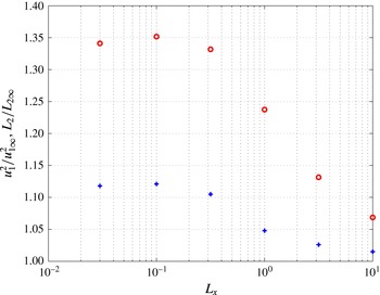
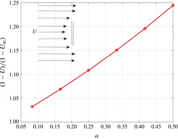
1 Introduction
Wind turbines and tidal-stream turbines most commonly have horizontal axis rotors (HAWTs and HATTs) and operate in highly turbulent flows, the atmospheric boundary layer (ABL) or its equivalent in tidal environments. The standard procedure for computing the resulting unsteady blade loading induced by incident turbulence is to assume the turbulence arriving at the rotor plane to be convected locally frozen by the mean flow up to the rotor plane as if the mean flow disturbance by the rotor were not present. The rotor blades are then assumed to react to this incident velocity distribution using some model (in a range of complexity from quasi-steady blade-element-momentum (BEM) to full unsteady computational fluid dynamics (CFD)) to obtain the blade response. Among the simplifications made, this approach does not account for the distortion of the incident turbulence itself by the mean strain field of the rotor as the turbulence approaches the rotor. Similarly, distortion of mean flow vorticity (in the ABL or tidal flow or wake profiles) incident on the rotor is not normally accounted for. In contrast the mean flow ‘blockage’ effect induced by the rotor’s own wake is taken into account in calculating the mean velocity field at the blades, as an essential part of that calculation.
Hunt (Reference Hunt1973) showed that the effect of distortion of incident turbulence can be substantial for a bluff body in turbulent flow and also that such flows often satisfy reasonably the requirements for linearised rapid distortion theory. These conditions are that the turbulence is weak and the mean strain field distorts the turbulence much more rapidly than the action of the turbulence on itself. The requirements are that
 $$\begin{eqnarray}\frac{u_{1}^{\prime }}{\overline{U}}\ll 1\end{eqnarray}$$
and
 $$\begin{eqnarray}\frac{u_{1}^{\prime }D}{\overline{U}L_{1\infty }}\ll 1,\end{eqnarray}$$
where
 $u_{1}^{\prime }$
is the root mean square (r.m.s.) streamwise velocity component of the turbulence,
 $\overline{U}$
is the mean flow velocity,
 $L_{1\infty }$
is the integral length scale of the turbulence and
 $D$
is a relevant length scale of the mean flow distortion, typically a body length scale. Applying this theory Hunt calculated the distortion of incident turbulence interacting with the upstream region of a circular cylinder.
Distortion of a turbulent velocity field arises from the stretching, tilting and displacement of the vorticity of the turbulence by the non-zero strain components of the mean flow field. If the length scale of the turbulent eddies is large compared with the length scale of the mean flow or body the distortion is small and may be neglected. But if the length scale ratio is not large the distortion can be considerable.
In the limit of a very small turbulence length scale the mean strain field and the relationship between vorticity and velocity can be treated as locally homogeneous and Batchelor & Proudman (Reference Batchelor and Proudman1954) (BP) developed a Lagrangian rapid distortion of turbulence (RDT) analysis to predict the intensity changes in a turbulent flow passing through a rapidly contracting duct such as a wind tunnel contraction. Condition (1.1) is reasonably satisfied in many turbulent flows including the contracting duct. Condition (1.2) is not usually satisfied since
 $L_{1\infty }$
is typically much smaller than the duct diameter, as noted in Batchelor & Proudman (Reference Batchelor and Proudman1954), unless either the turbulence is extremely weak,
 $u_{1}^{\prime }/\overline{U}\ll \ll 1$
or the streamwise mean velocity change in the contraction occurs over distance
 $D$
which is also much less than the duct diameter. This is not usually possible.
The mean flow generated by an actuator disc representing a turbine rotor extracting energy from a flow generates a mean flow field which is effectively the reverse of that in a contraction. The axial flow slows down and the streamlines diverge with the effect that the axial velocity component of the turbulence is amplified and the transverse velocity amplitudes are reduced. Modern wind and tidal turbines operate at high tip speed ratios and as a result are much more sensitive to changes in streamwise velocity than transverse velocity, increasingly so towards the blade tips. Hence this distortion amplification constitutes a potentially relevant issue. In addition, the divergence of the mean streamlines in the region of the rotor plane may be expected for the same reason to increase the transverse correlation length of the turbulence and hence the integrated unsteady forces on the rotor. For large industrial power-generating turbines in the ABL or tidal flows the turbulent eddy scales are typically similar to or significantly larger than the rotor diameter and the turbulence intensity is not extremely weak. Therefore the BP analysis is of limited value and the wavenumber analysis developed by Hunt (Reference Hunt1973) for length scale ratios of order 1 is more appropriate.
Hunt’s application of RDT developed the wavenumber analysis for turbulent flow around two-dimensional bluff bodies. In this method the distorted velocity field is computed from the distorted vorticity
 $\unicode[STIX]{x1D73B}$
of the turbulence by splitting the induced velocity into a rotational and an irrotational part:
 $\boldsymbol{u}=\boldsymbol{u}^{(I)}+\unicode[STIX]{x1D735}\unicode[STIX]{x1D719}$
, setting
 $\boldsymbol{u}^{(I)}=\unicode[STIX]{x1D735}\times \unicode[STIX]{x1D74D}$
with
 $\unicode[STIX]{x1D6FB}^{2}\unicode[STIX]{x1D74D}=-\unicode[STIX]{x1D73B}$
and
 $\unicode[STIX]{x1D719}$
to satisfy the boundary conditions with
 $\unicode[STIX]{x1D6FB}^{2}\unicode[STIX]{x1D719}=0$
. Goldstein (Reference Goldstein1978) followed the same approach for distortion of a turbulent flow around a two-dimensional bluff body (including compressibility of the flow) but derived a formulation allowing faster evaluation by setting the term
 $\boldsymbol{u}^{(I)}$
directly equal to the vortical part of the distorted turbulent velocity which is not associated with pressure fluctuations. This procedure avoids the lengthy evaluation of the three-component
 $\unicode[STIX]{x1D74D}$
vector, only requiring evaluation of the scalar
 $\unicode[STIX]{x1D719}$
. The necessary correction for solenoidal flow is incorporated into the irrotational term, thus for incompressible flows
 $\unicode[STIX]{x1D6FB}^{2}\unicode[STIX]{x1D719}=-\unicode[STIX]{x1D735}\boldsymbol{\cdot }\boldsymbol{u}^{(I)}$
. Goldstein & Durbin (Reference Goldstein and Durbin1980) used this method to study distortion of turbulence in a flow contracting into a two-dimensional intake. Majumdar & Peake (Reference Majumdar and Peake1998) extended the method to an axisymmetric contracting flow to analyse the effect of distortion of turbulence ingested by a multi-bladed fan rotor using asymptotic approximation in the small turbulence length scale, large blade number, high frequency, limits. Their objective was to compute the effect of distortion on the noise generated by interaction of the incident turbulence with the fan blades. In a low blade number case, Simonich et al. (Reference Simonich, Amiet, Schlinker and Greitzer1990) tracked elements of turbulent vorticity being distorted by the mean flow field of a helicopter rotor including both hover and forward flight cases, with a similar purpose of evaluating the blade noise generated due to inflow turbulence. Durbin (Reference Durbin1981) used RDT to study turbulence distortion by an axisymmetric body and also in his original thesis work Durbin (Reference Durbin1978) applied RDT to study the effect of mean shear on a turbulent flow. Hanazaki & Hunt (Reference Hanazaki and Hunt2004) included the effect of buoyancy body forces. These last two analyses are relevant to distortion of ABL turbulence but will not be considered in the present paper.
An alternative to this method of calculating the distorted turbulence velocity field is to compute it directly from the distorted vorticity field using the Biot–Savart integral solution of the Poisson equation relating them. This solution includes the irrotational part provided the flow boundary conditions are satisfied. It was used by Graham (Reference Graham1976) to compute distortion of turbulence incident on a two-dimensional porous plate under the condition of high porosity and therefore weak mean flow perturbation.
If a body surface is present its blockage effect on the turbulent flow must be included in any method of applying RDT. A surface panel method or for simple boundary geometries, vortex images may be used for this. RDT analysis usually neglects the effects of viscous dissipation of the turbulence. In many applications the Reynolds number is high enough for boundary layers on any body surfaces present in the flow to be thin relative to the length scale of the mean flow turbulence and no large-scale separations occur in the region being analysed. The influence of viscous effects is discussed in Hunt (Reference Hunt1973), Goldstein (Reference Goldstein1978) and Hunt (Reference Hunt1978). When these effects can be ignored the boundary condition to be satisfied at the body surface is that of zero normal flow. The effect of this is to induce a ‘blocking’ layer adjacent to the surface which was studied in detail using RDT theory by Hunt & Graham (Reference Hunt and Graham1978) for the special case of a plane surface in the absence of any mean velocity difference between the flow field and the body.
The aim of the present paper is to provide an assessment of the size of the turbulence distortion effect on the unsteady loading of HAWT and HATT rotors. The streamwise component of distorted turbulent velocity is computed at the rotor disc as this is the velocity component of incident turbulence to which the unsteady blade loading is most sensitive. For general length scale ratios following a wavenumber analysis requires a considerable multiplicity of numerical integrations incurring a correspondingly large computational effort. By selecting the disc centre as a representative point at which to compute the axial component of the distorted turbulent velocity and assuming the axisymmetric actuator disc model for the mean flow field of the rotor allows simplifications of axisymmetry to be used which considerably reduce the multiplicity of numerical integrations required. This is done in the present paper and estimates are then given for the variation of this distortion over the rest of the actuator disc.
In the case of a rotor flow not only is the incident vorticity of the turbulence distorted by the mean strain field of the rotor but the incident turbulent velocity field itself distorts the mean vorticity field of the rotor wake. This effect is not distortion of the incident turbulence but rather distortion (of the mean wake) by the incident turbulence. It is not usually considered in RDT analysis since a body wake, if present, is often somewhat removed from the flow region of interest. However, in the case of an open (i.e. non-ducted) turbine rotor the rotor wake has a large effect on the inflow at the rotor and the contribution of the turbulence in distorting the mean wake vorticity may be significant. The question of whether to include it in the assessment of distortion effects for turbulent flow incident on a rotor is discussed later.
Many numerical simulations of rotor blade forces due to incident turbulence have been published. The majority, e.g. Zahle & Sorensen (Reference Zahle and Sorensen2008), assume frozen turbulence incident on the rotor, but recently there have been computations which by modelling the vorticity as free vortex elements in the incident turbulent flow have taken account of the distortion of the incident turbulence, e.g. Branlard et al. (Reference Branlard, Papadakis, Gaunaa, Winckelmans and Larsen2015, Reference Branlard, Gaunaa, Mercier and Voutsinas2016).
Much of the actuator disc analysis for both the mean flow field and the distortion of incident turbulence through horizontal axis rotors has been developed for propeller or fan flows. In these cases the mean flow is accelerated by the power put into the flow by the actuator disc. In turbine applications where power is being extracted the same methods apply but nearly all the effects including distortion are reversed.
Experimental measurement of turbulence distortion due to the mean flow field of a rotor is difficult. Recent work by Hancock & Pascheke (Reference Hancock and Pascheke2014) has measured turbulence in the wake of a model wind turbine in a simulated turbulent atmospheric boundary layer with and without buoyancy forces present and distortion effects have been calculated from the BP analysis for the small length scale case (Farr & Hancock Reference Farr and Hancock2012).
Wind and tidal turbines usually operate in mean flows which are significantly sheared. With the increasing deployment of wind turbines in large wind farm arrays offshore the effect of wakes of upstream rotors incident on those further downstream has now become a significant issue in the prediction of performance and buffeting forces. These wakes generally meander (at low frequency, so may be considered here to be quasi-steady) under the effects of the largest turbulent eddies in the ABL and interaction with the sea surface (generally vortex image effects). They also contribute a considerable addition of their own turbulence to the ambient ABL turbulence. But the largest contribution both to the unsteady forces (Hankin & Graham Reference Hankin and Graham2012) and to the mean power (Argyle & Watson Reference Argyle and Watson2015) is usually from the mean wake deficit impacting a downstream turbine. The unsteady forces are generally largest when the wake is off the rotor axis overlapping the rotor about 50 % with its blades cutting the wake cyclically, and the power reduction is probably largest when wake and rotor overlap 100 %, i.e. they are coaxial. The incident flow fields therefore contain both mean and fluctuating vorticity and distortion may be an issue. Standard methods of computing the forces on the rotor blades assume that the mean flow, as for the turbulence, incident on each blade is that which would have been present in the incident flow field at the position in question in the absence of the rotor. Often simpler approximations based on conditions at hub height may be applied. As for incident turbulence the effect of the pressure field of the operating rotor is to cause distortion of the incident mean flow vorticity. This is simply a coupling between the incident mean vorticity and the mean pressure field of the rotor, quite distinct from any effects on the turbulence. The condition for the mean vorticity transport equation to be similarly linearised to evaluate this distortion is that the vorticity field is relatively weak. Thus
 $$\begin{eqnarray}|\unicode[STIX]{x1D735}\times \overline{U}|\frac{D}{\overline{U}}\ll 1.\end{eqnarray}$$
For the case of an incident wake generated by a rotor of the same size not too far upstream this leads to the requirement that
 $$\begin{eqnarray}\frac{\unicode[STIX]{x0394}\overline{U}}{\overline{U}}\ll 1,\end{eqnarray}$$
where
 $\unicode[STIX]{x0394}\overline{U}$
is a characteristic value of the wake mean velocity defect and the length scales of the wake and the downstream rotor will be similar.
If this is so the incident mean vorticity profile may be treated as a zero frequency component of turbulence with a deterministic distribution of the
 $\unicode[STIX]{x1D705}_{2},\unicode[STIX]{x1D705}_{3}$
wavenumbers and the linear RDT analysis followed. The simplest example which occurs when the incident wake is coaxial with the impacted rotor is calculated to demonstrate this.
The present paper is divided into sections. Section 2 presents the application of the locally homogeneous mean strain (BP) analysis to turbulent flow through an actuator disc. The theoretical analysis for the general length scale distortion case is given in § 3. This section includes the § 3.2 which gives the theoretical calculations of the actuator disc’s mean flow field. Section 4 discusses the effect of the turbulence on the mean wake vorticity and § 5 the application of the theory to incident mean wakes. The results and their asymptotic values are discussed in § 6 and the conclusions are summarised in § 7.
2 Small length scale limit
In this section theoretical predictions are derived for cases where the integral length scale of the turbulence
 $$\begin{eqnarray}L_{1\infty }=\int _{0}^{\infty }\frac{\overline{u_{1}(\boldsymbol{x})u_{1}(\boldsymbol{x}+x_{1}^{\prime }\unicode[STIX]{x1D73E})}\,\text{d}x_{1}^{\prime }}{\overline{u_{1}^{2}}(\boldsymbol{x})}\end{eqnarray}$$
is much smaller than the diameter of the actuator disc. Here and in the following
 $u_{1}$
is the streamwise component of the turbulent velocity
 $\boldsymbol{u}$
an overbar indicates a time average and
 $\unicode[STIX]{x1D73E}$
is the unit streamwise vector. In the following analyses the undisturbed incident turbulence will be assumed to be statistically homogeneous so that in (2.1)
 $L_{1\infty }$
is independent of
 $\boldsymbol{x}$
. This will not be true of the integral length scale or any other statistical quantity describing the turbulence in the distortion region, nor, of course, is it exactly true in the real cases of relevance.
2.1 One-dimensional mean flow turbine analysis
The coordinate directions in the streamwise and (any normal pair of) transverse directions are denoted by
 $x_{1}$
,
 $x_{2}$
,
 $x_{3}$
respectively. The corresponding mean flow velocity components are
 $(\overline{U}_{1},\overline{U}_{2},\overline{U}_{3})$
. The turbulent velocity components are
 $(u_{1},u_{2},u_{3})$
, with
 $(\unicode[STIX]{x1D705}_{1},\unicode[STIX]{x1D705}_{2},\unicode[STIX]{x1D705}_{3})$
the three components of the wavenumber vector
 $\unicode[STIX]{x1D73F}$
, in the corresponding directions. The suffix
 $\infty$
is used to indicate conditions sufficiently far upstream to be independent of the rotor and the suffix
 $0$
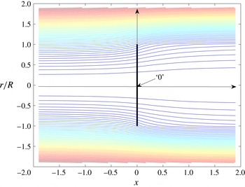
to indicate values at the rotor plane, usually at the origin which is at the centre of the rotor disc (figure 1).
The simplest model for the mean flow field of a HAWT (or HATT) rotor is the actuator disc model proposed by Froude (Reference Froude1911), Betz (Reference Betz1920) and Joukowsky (Reference Joukowsky1920). This replaces the disc swept by the rotor blades by a thin sheet of resistance to the flow. The model is the same as that proposed by Taylor (Reference Taylor1944) for a porous plate and indeed porous discs are often used as experimental analogues of rotors for wind tunnel testing of arrays. Within limits the mean flow field is represented quite well by this model but it omits the mean swirl in the wake.
From an axial momentum balance Betz (Reference Betz1920) showed that the rate of conversion of flow energy into mechanical energy is directly related to the induction of backflow by the rotor wake, which slows the mean flow into the rotor so that
 $\overline{U}_{1}(x_{1}=0)=(1-a)\overline{U}_{1\infty }$
where
 $a$
is the wake induction factor. In this simple model the rotor wake lies within a cylindrical sheet of vorticity and the induction factor and hence the mean streamwise velocity at the rotor plane are both constant over the disc. The strength of the vortex sheet is
 $2a\overline{U}_{1\infty }$
representing the helical vorticity shed from the rotor blade tips but omitting the small axial component which generates swirl. Far downstream the axial velocity within the wake is therefore
 $\overline{U}_{1w}=(1-2a)\overline{U}_{1\infty }$
and outside the wake it is
 $\overline{U}_{1\infty }$
.
Axial momentum analysis shows that this one-dimensional flow model predicts the power coefficient to be
 $$\begin{eqnarray}C_{P}=\frac{P}{\frac{1}{2}\unicode[STIX]{x1D70C}\overline{U}_{1\infty }^{3}A}=4a(1-a)^{2},\end{eqnarray}$$
where
 $P$
is the power extracted from the flow and
 $A(=\unicode[STIX]{x03C0}R^{2})$
is the swept area of the rotor disc.
This result leads to the well-known Betz limit that the maximum value possible for the power coefficient of an isolated open rotor is
 $16/27$
attained when
 $a=1/3$
. The result is sufficiently accurate for most real HAWTs and HATTs to be operated as close to this condition as possible to maximise efficiency. The model was later developed for propellers by Glauert (Reference Glauert1935) into the BEM method which forms the basis of industrial HAWT and HATT rotor design to the present day.
The actuator disc model of the mean flow field will be used in the present paper for the purpose of assessing distortion of turbulence incident on a rotor as it is the simplest model which is sufficiently realistic. This is so for high tip-speed-ratio rotors even if they have only two or three blades as is now the usual configuration of HAWTs and HATTs.
Similarly it will be assumed for the purposes of assessing the effect of distortion of incident turbulence that any turbulent flow of interest in the atmosphere or in a tidal channel can be represented by homogeneous isotropic turbulence convected by a uniform stream, conditions being based on those at the hub height of the rotor in the turbulent shear layer of the ABL or tidal flow. In what follows the mean free stream velocity will be taken as
 $(\overline{U}_{1\infty },\overline{U}_{2\infty },\overline{U}_{3\infty })=(1,0,0)$
so that all velocities are in effect non-dimensionalised by the free stream mean velocity and the radius of the actuator disc will similarly be taken to be
 $R=1$
so that all length scales are non-dimensionalised by the rotor radius.
The effect of the turbine on the turbulence when the turbulence length scale is much smaller than the rotor diameter:
 $L_{1\infty }\ll 1$
is examined first.
Mean flow streamlines through an actuator disc, induction factor
 $a=1/3$
.

Following the RDT analysis of BP for locally homogeneous strain the only information required is of the mean flow conditions at the position at which the distorted turbulent velocities are to be calculated relative to the upstream conditions. In the present work the distorted velocity field is to be calculated at the rotor plane in order to assess the effect of distortion on what would normally be assumed to be frozen incident turbulence impacting the rotor. Therefore the blocking effect of the blade surfaces should not be included in the distortion calculation. The issue of rotor mean wake distortion by the turbulent velocities is considered later but has no effect at the rotor plane in the limit of very small turbulence length scale. Since the buffet forces on rotor blades operating at high tip speed ratio (as is usual) are mainly sensitive to the axial
 $u_{1}$
component of the turbulence, therefore in this paper this velocity component will be calculated. If the disc centre ((0, 0, 0) in figure 1) is taken as a representative point the simplifications of axisymmetry and plane strain can be used which reduce the computational effort very considerably. But off the axis elements of the turbulence vorticity are subject to rotation (tilting) in addition to the stretching or compression by the pure strain
 $(\unicode[STIX]{x2202}\overline{U_{i}}/\unicode[STIX]{x2202}x_{i})~i=1,2$
or 3. Durbin (Reference Durbin1981) has derived this contribution for the small length scale case of turbulence incident on an axisymmetric body. His approach will be followed here for points off the axis.
2.2 Distortion of small length scale turbulence
The distorted streamwise turbulent velocity
 $u_{1}$
at the centre of the disc (0,0,0) is first considered. The mean flow axial velocity at (0,0,0) is
 $$\begin{eqnarray}\overline{U}_{1}(0)=1-a\end{eqnarray}$$
which corresponds to a mean flow expansion.
The actuator disc flow field close to the axis is the opposite of that for a wind tunnel contraction and is similarly a pure strain. The BP analysis as given in Batchelor (Reference Batchelor1953) develops the rapid distortion analysis for this case in terms of the mean flow contraction coefficient
 $c$
 $(=\overline{U}_{1}(final)/\overline{U}_{1\infty }(initial))>1$
. For the actuator disc case the equivalent ‘contraction’ coefficient
 $c<1$
. Writing
 $\unicode[STIX]{x1D73B}(\boldsymbol{x})=\unicode[STIX]{x1D735}\times \boldsymbol{u}(\boldsymbol{x})$
as the vorticity of the turbulent fluctuations at a general point
 $\boldsymbol{x}$
with corresponding value far upstream
 $\unicode[STIX]{x1D73B}_{\infty }(\unicode[STIX]{x1D743}_{\infty })$
then the Lagrangian specification of the motion used by Batchelor shows that in the absence of viscous forces
 $$\begin{eqnarray}\unicode[STIX]{x1D701}_{i}(\boldsymbol{x})=\frac{\unicode[STIX]{x2202}x_{i}}{\unicode[STIX]{x2202}\unicode[STIX]{x1D709}_{j\infty }}\unicode[STIX]{x1D701}_{j\infty }(\unicode[STIX]{x1D743}_{\infty }),\end{eqnarray}$$
where
 $\boldsymbol{x}$
is the coordinate of a fluid particle originally upstream with Lagrangian coordinate
 $\unicode[STIX]{x1D743}_{\infty }$
on the same streamline. Thus the vorticity is intensified or diminished and distributed between components according to the strain tensor
 $(\unicode[STIX]{x2202}x_{i}/\unicode[STIX]{x2202}\unicode[STIX]{x1D709}_{j\infty })$
.
The turbulent velocity field expressed in wavenumber form
 $$\begin{eqnarray}\boldsymbol{u}(\boldsymbol{x})=\int _{-\infty }^{\infty }\int _{-\infty }^{\infty }\int _{-\infty }^{\infty }\hat{\boldsymbol{u}}(\unicode[STIX]{x1D73F})\text{e}^{\text{i}(\unicode[STIX]{x1D714}t-\unicode[STIX]{x1D73F}\boldsymbol{x})}\,\text{d}\unicode[STIX]{x1D73F}\end{eqnarray}$$
where
 $Gk\unicode[STIX]{x1D714}$
is angular frequency, can be calculated from the vorticity field through the relationship
 $$\begin{eqnarray}\unicode[STIX]{x1D6FB}^{2}\boldsymbol{u}=-\unicode[STIX]{x1D735}\times \unicode[STIX]{x1D73B}(\boldsymbol{x}).\end{eqnarray}$$
If the strain tensor may be considered to vary very little over the length scale of the turbulence, which is the strain homogeneity assumption for small length scale turbulence, then (2.6) may be solved locally with the strain tensor terms as constants rather than solving over the whole strain field. Therefore in wavenumber form the velocity at the disc can be expressed in terms of a distorted wavenumber
 $\unicode[STIX]{x1D74C}$
by
 $$\begin{eqnarray}\unicode[STIX]{x1D712}^{2}\hat{u} _{i}(\unicode[STIX]{x1D74C})=-\unicode[STIX]{x1D750}_{ijm}\unicode[STIX]{x1D716}_{npq}\frac{\unicode[STIX]{x2202}x_{m}}{\unicode[STIX]{x2202}\unicode[STIX]{x1D709}_{n\infty }}\frac{\unicode[STIX]{x2202}\unicode[STIX]{x1D709}_{m\infty }}{\unicode[STIX]{x2202}x_{j}}\unicode[STIX]{x1D705}_{p}\unicode[STIX]{x1D705}_{m}\hat{u} _{q\infty }(\unicode[STIX]{x1D73F}),\end{eqnarray}$$
where the distorted wavenumber
 $\unicode[STIX]{x1D74C}$
is related to the undistorted wavenumbers
 $\unicode[STIX]{x1D73F}$
by
 $$\begin{eqnarray}\unicode[STIX]{x1D712}_{i}=\frac{\unicode[STIX]{x2202}\unicode[STIX]{x1D709}_{j\infty }}{\unicode[STIX]{x2202}x_{i}}\unicode[STIX]{x1D705}_{j}\end{eqnarray}$$
and
 $\unicode[STIX]{x1D750}_{ijm}$
is the unit alternating tensor. In the case of pure strain as for a wind tunnel contraction or for the rotor flow near the axis only the diagonal terms of the strain tensor,
 $(\unicode[STIX]{x2202}x_{1}/\unicode[STIX]{x2202}\unicode[STIX]{x1D709}_{1\infty })=c,(\unicode[STIX]{x2202}x_{2}/\unicode[STIX]{x2202}\unicode[STIX]{x1D709}_{2\infty })=(\unicode[STIX]{x2202}x_{3}/\unicode[STIX]{x2202}\unicode[STIX]{x1D709}_{3\infty })=1/\sqrt{c}$
, are non-zero. The relationship between the spectral tensors
 $\unicode[STIX]{x1D731}_{11}$
of the distorted and undistorted turbulence, time mean products of the wavenumber amplitudes
 $\hat{u} _{1}$
with their complex conjugates, then simplifies greatly to
 $$\begin{eqnarray}\unicode[STIX]{x1D731}_{11}(\unicode[STIX]{x1D705})=\frac{\unicode[STIX]{x1D705}^{4}}{\unicode[STIX]{x1D705}_{\infty }^{4}}\unicode[STIX]{x1D731}_{11\infty }(\unicode[STIX]{x1D705}_{\infty }).\end{eqnarray}$$
The spectrum tensor for the undistorted upstream streamwise turbulence velocity, assumed isotropic and homogeneous, has the form (Batchelor Reference Batchelor1953)
 $$\begin{eqnarray}\unicode[STIX]{x1D731}_{11\infty }=E(\unicode[STIX]{x1D705})\frac{\unicode[STIX]{x1D70F}^{2}}{4\unicode[STIX]{x03C0}\unicode[STIX]{x1D705}^{4}},\end{eqnarray}$$
where
 $\unicode[STIX]{x1D70F}^{2}=\unicode[STIX]{x1D705}_{2}^{2}+\unicode[STIX]{x1D705}_{3}^{2}$
and
 $E(\unicode[STIX]{x1D705})$
is the turbulence energy spectrum function. Therefore, its
 $(\unicode[STIX]{x1D705}_{1})$
frequency spectrum is
 $$\begin{eqnarray}\unicode[STIX]{x1D719}_{11\infty }(\unicode[STIX]{x1D705}_{1})=\int _{-\infty }^{\infty }\int _{-\infty }^{\infty }E(\unicode[STIX]{x1D705})\frac{\unicode[STIX]{x1D70F}^{2}\,\text{d}\unicode[STIX]{x1D705}_{2}\,\text{d}\unicode[STIX]{x1D705}_{3}}{4\unicode[STIX]{x03C0}\unicode[STIX]{x1D705}^{4}}\end{eqnarray}$$
and the frequency spectrum for the distorted streamwise turbulence velocity at the disc in the region of the axis becomes
 $$\begin{eqnarray}\unicode[STIX]{x1D719}_{11}(\unicode[STIX]{x1D705}_{1})=\int _{-\infty }^{\infty }\int _{-\infty }^{\infty }E(\unicode[STIX]{x1D705})\frac{\unicode[STIX]{x1D70F}^{2}\,\text{d}\unicode[STIX]{x1D705}_{2}\,\text{d}\unicode[STIX]{x1D705}_{3}}{4\unicode[STIX]{x03C0}(c^{-2}\unicode[STIX]{x1D705}_{1}^{2}+c^{2}\unicode[STIX]{x1D70F}^{2})^{2}}.\end{eqnarray}$$
Integrating these two spectra with respect to
 $\unicode[STIX]{x1D705}_{1}$
, substituting
 $\unicode[STIX]{x1D705}_{1}=\unicode[STIX]{x1D705}\cos \unicode[STIX]{x1D703}$
and
 $\unicode[STIX]{x1D70F}=\unicode[STIX]{x1D705}\sin \unicode[STIX]{x1D703}$
, the ratio of the mean square of the streamwise turbulence velocity at the disc centre to its upstream value is
 $$\begin{eqnarray}\displaystyle \unicode[STIX]{x1D707}(c) & = & \displaystyle \frac{\overline{u_{1}^{2}}}{\overline{u_{1\infty }^{2}}}=\frac{\displaystyle \int _{-\infty }^{\infty }\int _{-\infty }^{\infty }\int _{-\infty }^{\infty }E(\unicode[STIX]{x1D705})\frac{\unicode[STIX]{x1D70F}^{2}\,\text{d}\unicode[STIX]{x1D705}_{1}\,\text{d}\unicode[STIX]{x1D705}_{2}\,\text{d}\unicode[STIX]{x1D705}_{3}}{4\unicode[STIX]{x03C0}(c^{-2}\unicode[STIX]{x1D705}_{1}^{2}+c^{2}\unicode[STIX]{x1D70F}^{2})^{2}}}{\displaystyle \int _{-\infty }^{\infty }\int _{-\infty }^{\infty }\int _{-\infty }^{\infty }E(\unicode[STIX]{x1D705})\frac{\unicode[STIX]{x1D70F}^{2}\,\text{d}\unicode[STIX]{x1D705}_{1}\,\text{d}\unicode[STIX]{x1D705}_{2}\,\text{d}\unicode[STIX]{x1D705}_{3}}{4\unicode[STIX]{x03C0}\unicode[STIX]{x1D705}^{4}}}\nonumber\\ \displaystyle & = & \displaystyle \frac{\displaystyle \int _{0}^{\unicode[STIX]{x03C0}}\frac{\sin ^{3}\unicode[STIX]{x1D703}\,\text{d}\unicode[STIX]{x1D703}}{(c^{-2}\cos ^{2}\unicode[STIX]{x1D703}+c\sin ^{2}\unicode[STIX]{x1D703})^{2}}}{\displaystyle \int _{0}^{\unicode[STIX]{x03C0}}\sin ^{3}\unicode[STIX]{x1D703}\,\text{d}\unicode[STIX]{x1D703}}\nonumber\\ \displaystyle & = & \displaystyle \frac{3(\sqrt{s}+(s-1)\tan ^{-1}(\sqrt{s}))}{4c^{2}s^{3/2}},\end{eqnarray}$$
where
 $s=c^{-3}-1$
. This result, which may be obtained directly from the BP result setting
 $c<1$
and taking account of the imaginary square root, was given by Farr & Hancock (Reference Farr and Hancock2012). It is close to but just less than the upper limit of the amplification ratio of intensity due to distortion over all length scales. It is independent of the form of the turbulence energy spectrum function
 $E(\unicode[STIX]{x1D705})$
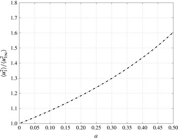
which divides out in taking the ratio. Figure 2 shows a plot of this ratio versus the induction factor
 $a=(1-c)$
. In this case,
 $L_{1\infty }\rightarrow 0$
, the distortion of the streamwise turbulence intensity
 $\overline{u_{1}^{2}}/\overline{u^{2}}_{1\infty }=1.341$
when
 $a=1/3$
. For
 $a>1/2$
actuator disc theory predicts mean flow reversal in the wake and although wake reversal does occur in reality, the model breaks down.
Mean square turbulence intensity ratio
 $\overline{u_{1}^{2}}/\overline{u_{1\infty }^{2}}$
versus induction factor
 $a$
for
 $L_{1\infty }\rightarrow 0$
.

In order to calculate the spectrum
 $\unicode[STIX]{x1D719}_{11}$
of the distorted turbulence it is necessary to specify the form of the energy spectrum function
 $E(\unicode[STIX]{x1D705})$
. The turbulence of the wind in a neutral ABL is usually represented by an empirical spectrum such as the von Kármán spectrum (Deaves & Harris Reference Deaves and Harris1978) that incorporates a
 $-5/3$
exponent at high frequencies. This distribution is also considered to be representative of moderately homogeneous turbulence in a wide range of flows, including grid-generated turbulence relevant to some wind tunnel tests of turbulence effects on model rotors, turbulence in tidal streams and possibly wake-induced turbulence within large wind farm arrays. The von Kármán spectrum will be assumed in the present paper to represent the turbulence adequately. Mann (Reference Mann1994) discusses other forms of spectra taking into account the anisotropy of the ABL and the ground plane blockage. It is unlikely that the results obtained here using the von Kármán distribution would change greatly if alternatives such as these, for example, the frequently used Kaimal spectrum (Kaimal et al.
Reference Kaimal, Izumi, Wyngaard and Cote1972) were used instead.
The von Kármán spectrum representing homogeneous, isotropic turbulence with a substantial inertial subrange, is described by the triple wavenumber energy spectrum function:
 $$\begin{eqnarray}E(\unicode[STIX]{x1D705})=\frac{C\overline{u^{2}}_{1\infty }\unicode[STIX]{x1D705}^{\ast 4}}{(1+\unicode[STIX]{x1D705}^{\ast 2})^{17/6}},\end{eqnarray}$$
where
 $$\begin{eqnarray}\unicode[STIX]{x1D73F}^{\ast }=g_{0}L_{1\infty }\unicode[STIX]{x1D73F},\end{eqnarray}$$
 $g_{0}$
is a ratio of Gamma functions
 $$\begin{eqnarray}g_{0}=\frac{\unicode[STIX]{x1D6E4}\left(\frac{1}{3}\right)}{\unicode[STIX]{x1D6E4}\left(\frac{1}{2}\right)\unicode[STIX]{x1D6E4}\left(\frac{5}{6}\right)}=1.339\end{eqnarray}$$
and the constant
 $C=(220/9)L_{1\infty }$
.
Hence the triple wavenumber spectrum function of the turbulence is
 $$\begin{eqnarray}\unicode[STIX]{x1D731}_{ij}(\unicode[STIX]{x1D705}_{1}^{\ast },\unicode[STIX]{x1D705}_{2}^{\ast },\unicode[STIX]{x1D705}_{3}^{\ast })=\frac{C(g_{0}L_{1\infty })^{2}\overline{u^{2}}_{1\infty }\unicode[STIX]{x1D705}^{\ast 2}}{4\unicode[STIX]{x03C0}(1+\unicode[STIX]{x1D705}^{\ast 2})^{17/6}}\left\{\unicode[STIX]{x1D6FF}_{ij}-\frac{\unicode[STIX]{x1D705}_{i}^{\ast }\unicode[STIX]{x1D705}_{j}^{\ast }}{\unicode[STIX]{x1D705}^{\ast 2}}\right\}.\end{eqnarray}$$
For spectra involving cross-stream components a simple method to accommodate some effects of anisotropy in ABL turbulence is to replace
 $\overline{u^{2}}_{1\infty }$
in (2.17) by the relevant turbulence intensity. But for the streamwise component
 $i=j=1$
:
 $$\begin{eqnarray}\unicode[STIX]{x1D731}_{11}(\unicode[STIX]{x1D705}_{1}^{\ast },\unicode[STIX]{x1D705}_{2}^{\ast },\unicode[STIX]{x1D705}_{3}^{\ast })=\frac{C(g_{0}L_{1\infty })^{2}\overline{u^{2}}_{1\infty }\unicode[STIX]{x1D70F}^{\ast 2}}{4\unicode[STIX]{x03C0}(1+\unicode[STIX]{x1D705}^{\ast 2})^{17/6}}.\end{eqnarray}$$
This triple wavenumber spectrum tensor is integrated with respect to the radial wavenumber
 $\unicode[STIX]{x1D70F}$
to give the one-dimensional frequency spectrum:
 $$\begin{eqnarray}\unicode[STIX]{x1D719}_{11}(\unicode[STIX]{x1D705}_{1}^{\ast })=\int _{0}^{\infty }\frac{\unicode[STIX]{x1D705}^{\ast 4}\unicode[STIX]{x1D70F}^{\ast 3}\,\text{d}\unicode[STIX]{x1D70F}^{\ast }}{2(c^{-2}\unicode[STIX]{x1D705}_{1}^{\ast 2}+c\unicode[STIX]{x1D70F}^{\ast 2})^{2}(1+\unicode[STIX]{x1D705}_{1}^{\ast 2}+\unicode[STIX]{x1D70F}^{\ast 2})^{17/6}}.\end{eqnarray}$$
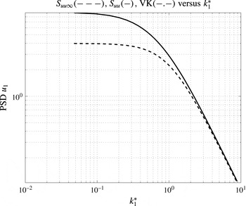
The above integral has been evaluated numerically and the resulting power spectral density (PSD) of the
 $\unicode[STIX]{x1D705}_{1}$
spectrum for the distorted turbulence in the optimum operating case,
 $a=1/3$
, i.e.
 $c=2/3$
is compared with the undistorted upstream turbulence spectrum
 $\unicode[STIX]{x1D719}_{11\infty }$
in figure 3.
The amplification ratio for large values of
 $\unicode[STIX]{x1D705}_{1}^{\ast }\rightarrow \infty$
in the small length scale limit is
 $$\begin{eqnarray}\displaystyle \frac{\unicode[STIX]{x1D719}_{11}}{\unicode[STIX]{x1D719}_{11\infty }}(\unicode[STIX]{x1D705}_{1}\rightarrow \infty ) & = & \displaystyle \frac{55\displaystyle \int _{0}^{\infty }\frac{\unicode[STIX]{x1D70F}^{\ast 3}\,\text{d}\unicode[STIX]{x1D70F}^{\ast }}{(c^{-2}\unicode[STIX]{x1D705}_{1}^{\ast 2}+c\unicode[STIX]{x1D70F}^{\ast 2})^{2}(\unicode[STIX]{x1D705}_{1}^{\ast 2}+\unicode[STIX]{x1D70F}^{\ast 2})^{5/6}}}{18\unicode[STIX]{x1D705}_{1}^{\ast -5/3}}\nonumber\\ \displaystyle & = & \displaystyle c^{4}._{2}F_{1}(2,2;17/6;1-c^{3}),\end{eqnarray}$$
where from Gradshteyn & Ryzhik (Reference Gradshteyn and Ryzhik1980), integral result 3.197,
 $_{2}F_{1}$
is the Hypergeometric function.
Therefore
 $(\unicode[STIX]{x1D719}_{11}/\unicode[STIX]{x1D719}_{11\infty })(\unicode[STIX]{x1D705}_{1}\rightarrow \infty )=1.033$
when
 $a=1/3$
. The ratio of the zero frequency intercept value of the spectrum can be obtained by using (2.19) and substituting
 $\unicode[STIX]{x1D705}_{1}^{\ast }=0$
. The expression for this ratio then simplifies to
 $c^{-2}$
with value
 $=2.25$
when
 $a=1/3$
. Both these asymptotic ratios are consistent with the spectra shown in figure 3.
Frequency spectrum
 $\unicode[STIX]{x1D719}_{11}$
for induction factor
 $a=1/3$
; solid line distorted, dashed line undistorted.

2.3 Transverse length scale of the distorted turbulence
In this case the magnitudes of the length scales of the turbulence at the rotor change due to distortion by the mean strain field. In a propeller or fan flow field
 $c>1$
causes extension of
 $L_{1}$
and contraction of
 $L_{2}$
(Majumdar & Peake Reference Majumdar and Peake1998) whereas in a turbine flow,
 $c<1$
, the opposite is the case and the transverse integral length scale
 $L_{2}$
is increased by the distortion. This potentially increases the correlation of the unsteady forces on the rotor blades and hence the r.m.s. of the integrated unsteady axial force on the rotor as a whole. The transverse length scale
 $L_{2}$
of the turbulence after distortion is
 $$\begin{eqnarray}\displaystyle L_{2} & = & \displaystyle \frac{\displaystyle \int _{0}^{\infty }\overline{u_{1}(0)u_{1}(y)}\,\text{d}y}{\overline{u_{1}^{2}(0)}}\nonumber\\ \displaystyle & = & \displaystyle \frac{1}{\overline{u_{1}^{2}}(0)}\int _{0}^{\infty }\int _{-\infty }^{\infty }\int _{-\infty }^{\infty }\int _{-\infty }^{\infty }E(\unicode[STIX]{x1D705})\frac{\unicode[STIX]{x1D70F}^{2}\,\text{d}\unicode[STIX]{x1D705}_{1}\,\text{d}\unicode[STIX]{x1D705}_{2}\,\text{d}\unicode[STIX]{x1D705}_{3}}{4\unicode[STIX]{x03C0}(c^{-2}\unicode[STIX]{x1D705}_{1}^{2}+c\unicode[STIX]{x1D70F}^{2})^{2}}\text{e}^{\text{i}\unicode[STIX]{x1D705}_{2}y^{\prime }}\,\text{d}y\end{eqnarray}$$
since the distortion factor in the integral is homogeneous, independent of
 $y$
in the limit
 $L_{1\infty }\rightarrow 0$
where
 $y^{\prime }=c^{-1/2}y$
due to the transverse displacement of the streamlines of the mean flow.
Simplifying by carrying out the integrations with respect to
 $y$
and
 $\unicode[STIX]{x1D705}_{2}$
and substituting the integral expression for
 $\overline{u_{1}^{2}}(0)$
leads to
 $$\begin{eqnarray}\frac{L_{2}}{L_{1\infty }}=\frac{g_{0}\displaystyle \int _{0}^{\unicode[STIX]{x03C0}}\frac{\sin ^{2}\unicode[STIX]{x1D703}\,\text{d}\unicode[STIX]{x1D703}}{(c^{-2}\cos ^{2}\unicode[STIX]{x1D703}+c\sin ^{2}\unicode[STIX]{x1D703})^{2}}\int _{0}^{\infty }\frac{E(\unicode[STIX]{x1D705}^{\ast })\,\text{d}\unicode[STIX]{x1D705}^{\ast }}{\unicode[STIX]{x1D705}^{\ast }}}{c^{1/2}\displaystyle \int _{0}^{\unicode[STIX]{x03C0}}\frac{\sin ^{3}\unicode[STIX]{x1D703}\,\text{d}\unicode[STIX]{x1D703}}{(c^{-2}\cos ^{2}\unicode[STIX]{x1D703}+c\sin ^{2}\unicode[STIX]{x1D703})^{2}}\int _{0}^{\infty }E(\unicode[STIX]{x1D705}^{\ast })\,\text{d}\unicode[STIX]{x1D705}^{\ast }}.\end{eqnarray}$$
In this case the result depends on the form of
 $E(\unicode[STIX]{x1D705})$
since the integrals involving the turbulence energy can no longer be divided out.
Assuming the von Kármán form for
 $E(\unicode[STIX]{x1D705})$
as before, the integrals for the transverse length scale ratio can be evaluated to give
 $$\begin{eqnarray}\frac{L_{2}}{L_{2\infty }}=\frac{4cs^{3/2}}{3(\sqrt{s}+(s-1)\tan ^{-1}(\sqrt{s}))},\end{eqnarray}$$
with
 $s=c^{-3}-1$
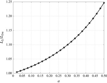
. The transverse length scale amplification ratio
 $L_{2}/L_{2\infty }$
is plotted against the induction factor
 $a$
in figure 4. This ratio is smaller than
 $c^{-1/2}$
the transverse divergence ratio of the mean streamlines. When
 $a=1/3$
the amplification factor for the transverse length scale ratio is 1.118.
For small length scales the integrated fluctuating force induced on the rotor will be approximately proportional to the fluctuating axial velocity multiplied by the correlation area. The effect of distortion of the incident turbulence on this integrated buffeting force induced by the turbulence on the rotor as a whole is significant, amplifying the r.m.s. axial rotor force amplitude by a factor of approximately
 $$\begin{eqnarray}\frac{L_{2}^{2}}{L_{2\infty }^{2}}\sqrt{\frac{\overline{u^{2}}_{1}}{\overline{u^{2}}_{1\infty }}}=1.45.\end{eqnarray}$$
Transverse length scale amplification ratio
 $(L_{2}/L_{2\infty })$
versus induction factor
 $a$
,
 $L_{1\infty }\rightarrow 0$
.

2.4 Distorted turbulence intensity off the axis
Durbin (Reference Durbin1981) has developed the small length scale analysis for distortion at general points in the flow field of an axisymmetric obstacle. As for the BP analysis, the strain field is assumed to be slowly varying so that the strain terms can be treated locally as constants simplifying the calculation of the distorted turbulent velocity from the distorted vorticity. The strain tensor
 $\unicode[STIX]{x2202}x_{i}/\unicode[STIX]{x2202}x_{j\infty }$
in this general case contains non-zero off-diagonal terms
 $(i\neq j)$
which represent tilting and bending of vortex lines in the
 $(r,x_{1})$
plane. Since the mean axial velocity
 $\overline{U}_{1}=(1-a)$
is constant over the actuator disc the pure strain terms on the diagonal of the strain tensor are unchanged. The result of this is that the distorted turbulent velocity vector is equal to the value resulting from pure strain alone multiplied by a rotation matrix leading to (Durbin Reference Durbin1981, equation (23))
 $$\begin{eqnarray}\frac{\overline{u_{1}^{2}}}{\overline{u_{1\infty }^{2}}}=\cos ^{2}(\unicode[STIX]{x1D6FD}+\unicode[STIX]{x1D6FF})\unicode[STIX]{x1D707}(c)+\sin ^{2}(\unicode[STIX]{x1D6FD}+\unicode[STIX]{x1D6FF})\unicode[STIX]{x1D708}(c),\end{eqnarray}$$
where
 $\unicode[STIX]{x1D707}(c)$
and
 $\unicode[STIX]{x1D708}(c)$
are the distortion factors given in Batchelor (Reference Batchelor1953) for in-line and transverse mean square turbulence velocities.
 $\unicode[STIX]{x1D707}(c)$
for
 $c<1$
is given in (2.13). Similarly
 $\unicode[STIX]{x1D708}(c)$
taking account of the imaginary square root when
 $c<1$
, is
 $$\begin{eqnarray}\unicode[STIX]{x1D708}(c)=\frac{3}{4}\left(c-\frac{1}{2c^{2}s^{3/2}}[\sqrt{s}-(s+1)\tan ^{-1}\sqrt{s}]\right),\end{eqnarray}$$
where
 $s=c^{-3}-1$
. In (2.25)
 $\unicode[STIX]{x1D6FD}$
is the rotation angle due to the gradient across the mean flow streamlines of the drift function
 $\unicode[STIX]{x0394}x_{1}(x_{1},r)$
. This is the
 $x_{1}$
-displacement of a fluid particle convected by the non-uniform mean flow field relative to the position it would have reached at the same time in uniform flow
 $\overline{\boldsymbol{U}_{\infty }}(=(1,0,0))$
and is given explicitly in (3.23).
 $\unicode[STIX]{x1D6FF}=\tan ^{-1}((\sqrt{\overline{U}_{2}^{2}+\overline{U}_{3}^{2}})/\overline{U}_{1})$
is the rotation angle due to the inclination of the mean flow streamlines. For the actuator disc mean flow field, except close to the tip region
 $(r=1,x_{1}=0)$
, these two rotation angles are in opposite directions, are of comparable size and are small so that the combined rotation angle
 $(\unicode[STIX]{x1D6FD}+\unicode[STIX]{x1D6FF})$
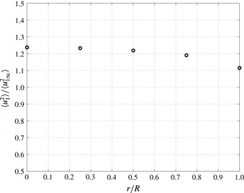
is small. Evaluating the right-hand side of (2.25) the ratio
 $\overline{u_{1}^{2}}/\overline{u_{1\infty }^{2}}$
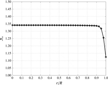
falls gradually with radial distance from the axis and rapidly at the tip as shown in figure 5 for the case when
 $a=1/3$
.
The radial component of the mean velocity given by actuator disc theory is logarithmically singular at the rotor tip. Therefore the rotation angle
 $\unicode[STIX]{x1D6FF}$
based on this mean flow field takes the value
 $\unicode[STIX]{x03C0}/2$
there. The angle
 $\unicode[STIX]{x1D6FD}$
is finite at the tip but discontinuous between
 $r<1$
and
 $r>1$
. The actuator disc flow field has been retained for the present calculations but being unrepresentative in the tip region a tip correction factor is normally applied in BEM theory to cause the blade loading to approach zero appropriately at the tip.
Radial variation of distorted streamwise intensity for zero length scale and
 $a=1/3$
.

3 Distortion of general length scale turbulence
Accurate estimation of the turbulence integral length scale in the bottom layer of the ABL is difficult. Since sufficiently long time histories of statistically constant data may not be available the low frequency end of the spectrum is very ‘jagged’ and estimates from the ‘knee’ of the spectrum where
 $k_{1}\unicode[STIX]{x1D719}_{11}(k_{1})$
is maximum may be better (Mann Reference Mann1994). In addition the turbulence of relevance to typical HAWTs is subject to some ground-plane blockage effects (Hunt & Graham Reference Hunt and Graham1978; Mann Reference Mann1994). Values of the integral length scale,
 $L_{1\infty }$
, depend on how it is estimated, at what height above the ground and in the ABL conditions. For heights in the region of 50 m to 100 m estimates vary between approximately 50 m and 250 m (Teunissen Reference Teunissen1970; Irwin Reference Irwin1977; Deaves & Harris Reference Deaves and Harris1978; Mann Reference Mann1994). Rotor diameters of most power-generating wind turbines currently being deployed are larger than 100 m and heading towards 200 m. Tidal-stream turbines are still at the stage of prototype testing. Many are likely to operate in shallow tidal channels with rotor diameters (
 $O$
(20 m)) equal to approximately half of the channel depth. In these cases also, depending on the channel-bed conditions, the turbulence length scale is likely to be of the same order of magnitude as the rotor diameter, e.g. Milne et al. (Reference Milne, Day, Sharma and Flay2016). Therefore in assessing the influence of turbulence distortion on rotor blade loading, distortion analysis for length scale ratios
 $O$
(1) must be carried out, rather than using the results for
 $L_{1\infty }\rightarrow 0$
. Exceptions to this where the small length scale ratio case may be more relevant occur in some model rotor tests in simulated ABL or other turbulence in wind tunnels and perhaps for well mixed wake-generated turbulence deep within wind farm or tidal farm arrays. But in individual wake impact cases the impact on the downstream turbine blades cutting through an off-axis mean wake velocity defect is often much larger than any effect of the wake turbulence, e.g. Hankin & Graham (Reference Hankin and Graham2012). Where details of rotor loading are to be measured in wind tunnel tests model rotors cannot be made too small for practical reasons, not least to retain reasonable aerodynamic characteristics for the blades. It is often difficult to generate large length scale turbulence in a wind tunnel and as a result the turbulence length scale to rotor diameter ratio may be smaller than is representative of the ratio at full scale. In such cases the small length scale ratio limit may give useful information about possible unrepresentative distortion effects.
3.1 Vorticity transport by the mean flow field of an actuator disc
The general case of arbitrary turbulence length scale to rotor radius ratio will now be considered. The vorticity transport equation for unsteady incompressible flow normalised on the mean free stream velocity as before, is
 $$\begin{eqnarray}\frac{\unicode[STIX]{x2202}Z_{i}}{\unicode[STIX]{x2202}t}+U_{j}\frac{\unicode[STIX]{x2202}Z_{i}}{\unicode[STIX]{x2202}x_{j}}=Z_{j}\frac{\unicode[STIX]{x2202}U_{i}}{\unicode[STIX]{x2202}x_{j}}+Re^{-1}\frac{\unicode[STIX]{x2202}^{2}Z_{i}}{\unicode[STIX]{x2202}x_{j}\unicode[STIX]{x2202}x_{j}},\end{eqnarray}$$
where
 $\boldsymbol{Z}=\unicode[STIX]{x1D735}\times \boldsymbol{U}$
is the vorticity of the flow and
 $Re=UR/\unicode[STIX]{x1D708}$
is the mean flow Reynolds number.
Splitting the velocity and other flow variables into mean and fluctuating parts:
 $$\begin{eqnarray}\displaystyle & \displaystyle U_{i}(x_{j},t)=\overline{U}_{i}(x_{j})+u_{i}(x_{j},t) & \displaystyle\end{eqnarray}$$
 $$\begin{eqnarray}\displaystyle & \displaystyle \rightarrow \unicode[STIX]{x1D6FF}_{i,1}+u_{i\infty }(x_{j},t)\quad x_{1}\rightarrow -\infty & \displaystyle\end{eqnarray}$$
and
 $$\begin{eqnarray}\displaystyle & \displaystyle Z_{i}(x_{j},t)=\overline{\unicode[STIX]{x1D701}}_{i}(x_{j})+\unicode[STIX]{x1D701}_{i}(x_{j},t) & \displaystyle\end{eqnarray}$$
 $$\begin{eqnarray}\displaystyle & \displaystyle \rightarrow \unicode[STIX]{x1D701}_{i\infty }(x_{j},t)\quad x_{1}\rightarrow -\infty . & \displaystyle\end{eqnarray}$$
The flow is assumed to satisfy the requirements for RDT that in terms of the non-dimensionalised quantities
 $$\begin{eqnarray}\displaystyle & \displaystyle \sqrt{\overline{u^{2}}_{1\infty }}\ll 1 & \displaystyle\end{eqnarray}$$
 $$\begin{eqnarray}\displaystyle & \displaystyle \frac{\sqrt{\overline{u^{2}}_{1\infty }}}{L_{1\infty }}\ll 1 & \displaystyle\end{eqnarray}$$
 $$\begin{eqnarray}\displaystyle & \displaystyle Re\gg 1. & \displaystyle\end{eqnarray}$$
Under these conditions the equation for the fluctuating component of the vorticity,
 $\unicode[STIX]{x1D73B}$
, can be linearised and outside wall boundary-layer regions viscous effects may be considered negligible. Hence
 $$\begin{eqnarray}\frac{\unicode[STIX]{x2202}\unicode[STIX]{x1D701}_{i}}{\unicode[STIX]{x2202}t}+\overline{U}_{j}\frac{\unicode[STIX]{x2202}\unicode[STIX]{x1D701}_{i}}{\unicode[STIX]{x2202}x_{j}}[A]+u_{j}\frac{\unicode[STIX]{x2202}\overline{\unicode[STIX]{x1D701}}_{i}}{\unicode[STIX]{x2202}x_{j}}[B]=\unicode[STIX]{x1D701}_{j}\frac{\unicode[STIX]{x2202}\overline{U}_{i}}{\unicode[STIX]{x2202}x_{j}}[C]+\overline{\unicode[STIX]{x1D701}}_{j}\frac{\unicode[STIX]{x2202}u_{i}}{\unicode[STIX]{x2202}x_{j}}[D].\end{eqnarray}$$
This equation describes the distortion of the turbulent vorticity field
 $\unicode[STIX]{x1D73B}$
by the mean velocity field
 $\overline{\boldsymbol{U}}$
of the rotor, [
 $A$
] by drift and transverse displacement, [
 $C$
] by stretching and tilting, together with two terms involving the mean vorticity field
 $\overline{\unicode[STIX]{x1D73B}}$
of the rotor being perturbed by the turbulence
 $\boldsymbol{u}$
, [
 $B$
] by displacement and [
 $D$
] by stretching.
3.2 Mean velocity field of an actuator disc
In order to calculate distortion in the general length scale case spatial integrals of the mean strain field are required and hence the entire mean velocity field
 $\overline{U}_{i}(x_{j})$
of the actuator disc. This may be obtained as the flow field of a cylindrical vortex sheet extending from the periphery of the disc, to far downstream, and representing the helical vorticity shed from the tips of the rotor blades. The primary component of this vorticity is directed azimuthally, inducing streamwise backflow and radial outflow, and may be represented by a one-dimensional array of vortex ring elements along the rotor axis from
 $x_{1}=0$
at the rotor to far downstream
 $x_{1}=\infty$
. The other component of the sheet vorticity lies in radial planes from the axis in the flow direction and induces the swirl in the wake. It does not directly affect the streamwise velocity at the rotor. Expressions for the velocity components induced by an actuator disc derived from this vortex sheet model of the flow have been given by Hough & Ordway (Reference Hough and Ordway1965) in terms of Legendre functions
 $Q_{-1/2}$
and Heuman’s lambda function or alternatively in terms of integrals of
 $Q_{-1/2}$
. More recently Conway (Reference Conway1995) derived alternative forms by using the axisymmetric Green’s functions of the flow which are Bessel functions of the first kind. In the simplest case in which the wake vortex sheet is represented as a cylinder of constant radius and constant strength in steady flow, neglecting the downstream expansion, Conway’s formulation gives the streamwise component of the velocity field, including the free stream, as
 $$\begin{eqnarray}\overline{U}_{1}(r,x_{1})=1-a\int _{0}^{\infty }\text{e}^{x_{1}x_{1}^{\prime }}\text{J}_{1}(x_{1}^{\prime })\text{J}_{0}(rx_{1}^{\prime })\,\text{d}x_{1}^{\prime }\quad x_{1}<0\end{eqnarray}$$
and
 $$\begin{eqnarray}\overline{U}_{1}(r,x_{1})=1-a\int _{0}^{\infty }(2-\text{e}^{-x_{1}x_{1}^{\prime }})\text{J}_{1}(x_{1}^{\prime })\text{J}_{0}(rx_{1}^{\prime })\,\text{d}x_{1}^{\prime }\quad x_{1}\geqslant 0,\end{eqnarray}$$
where
 $\text{J}_{0}$
and
 $\text{J}_{1}$
are Bessel functions of the first kind.
This cylindrical array of vortex rings or source-dipole discs is equivalent to a source sheet of uniform density covering the actuator disc at the upstream end of the array. The source density
 $\unicode[STIX]{x1D70E}$
is equal to twice the reduction in axial velocity at the disc, thus
 $$\begin{eqnarray}\unicode[STIX]{x1D70E}=2a.\end{eqnarray}$$
A uniform axial velocity
 $-\unicode[STIX]{x1D70E}\unicode[STIX]{x1D6FF}_{i1}$
within the wake region
 $r<r_{w}$
,
 $x_{1}>0$
provides continuity of axial velocity through the disc. This is the model proposed by Taylor (Reference Taylor1944) for a porous plate.
Since the flow field is axisymmetric about the streamwise axis
 $x_{1}$
it is conveniently expressed in cylindrical coordinates
 $(r,\unicode[STIX]{x1D703},x_{1})$
and can be obtained by carrying out the integration of the velocity induced by the source elements
 $\unicode[STIX]{x1D70E}r\unicode[STIX]{x1D6FF}r\unicode[STIX]{x1D6FF}\unicode[STIX]{x1D703}$
with respect to
 $\unicode[STIX]{x1D703}$
. The following integral expression is then obtained for the axial velocity
 $\overline{U}_{1}$
:
 $$\begin{eqnarray}\overline{U}_{1}(r,x_{1})=1+\frac{\unicode[STIX]{x1D70E}x_{1}}{\unicode[STIX]{x03C0}}\int _{0}^{1}\frac{\unicode[STIX]{x1D706}^{3/2}r^{\prime }E\left(\displaystyle \frac{2\sqrt{\unicode[STIX]{x1D706}rr^{\prime }}}{(1+\unicode[STIX]{x1D706}rr^{\prime })}\right)\,\text{d}r^{\prime }}{(1+\unicode[STIX]{x1D706}rr^{\prime })(1-\unicode[STIX]{x1D706}rr^{\prime })^{2}}r\end{eqnarray}$$
for
 $x_{1}<0$
all r, or for
 $x_{1}>0$
with
 $r>r_{w}$
, and
 $$\begin{eqnarray}\overline{U}_{1}(r,x_{1})=1-\unicode[STIX]{x1D70E}+\frac{\unicode[STIX]{x1D70E}x_{1}}{\unicode[STIX]{x03C0}}\int _{0}^{1}\frac{\unicode[STIX]{x1D706}^{3/2}r^{\prime }E\left(\displaystyle \frac{2\sqrt{\unicode[STIX]{x1D706}rr^{\prime }}}{(1+\unicode[STIX]{x1D706}rr^{\prime })}\right)\,\text{d}r^{\prime }}{(1+\unicode[STIX]{x1D706}rr^{\prime })(1-\unicode[STIX]{x1D706}rr^{\prime })^{2}}\end{eqnarray}$$
for
 $x_{1}>0$
if
 $r<r_{w}$
.
 $$\begin{eqnarray}\unicode[STIX]{x1D706}=\frac{1}{2r^{2}r^{\prime 2}}\left\{(x_{1}^{2}+r^{2}+r^{\prime 2})+\sqrt{(x_{1}^{2}+r^{2}+r^{\prime 2})^{2}-4rr^{\prime }}\right\}\end{eqnarray}$$
and
 $r_{w}=1$
here is the radius of a wake cross-section. Here
 $E$
is a complete elliptic integral of the second kind. This alternative formulation to that of Conway (Reference Conway1995) requires numerical integration only over a finite interval (0,1). The streamlines of the mean flow when
 $a=1/3$
are shown in figure 1.
The mean velocity on the axis
 $r=0$
can easily be integrated in either formulation to give
 $$\begin{eqnarray}\overline{U}_{1}(0,x_{1})=1-a\cdot \left(1+\frac{x_{1}}{\sqrt{x_{1}^{2}+1}}\right).\end{eqnarray}$$
3.3 Distortion of the incident turbulence by the mean flow
The effect of the two terms [
 $A$
] and [
 $C$
] representing stretching and displacement are now considered following the Lagrangian approach as taken by Hunt (Reference Hunt1973), to evaluate the distorted turbulent vorticity field. This is then substituted into the Biot–Savart integral relationship between velocity and vorticity to compute the distorted velocity field. As stated previously the turbulent axial velocity will be evaluated at the disc centre (0, 0, 0) only to give a measure of the effect of the distortion on the streamwise velocity component which is the one that most affects the unsteady loading of the rotor.
Computation of the complete unsteady loading of a rotor would require evaluation of the distorted streamwise velocity component of the turbulence (and if appropriate also the azimuthal component) at a range of points along a radius of the swept actuator disc. Away from the centre of the disc most of the simplifications due to axisymmetry can no longer be applied hugely increasing the computational effort required. Therefore in the present paper which focuses on assessing the relative magnitude of the distortion effect the full computation has only been carried out for the velocity at the centre of the disc (0,0,0) and estimates have been made of the variation of distortion over the rest of the disc as a function of radial distance from the centre.
Since the RDT analysis is linear it is possible to consider individually the distortion of each Fourier component of the incident turbulence
 $$\begin{eqnarray}\unicode[STIX]{x1D701}_{j\infty }=\unicode[STIX]{x1D716}_{jmn}\frac{\unicode[STIX]{x2202}u_{n\infty }}{\unicode[STIX]{x2202}x_{m\infty }}\end{eqnarray}$$
in which
 $$\begin{eqnarray}u_{n\infty }=\hat{u} _{n\infty }\text{e}^{\text{i}(\unicode[STIX]{x1D714}t-\unicode[STIX]{x1D705}_{j\infty }x_{j\infty })}\end{eqnarray}$$
and then integrate the result over all wavenumbers. In (3.18)
 $\unicode[STIX]{x1D714}=\unicode[STIX]{x1D705}_{1}$
since the turbulence far upstream is assumed to be convected frozen by the free stream
 $\overline{\boldsymbol{U}}=(1,0,0)$
.
In order to calculate the distorted turbulent velocity component
 $u_{1}$
at the disc it is convenient to represent the turbulent vorticity field as rings of vorticity concentric about an axis parallel to the
 $x_{1}$
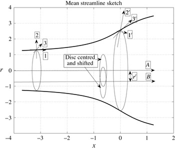
axis and passing through the point at which the velocity is to be calculated (figure 5). Using a cylindrical coordinate system
 $(r,\unicode[STIX]{x1D703},x_{1})$
, with this axis and
 $x_{1}=0$
at the disc, the vorticity field is expressed at each point of each ring element as radial, azimuthal and axial components
 $(\unicode[STIX]{x1D701}_{r},\unicode[STIX]{x1D701}_{\unicode[STIX]{x1D703}},\unicode[STIX]{x1D701}_{x1})$
. Using this system the axial velocity
 $u_{1}$
(0,0,0) depends only on the azimuthal vorticity component
 $\unicode[STIX]{x1D701}_{\unicode[STIX]{x1D703}}$
. However any given ring in the flow field will have arrived at its position from its initial state far upstream after convection and distortion by the mean flow field. If its end state is circular its initial state in general cannot have been so because of the non-uniform distortion in transit. The exception to this is when the mean flow field is also coaxial with the
 $(r,\unicode[STIX]{x1D703},x_{1})$
axis which is the case when the velocity is to be calculated at the centre of the disc. The rings of vorticity are then only subject to radial expansion and axial displacement as a whole as they are convected. The initial and final states are both circular and are simply related by a radius ratio
 $r/r_{\infty }$
and their axial
 $x_{1}$
coordinates. The
 $\unicode[STIX]{x1D701}_{r}$
and
 $\unicode[STIX]{x1D701}_{x1}$
components will both be stretched and subject to displacement from their undistorted positions, but since, although distorted, they remain in the
 $[r,x_{1}]$
plane, neither of them contribute to the axial velocity induced at (0,0,0). The
 $\unicode[STIX]{x1D701}_{\unicode[STIX]{x1D703}}$
component is subject to stretching because the mean streamlines diverge, and to radial displacement for the same reason. It is also subject to streamwise displacement due to the slowdown of the streamwise velocity. Although
 $\unicode[STIX]{x1D701}_{\unicode[STIX]{x1D703}}$
varies with
 $\unicode[STIX]{x1D703}$
around each ring the axisymmetry of the geometry and distortion greatly simplifies the computation and this therefore is the main case which has been computed.
When the velocity is calculated at other points of the disc, radially removed from the centre, the mean flow field and hence the distortion are no longer concentric with this axis system. Since the initial state of a ring whose end state is circular will now not be circular it will include
 $\unicode[STIX]{x1D701}_{r}$
and
 $\unicode[STIX]{x1D701}_{x1}$
contributions making for much greater computational work. For these cases therefore approximate estimates of
 $u_{1}$
will be calculated.
The actuator disc model omits the mean swirl component in the wake which is small except at low tip speed ratios. The helical twisting of the
 $\unicode[STIX]{x1D701}_{x1}$
component by this swirl is therefore a relatively small effect. It only occurs in the wake, being zero everywhere outside it, and in particular upstream of the rotor. It generates a very small contribution to
 $\unicode[STIX]{x1D701}_{\unicode[STIX]{x1D703}}$
and hence to the axial velocity component of distorted turbulent velocity at the disc centre and this effect is omitted throughout. The whole of the distortion effect computed for the centreline streamwise fluctuating velocity and the majority of it for the velocity off the centreline, is due to the expansion of the rings of vorticity as they are convected towards and past the actuator disc together with a lag effect due to drift. The former intensifies the azimuthal vorticity by stretching it and the latter leads to phase changes.
3.4 Distortion of the turbulence impacting the centre of the actuator disc
The components
 $\unicode[STIX]{x1D701}_{2\infty }$
and
 $\unicode[STIX]{x1D701}_{3\infty }$
in the cross-flow plane
 $x_{1}=-\infty$
of the incident vorticity can be expressed as radial
 $\unicode[STIX]{x1D701}_{r\infty }$
and azimuthal
 $\unicode[STIX]{x1D701}_{\unicode[STIX]{x1D703}\infty }$
components at any point
 $(r_{\infty },\unicode[STIX]{x1D703})$
where
 $\unicode[STIX]{x1D703}=0$
, arbitrary when axisymmetric, is taken as aligned with the direction of the radial wavenumber
 $\unicode[STIX]{x1D70F}_{\infty }$
. Substituting from (3.18) into
 $$\begin{eqnarray}\unicode[STIX]{x1D701}_{\unicode[STIX]{x1D703}\infty }=\unicode[STIX]{x1D701}_{3\infty }\cos (\unicode[STIX]{x1D703}+\unicode[STIX]{x1D6FD})-\unicode[STIX]{x1D701}_{2\infty }\sin (\unicode[STIX]{x1D703}+\unicode[STIX]{x1D6FD}),\end{eqnarray}$$
where
 $\unicode[STIX]{x1D6FD}$
is the angle between the radial wavenumber
 $\unicode[STIX]{x1D70F}_{\infty }$
and
 $\unicode[STIX]{x1D705}_{2\infty }$
i.e. the
 $x_{2}$
axis, gives
 $$\begin{eqnarray}\hat{\unicode[STIX]{x1D701}}_{\unicode[STIX]{x1D703}\infty }=\text{i}\unicode[STIX]{x1D70F}_{\infty }\hat{u} _{1\infty }\cos \unicode[STIX]{x1D703}-\frac{\text{i}\unicode[STIX]{x1D705}_{1\infty }}{\unicode[STIX]{x1D70F}_{\infty }}\{(\unicode[STIX]{x1D705}_{2\infty }\cos \unicode[STIX]{x1D703}-\unicode[STIX]{x1D705}_{3\infty }\sin \unicode[STIX]{x1D703})\hat{u} _{2\infty }+(\unicode[STIX]{x1D705}_{2\infty }\sin \unicode[STIX]{x1D703}+\unicode[STIX]{x1D705}_{3\infty }\cos \unicode[STIX]{x1D703})\hat{u} _{3\infty }\}\end{eqnarray}$$
 $\unicode[STIX]{x1D701}_{\unicode[STIX]{x1D703}}$
at a general point
 $(r,\unicode[STIX]{x1D703},x_{1})$
is therefore related as a result of stretching and radial displacement by the mean flow field of the disc to its far upstream value
 $\unicode[STIX]{x1D701}_{\unicode[STIX]{x1D703}\infty }$
by
 $$\begin{eqnarray}\hat{\unicode[STIX]{x1D701}}_{\unicode[STIX]{x1D703}}(r,\unicode[STIX]{x1D703},x_{1})=\frac{r}{r_{\infty }(r,x_{1})}\hat{\unicode[STIX]{x1D701}}_{\unicode[STIX]{x1D703}\infty }(r_{\infty },\unicode[STIX]{x1D703},-\infty ),\end{eqnarray}$$
where
 $r_{\infty }$
is the radial coordinate far upstream of the streamline passing through
 $(r,\unicode[STIX]{x1D703},x_{1})$
. Applying continuity of volume flow from far upstream
 $(-\infty )$
within the streamtube of radius
 $r$
at
 $x_{1}$
,
 $$\begin{eqnarray}\int _{0}^{r(x_{1})}2r^{\prime }\overline{U}_{1}(r^{\prime },x_{1})\,\text{d}r^{\prime }=r_{\infty }^{2}(r,x_{1}).\end{eqnarray}$$
Combined with this radial displacement from
 $r_{\infty }$
to
 $r(x_{1})$
there is an axial displacement which changes the phase of the Fourier component arriving at
 $x_{1}$
by
 $-\text{i}\unicode[STIX]{x1D705}_{1}\unicode[STIX]{x0394}x_{1}$
, where
 $$\begin{eqnarray}\unicode[STIX]{x0394}x_{1}(\unicode[STIX]{x1D6F9}(r),x_{1})=\int _{-\infty }^{x_{1}}\left(\frac{1}{\overline{U}_{1}(\unicode[STIX]{x1D6F9}(r),x_{1}^{\prime })}-1\right)\,\text{d}x_{1}^{\prime },\end{eqnarray}$$
where
 $\unicode[STIX]{x1D6F9}(r)$
is the mean flow streamline passing through
 $r(x_{1})$
.
Distortion of components of the turbulent vorticity by the mean flow: 1
 $=$
streamwise, compressed and rotated in radial plane; 2
 $=$
radial, stretched and rotated in radial plane; 3
 $=$
azimuthal, stretched;
 $A$
is the mean flow axis for
 $u_{1}$
computation at disc centre;
 $B$
is the shifted mean flow axis for
 $u_{1}$
at
 $r^{\prime }\neq 0$
(mean streamlines not indicated for this case).

This is Lighthill’s drift function discussed by Hunt (Reference Hunt1973). In the case of a planar two-dimensional body which has mean drag the far upstream velocity field is like that of a line source in a uniform flow for which the upstream perturbation only decays as
 $(-x_{1})^{-1}$
. As a result the integral forming the drift function cannot be evaluated simply and the associated phase change requires special treatment. However for an axisymmetric source-like flow the perturbation decays as
 $(-x_{1})^{-2}$
, the integral is convergent for all finite
 $x_{1}$
and a finite phase change is given directly by (3.23). (Equation (3.23) is not convergent for
 $x_{1}\rightarrow \infty$
within the far wake because
 $\overline{U}_{1}\rightarrow (1-2a)$
, but this is a limited region
 $r<1$
and has negligible effect at the rotor plane.)
Applying the Biot–Savart integral, the axial turbulent velocity induced at the disc centre
 $0$
by the distorted vorticity field is
 $$\begin{eqnarray}u_{1}(0,0,0)=-\frac{1}{4\unicode[STIX]{x03C0}}\int _{-\infty }^{\infty }\int _{-\infty }^{\infty }\int _{-\infty }^{\infty }\frac{(\unicode[STIX]{x1D701}_{2}x_{3}-\unicode[STIX]{x1D701}_{3}x_{2})}{(x_{1}^{2}+x_{2}^{2}+x_{3}^{2})^{3/2}}\,\text{d}x_{1}\,\text{d}x_{2}\,\text{d}x_{3}.\end{eqnarray}$$
Converting this into
 $(r,\unicode[STIX]{x1D703})$
coordinates:
 $$\begin{eqnarray}x_{2}=r\cos \unicode[STIX]{x1D703},\quad x_{3}=r\sin \unicode[STIX]{x1D703},\quad \unicode[STIX]{x1D701}_{2}=\unicode[STIX]{x1D701}_{r}\cos \unicode[STIX]{x1D703}-\unicode[STIX]{x1D701}_{\unicode[STIX]{x1D703}}\sin \unicode[STIX]{x1D703},\quad \unicode[STIX]{x1D701}_{3}=\unicode[STIX]{x1D701}_{r}\sin \unicode[STIX]{x1D703}+\unicode[STIX]{x1D701}_{\unicode[STIX]{x1D703}}\cos \unicode[STIX]{x1D703}\end{eqnarray}$$
 $$\begin{eqnarray}u_{1}(0,0,0)=\frac{1}{4\unicode[STIX]{x03C0}}\int _{-\infty }^{\infty }\int _{0}^{\infty }\int _{0}^{2\unicode[STIX]{x03C0}}\frac{r^{3}(p\cos \unicode[STIX]{x1D703}+q\sin \unicode[STIX]{x1D703})}{(x_{1}^{2}+r^{2})^{3/2}}\text{e}^{-\text{i}(\unicode[STIX]{x1D70F}r_{\infty }\cos \unicode[STIX]{x1D703}+\unicode[STIX]{x1D705}_{1}(x_{1}+\unicode[STIX]{x0394}x_{1})-\unicode[STIX]{x1D714}t)}\,\text{d}\unicode[STIX]{x1D703}\,\text{d}r\,\text{d}x_{1},\end{eqnarray}$$
where
 $p=\text{i}\unicode[STIX]{x1D70F}\hat{u} _{1\infty }-\text{i}(\unicode[STIX]{x1D705}_{1}\unicode[STIX]{x1D705}_{2}/\unicode[STIX]{x1D70F})\hat{u} _{2\infty }-\text{i}(\unicode[STIX]{x1D705}_{1}\unicode[STIX]{x1D705}_{3}/\unicode[STIX]{x1D70F})\hat{u} _{3\infty }$
and
 $q=\text{i}(\unicode[STIX]{x1D705}_{1}\unicode[STIX]{x1D705}_{3}/\unicode[STIX]{x1D70F})\hat{u} _{2\infty }-\text{i}(\unicode[STIX]{x1D705}_{1}\unicode[STIX]{x1D705}_{2}/\unicode[STIX]{x1D70F})\hat{u} _{3\infty }$
.
Carrying out the
 $\unicode[STIX]{x1D703}$
integration using the results that
 $$\begin{eqnarray}\displaystyle \int _{0}^{2\unicode[STIX]{x03C0}}\cos \unicode[STIX]{x1D703}\text{e}^{-\text{i}\unicode[STIX]{x1D70F}r_{\infty }\cos \unicode[STIX]{x1D703}}\,\text{d}\unicode[STIX]{x1D703}=2\unicode[STIX]{x03C0}\text{i}\text{J}_{1}(\unicode[STIX]{x1D70F}r_{\infty }) & & \displaystyle\end{eqnarray}$$
 $$\begin{eqnarray}\displaystyle \int _{0}^{2\unicode[STIX]{x03C0}}\sin \unicode[STIX]{x1D703}\text{e}^{-\text{i}\unicode[STIX]{x1D70F}r_{\infty }\cos \unicode[STIX]{x1D703}}\,\text{d}\unicode[STIX]{x1D703}=0 & & \displaystyle\end{eqnarray}$$
and
 $$\begin{eqnarray}\unicode[STIX]{x1D705}_{2}\hat{u} _{2\infty }+\unicode[STIX]{x1D705}_{3}\hat{u} _{3\infty }=-\unicode[STIX]{x1D705}_{1}\hat{u} _{1\infty }\end{eqnarray}$$
from the condition for divergence-free flow, therefore at the centre of the disc
 $$\begin{eqnarray}\displaystyle & \displaystyle u_{1}=\frac{\hat{u} _{1\infty }}{2}\int _{-\infty }^{\infty }\int _{0}^{\infty }\frac{\unicode[STIX]{x1D705}^{2}r^{2}f(r,x_{1})\text{J}_{1}\left(\displaystyle \frac{\unicode[STIX]{x1D70F}r}{f}\right)}{\unicode[STIX]{x1D70F}(x_{1}^{2}+r^{2})^{3/2}}\text{e}^{-\text{i}\unicode[STIX]{x1D705}_{1}(x_{1}+\unicode[STIX]{x0394}x_{1})}\text{e}^{\text{i}\unicode[STIX]{x1D714}t}\,\text{d}r\,\text{d}x_{1}=I_{D}\hat{u} _{1\infty }\text{e}^{\text{i}\unicode[STIX]{x1D714}t} & \displaystyle\end{eqnarray}$$
 $$\begin{eqnarray}\displaystyle & \displaystyle I_{D}=\frac{1}{2}\int _{-\infty }^{\infty }\int _{0}^{\infty }\frac{\unicode[STIX]{x1D705}^{2}r^{2}f(r,x_{1})\text{J}_{1}\left(\displaystyle \frac{\unicode[STIX]{x1D70F}r}{f}\right)}{\unicode[STIX]{x1D70F}(x_{1}^{2}+r^{2})^{3/2}}\text{e}^{-\text{i}\unicode[STIX]{x1D705}_{1}(x_{1}+\unicode[STIX]{x0394}x_{1})}\,\text{d}r\,\text{d}x_{1}. & \displaystyle\end{eqnarray}$$
In (3.30)
 $f(r,x_{1})$
is the stretching factor
 $r/r_{\infty }$
and
 $\text{J}_{1}$
is a Bessel function of the first kind.
In the event that the rotor is absent or equivalently the induction factor
 $a=0$
there will be no distortion of the incident turbulence. In that case
 $f=1$
,
 $\unicode[STIX]{x0394}x_{1}=0$
and making use of integral results (Gradshteyn & Ryzhik (Reference Gradshteyn and Ryzhik1980), integrals 3.771(2), 6.521(2))
 $$\begin{eqnarray}\frac{1}{2}\int _{-\infty }^{\infty }\int _{0}^{\infty }\frac{\unicode[STIX]{x1D705}^{2}r^{2}\text{J}_{1}(\unicode[STIX]{x1D70F}r)}{\unicode[STIX]{x1D70F}(x_{1}^{2}+r^{2})^{3/2}}\text{e}^{-\text{i}\unicode[STIX]{x1D705}_{1}x_{1}}\,\text{d}r\,\text{d}x_{1}=1\end{eqnarray}$$
from which
 $$\begin{eqnarray}u_{1}=\hat{u} _{1\infty }\text{e}^{\text{i}\unicode[STIX]{x1D714}t},\end{eqnarray}$$
which is consistent with there being no distortion.
The main difficulty with the Biot–Savart integration method is the slow convergence of the radial integral when the wavenumber
 $\unicode[STIX]{x1D70F}$
is small. Computation of this can be speeded up by subtracting (3.32) from (3.30) and therefore only numerically integrating the difference between the distorted and undistorted vorticity. This integrand
 $\rightarrow 0$
rapidly as
 $r\rightarrow \infty$
so that the radial integral converges much more rapidly.
3.5 Computation of spectra and intensities of the distorted turbulence
Having evaluated
 $\hat{u} _{1,0}$
from (3.30) above, velocity spectra and intensities of the distorted turbulence at the disc centre can be computed by integrating over the wavenumbers
 $\unicode[STIX]{x1D705}_{2}$
and
 $\unicode[STIX]{x1D705}_{3}$
, as for the small length scale case
 $$\begin{eqnarray}\unicode[STIX]{x1D719}_{11}(\unicode[STIX]{x1D705}_{1})=\frac{1}{4\unicode[STIX]{x03C0}}\int _{-\infty }^{\infty }\int _{-\infty }^{\infty }\frac{E(\unicode[STIX]{x1D705})\unicode[STIX]{x1D70F}^{2}I_{D}(\unicode[STIX]{x1D705}_{1},\unicode[STIX]{x1D70F})\tilde{I} _{D}(\unicode[STIX]{x1D705}_{1},\unicode[STIX]{x1D70F})\,\text{d}\unicode[STIX]{x1D705}_{2}\,\text{d}\unicode[STIX]{x1D705}_{3}}{\unicode[STIX]{x1D705}^{4}},\end{eqnarray}$$
where
 $\tilde{()}$
indicates a complex conjugate. Converting to radial
 $(\unicode[STIX]{x1D70F})$
integration, taking account of the axisymmetry of
 $I_{D}$
 $$\begin{eqnarray}\unicode[STIX]{x1D719}_{11}(\unicode[STIX]{x1D705}_{1})=\frac{1}{2}\int _{0}^{\infty }\frac{E(\unicode[STIX]{x1D705})\unicode[STIX]{x1D70F}^{3}|I_{D}(\unicode[STIX]{x1D705}_{1},\unicode[STIX]{x1D70F})|^{2}\,\text{d}\unicode[STIX]{x1D70F}}{\unicode[STIX]{x1D705}^{4}}\end{eqnarray}$$
and integrating with respect to
 $\unicode[STIX]{x1D705}_{1}$
 $$\begin{eqnarray}\overline{u_{1}^{2}}=\frac{1}{4}\int _{0}^{\infty }\int _{0}^{\infty }\frac{E(\unicode[STIX]{x1D705})\unicode[STIX]{x1D70F}^{3}|I_{D}(\unicode[STIX]{x1D705}_{1},\unicode[STIX]{x1D70F})|^{2}\,\text{d}\unicode[STIX]{x1D70F}\,\text{d}\unicode[STIX]{x1D705}_{1}}{\unicode[STIX]{x1D705}^{4}}.\end{eqnarray}$$
Evaluation requires substitution of an expression for the energy function
 $E(\unicode[STIX]{x1D705})$
and the von Kármán distribution will be used for this as before. Therefore,
 $$\begin{eqnarray}\unicode[STIX]{x1D719}_{11}(\unicode[STIX]{x1D705}_{1})=\frac{C\overline{u_{1}^{2}}^{\infty }}{2}\int _{0}^{\infty }\frac{\unicode[STIX]{x1D70F}^{\ast 3}|I_{D}(\unicode[STIX]{x1D705}_{1},\unicode[STIX]{x1D70F})|^{2}\,\text{d}\unicode[STIX]{x1D70F}^{\ast }}{(1+\unicode[STIX]{x1D705}_{1}^{\ast 2}+\unicode[STIX]{x1D70F}^{\ast 2})^{17/6}}\end{eqnarray}$$
and
 $$\begin{eqnarray}\overline{u_{1}^{2}}=\frac{C\overline{u_{1}^{2}}_{\infty }}{g_{0}L_{1\infty }}\int _{0}^{\infty }\int _{0}^{\infty }\frac{\unicode[STIX]{x1D70F}^{\ast 3}|I_{D}(\unicode[STIX]{x1D705}_{1},\unicode[STIX]{x1D70F})|^{2}\,\text{d}\unicode[STIX]{x1D70F}^{\ast }\,\text{d}\unicode[STIX]{x1D705}_{1}^{\ast }}{(1+\unicode[STIX]{x1D705}_{1}^{\ast 2}+\unicode[STIX]{x1D70F}^{\ast 2})^{17/6}}.\end{eqnarray}$$
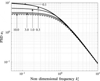
Figure 7 shows examples of the spectrum
 $\unicode[STIX]{x1D719}_{11}(\unicode[STIX]{x1D705}_{1})$
computed for the optimum value of the induction factor
 $a=1/3$
and a range of values of the length scale ratio from 0.1 to 10.0, the curves for 0.1 and 0.3 being hardly distinguishable in the log plot.
PSD of
 $u_{1}(0)$
versus frequency
 $k_{1}^{\ast }$
non-dimensionalised by
 $L_{1\infty }$
of turbulent axial velocity at the centre of the actuator disc. Distorted (solid lines)
 $L_{1\infty }=0.1,0.3,1.0,3.0,10.0$
as indicated top to bottom at left (0.1 and 0.3 curves are indistinguishable), undistorted (dashed line).

The PSD of both the undistorted and distorted spectra are approximately flat for low frequencies,
 $\unicode[STIX]{x1D705}_{1}<O(1)$
, followed by a
 $\unicode[STIX]{x1D705}_{1}^{-5/3}$
asymptotic behaviour as
 $\unicode[STIX]{x1D705}_{1}^{\ast }\rightarrow \infty$
. Therefore, the effect of distortion on the lower frequency range of the spectrum is characterised approximately by the ratio of the distorted to undistorted zero frequency intercepts:
 $$\begin{eqnarray}\unicode[STIX]{x1D6EC}=\frac{\unicode[STIX]{x1D719}_{11}(\unicode[STIX]{x1D705}_{1}^{\ast }=0)}{\unicode[STIX]{x1D719}_{11\infty }(\unicode[STIX]{x1D705}_{1}^{\ast }=0)}.\end{eqnarray}$$
The ratio
 $\unicode[STIX]{x1D6EC}$
can be computed relatively easily by setting
 $\unicode[STIX]{x1D705}_{1}=0$
in (3.37) and is plotted in figure 8 against length scale
 $L_{1\infty }$
. Its value when
 $L_{1\infty }\rightarrow 0$
is consistent with
 $\unicode[STIX]{x1D6EC}=(1-a)^{-2}$
given by the BP homogeneous strain analysis for
 $L_{1\infty }=0$
. It is notable in this figure that
 $\unicode[STIX]{x1D6EC}$
increases initially with increasing
 $L_{1\infty }$
from its value at
 $L_{1\infty }=0$
reaching a maximum at
 $L_{1\infty }\simeq 0.3$
and then decreasing thereafter to slowly approach the large length scale asymptotic value of 1.0.
Variation of zero frequency intercept ratio, distorted to undistorted, against
 $L_{1}$
.

In the same way as was done in the small length scale case the intensity of the distorted to undistorted turbulence can be evaluated by integrating the spectra over
 $\unicode[STIX]{x1D705}_{1}$
. The results of this are shown in figure 9. Also the ratio of the transverse length scales,
 $L_{2}/L_{2\infty }$
, of distorted to undistorted streamwise velocity of the turbulence can similarly be calculated, requiring integration over
 $\unicode[STIX]{x1D705}_{1}$
and one transverse wavenumber while setting the other to 0, or equivalently formulating the integral in terms of the transverse radial wavenumber
 $\unicode[STIX]{x1D70F}$
. However evaluation of
 $L_{2}$
requires spatial integration of a correlation function involving the distortion integral
 $I_{D}$
, equation (3.30), over the radius
 $r$
in the disc plane. Evaluation of
 $I_{D}(r)$
cannot then make use of the axisymmetric simplification and as a result is much more expensive computationally. In order to retain simplicity in assessing the magnitude of
 $L_{2}$
here,
 $I_{D}$
and
 $\unicode[STIX]{x0394}x_{1}$
have been approximated by their values at the disc centre, but the factor
 $\text{e}^{\text{i}\unicode[STIX]{x1D70F}r/f}$
which is the strongest influence on the correlation at given
 $y$
(or
 $r$
), is not approximated in this way. As before for general length scale cases both the distorted intensity and transverse length scale depend on the form of the undistorted spectrum but it is unlikely that the results would change significantly if the assumed spectral distribution were changed.
Evaluating the transverse length scale at the disc centre:
 $$\begin{eqnarray}\displaystyle L_{2} & = & \displaystyle \frac{\displaystyle \int _{0}^{\infty }\overline{u_{1}(0)\cdot u_{1}(y)}\,\text{d}y}{\overline{u_{1}^{2}}(0)}\nonumber\\ \displaystyle & = & \displaystyle \frac{\displaystyle \int _{0}^{\infty }\int _{-\infty }^{\infty }\int _{-\infty }^{\infty }\int _{-\infty }^{\infty }\unicode[STIX]{x1D731}_{11\infty }(\unicode[STIX]{x1D705})|I_{D}(\unicode[STIX]{x1D70F})|^{2}\text{e}^{\text{i}(\unicode[STIX]{x1D705}_{2}y/f)}\,\text{d}\unicode[STIX]{x1D73F}\,\text{d}y}{\overline{u_{1}^{2}(0)}}.\end{eqnarray}$$
The
 $y$
integration is infinite when
 $\unicode[STIX]{x1D705}_{2}=0$
, giving a Dirac delta function of
 $\unicode[STIX]{x1D705}_{2}$
which is integrated separately. The finite part of the integral is then integrated by converting it to axisymmetric form. Hence, using the von Kármán form for the energy distribution:
 $$\begin{eqnarray}\frac{L_{2}}{L_{1\infty }}=\frac{\displaystyle \int _{0}^{\infty }\int _{-\infty }^{\infty }\frac{g_{0}\unicode[STIX]{x1D70F}^{\ast 2}|I_{D}(\unicode[STIX]{x1D70F})|^{2}\,\text{d}\unicode[STIX]{x1D705}_{1}^{\ast }\,\text{d}\unicode[STIX]{x1D70F}^{\ast }}{(1+\unicode[STIX]{x1D705}_{1}^{\ast 2}+\unicode[STIX]{x1D70F}^{\ast 2})^{17/6}}+\int _{0}^{\infty }\int _{-\infty }^{\infty }\frac{\unicode[STIX]{x1D70F}^{\ast 3}|I_{D}(\unicode[STIX]{x1D70F})|^{2}I_{y}(\unicode[STIX]{x1D70F})\,\text{d}\unicode[STIX]{x1D705}_{1}^{\ast }\,\text{d}\unicode[STIX]{x1D70F}^{\ast }}{(1+\unicode[STIX]{x1D705}_{1}^{\ast 2}+\unicode[STIX]{x1D70F}^{\ast 2})^{17/6}}}{\displaystyle \int _{0}^{\infty }\int _{-\infty }^{\infty }\frac{\unicode[STIX]{x1D70F}^{\ast 3}|I_{D}(\unicode[STIX]{x1D70F})|^{2}\,\text{d}\unicode[STIX]{x1D705}_{1}^{\ast }\,\text{d}\unicode[STIX]{x1D70F}^{\ast }}{(1+\unicode[STIX]{x1D705}_{1}^{\ast 2}+\unicode[STIX]{x1D70F}^{\ast 2})^{17/6}}}\end{eqnarray}$$
with
 $$\begin{eqnarray}\frac{L_{2}}{L_{2\infty }}=2\frac{L_{2}}{L_{1\infty }}.\end{eqnarray}$$
Here
 $$\begin{eqnarray}I_{y}(\unicode[STIX]{x1D70F})=\int _{0}^{\infty }\left\{J_{0}\left(\frac{\unicode[STIX]{x1D70F}y}{f(y)}\right)-\text{J}_{0}(\unicode[STIX]{x1D70F}y)\right\}\frac{\text{d}y}{L_{1\infty }}\end{eqnarray}$$
and
 $\text{J}_{0}$
is a Bessel function of the first kind.
In the limit
 $L_{1\infty }\rightarrow 0$
the integrals for the spectra, intensity and transverse length scales, equations (3.37), (3.38) and (3.41) take their dominant contribution from the region
 $\unicode[STIX]{x1D70F}^{\ast },\unicode[STIX]{x1D705}_{1}^{\ast }\sim 1$
and therefore
 $\unicode[STIX]{x1D70F},\unicode[STIX]{x1D705}_{1}\sim \infty$
. In that case the double integral
 $I_{D}(\unicode[STIX]{x1D70F})$
given in (3.31) can be shown to take the value
 $$\begin{eqnarray}I_{D}(\unicode[STIX]{x1D70F})=\frac{\unicode[STIX]{x1D705}^{2}}{\unicode[STIX]{x1D70F}(c^{-2}\unicode[STIX]{x1D705}_{1}^{2}+c\unicode[STIX]{x1D70F}^{2})}\end{eqnarray}$$
and as a result, with
 $s=c^{-3}-1$
,
 $$\begin{eqnarray}\displaystyle & \displaystyle \frac{\overline{u_{1}^{2}}}{\overline{u_{1\infty }^{2}}}\rightarrow \frac{3(\sqrt{s}+(s-1)\tan ^{-1}\sqrt{s})}{4c^{2}s^{3/2}} & \displaystyle\end{eqnarray}$$
 $$\begin{eqnarray}\displaystyle & \displaystyle \frac{L_{2}}{L_{2\infty }}\rightarrow \frac{4cs^{3/2}}{3(\sqrt{s}+(s-1)\tan ^{-1}\sqrt{s})} & \displaystyle\end{eqnarray}$$
as
 $L_{1\infty }\rightarrow 0$
which agree with the values obtained in the
 $L_{1\infty }=0$
BP analysis.
Figure 9 shows a plot of
 $L_{2}/L_{2\infty }$
for several values of the integral length scale
 $L_{1\infty }$
when the induction factor
 $a=1/3$
. The increase in
 $L_{2}$
due to this distortion is therefore small (
 ${<}5\,\%$
when
 $L_{1\infty }>1.0$
) with
 $a=1/3$
. This would seem to agree with measurements of the transverse correlation coefficient
 $R_{11}(y)$
by Hancock & Pascheke (Reference Hancock and Pascheke2014) who found little measurable change for turbulence with
 $L_{1\infty }>1.0$
.
Variation of
 $(\overline{u_{1}^{2}}/\overline{u_{1\infty }^{2}})$
(o) and
 $(L_{2}/L_{2\infty })$
(+) with integral length scale
 $L_{1\infty },a=1/3,r=0$
.

3.6 Distorted turbulence intensity off the axis
Evaluating the distorted turbulent velocity at a general point
 $(r^{\prime },\unicode[STIX]{x1D703}^{\prime },0)$
away from the axis the simplifications resulting from axisymmetry can no longer be applied. As a result the distortion of all components of the incident vorticity must be considered in the full three-dimensional space and the computations are correspondingly orders of magnitude more intensive. As an alternative here an estimate has been made of the distortion of the streamwise component of the turbulence away from the axis. In the analysis for the small length scale limit in § 2.4 it was noted that the combined rotation angle
 $\unicode[STIX]{x1D6FD}+\unicode[STIX]{x1D6FF}$
for the mean flow through the actuator disc was small except close to the tip region and therefore in making this estimate the effect of this angle on tilting the vorticity components is ignored. It is then convenient if the
 $(r,\unicode[STIX]{x1D703},x_{1})$
axis system used in § 3.3 for axisymmetric distortion is retained passing through the selected point
 $(r^{\prime },\unicode[STIX]{x1D703}^{\prime },0)$
of the actuator disc where the distorted streamwise turbulent velocity is to be estimated. In this axis system the actuator disc itself and its mean flow field which are concentric with axis B in figure 6, are therefore shifted radially by an amount
 $r^{\prime }$
off the
 $r=0$
axis in a direction which can be taken to be
 $\unicode[STIX]{x1D703}=0$
since the distortion is independent of
 $\unicode[STIX]{x1D703}^{\prime }$
and the velocity point is retained at (0,0,0). As before, only components of vorticity which are directed azimuthally around rings concentric with the
 $r=0$
axis contribute to the velocity at (0,0,0). But each such ring in the vicinity of the disc will now have been subject to a mean strain field no longer concentric with the ring’s axis which therefore varies with
 $\unicode[STIX]{x1D703}$
around the ring. This strain field introduces contributions from
 $\unicode[STIX]{x1D701}_{r}$
and
 $\unicode[STIX]{x1D701}_{x1}$
and phase differences. These will be ignored here for the purposes of making an estimate, since the effect of the combination of tilting and drift gradients was found to be small in the small length scale case except in the tip region, § 2.4. Also it will be assumed that the velocity induced by the azimuthal vorticity can be satisfactorily estimated from the average around each ring of the pure strain component of the strain tensor to which it has been subjected. Thus, in (3.30)
 $f(r,x_{1})$
is replaced
 $\overline{f}(r,x_{1})=(1/2\unicode[STIX]{x03C0})\int _{0}^{2\unicode[STIX]{x03C0}}f(r,\unicode[STIX]{x1D703},x_{1})\,\text{d}\unicode[STIX]{x1D703}$
and
 $\unicode[STIX]{x0394}x_{1}(r,x_{1})$
is replaced by
 $\overline{\unicode[STIX]{x0394}x_{1}}(r,x_{1})=(1/2\unicode[STIX]{x03C0})\int _{0}^{2\unicode[STIX]{x03C0}}\unicode[STIX]{x0394}x_{1}(r,\unicode[STIX]{x1D703},x_{1})\,\text{d}\unicode[STIX]{x1D703}$
the average values of the stretching function
 $f$
and the drift
 $\unicode[STIX]{x0394}x_{1}$
around each ring. Therefore,
 $$\begin{eqnarray}u_{1}=\frac{\hat{u} _{1\infty }}{2}\int _{-\infty }^{\infty }\int _{0}^{\infty }\frac{\unicode[STIX]{x1D705}^{2}r^{2}\overline{f}\text{J}_{1}\left(\displaystyle \frac{\unicode[STIX]{x1D70F}r}{\overline{f}}\right)}{\unicode[STIX]{x1D70F}(x_{1}^{2}+r^{2})^{3/2}}\text{e}^{-\text{i}\unicode[STIX]{x1D705}_{1}(x_{1}+\overline{\unicode[STIX]{x0394}x_{1}})}\text{e}^{\text{i}\unicode[STIX]{x1D714}t}\,\text{d}r\,\text{d}x_{1}.\end{eqnarray}$$
Equation (3.47) is essentially the same as (3.30) except that the functions
 $f$
and
 $\unicode[STIX]{x0394}x_{1}$
are replaced by precalculated ring averages over
 $\unicode[STIX]{x1D703}$
. The computations may then be repeated to provide estimates of the distortion of the streamwise turbulent intensity at points along a radius of the actuator disc converging to the previously computed value at the centre. Estimates at four radial distances from the centre have been calculated by this procedure when
 $a=1/3$
and are shown in figure 10. There is a gradual reduction in intensity with increasing radius, with an increased rate of fall off as the tip region is approached.
Radial variation of distorted streamwise intensity for
 $L_{1\infty }/R=1.0$
and
 $a=1/3$
.

4 Distortion of mean wake vorticity by incident turbulence
The effect of terms [
 $B$
] and [
 $D$
] in (3.9) are now considered. Because the mean wake vorticity is independent of
 $x_{1}$
and is axisymmetric it does not register any axial or azimuthal displacement and therefore the only perturbation is due to its radial displacement which stretches
 $\overline{\unicode[STIX]{x1D701}}_{\unicode[STIX]{x1D703}}$
and changes its radial location.
To compute the effect of this requires a similar procedure to that followed in § 3 for the effects of distortion of the turbulence vorticity. However it is possible to estimate the general magnitude of the effect on either the zero frequency intercept or a value for some typical non-zero frequency. By considering either the turbulence components
 $u_{2}$
and
 $u_{3}$
around the wake vortex sheet or equivalently, continuity of the area integral of axial velocity
 $u_{1}$
over the cross-section of the wake, averaging this rate of radial displacement with respect to
 $\unicode[STIX]{x1D703}$
and integrating the contribution from each cross-section of the wake sheet downstream from the rotor disc, the average radial displacement
 $\unicode[STIX]{x0394}R$
of the wake at a streamwise station
 $x_{1}>0$
is found to be
 $$\begin{eqnarray}\unicode[STIX]{x0394}R\sim \hat{u} _{1}\frac{\text{J}_{1}(\unicode[STIX]{x1D70F})}{\unicode[STIX]{x1D705}_{1}\unicode[STIX]{x1D70F}}(\text{e}^{-\text{i}\unicode[STIX]{x1D702}\unicode[STIX]{x1D705}_{1}x_{1}}-1).\end{eqnarray}$$
The factor
 $\unicode[STIX]{x1D702}$
here is
 $O$
(1) and accounts for the mean convection velocity of the wake sheet, being less than the free stream speed. This stretching together with the radial displacement of the mean wake vortex sheet whose strength is
 $$\begin{eqnarray}\overline{\unicode[STIX]{x1D701}}_{\unicode[STIX]{x1D703}}=2a\end{eqnarray}$$
generates a time-dependant perturbation in the axial velocity at (0,0,0)
 $$\begin{eqnarray}u_{1w}(0)\sim a\hat{u} _{1\infty }\frac{\text{J}_{1}(\unicode[STIX]{x1D70F})}{\unicode[STIX]{x1D70F}}\left\{\unicode[STIX]{x1D706}_{0}\unicode[STIX]{x1D705}_{1}\text{K}_{1}(\unicode[STIX]{x1D706}_{0}\unicode[STIX]{x1D705}_{1})-1\right\}\text{e}^{\text{i}\unicode[STIX]{x1D714}t}.\end{eqnarray}$$
In (4.3)
 $\text{J}_{1}$
is a Bessel function of the first kind,
 $\text{K}_{1}$
is a modified Bessel function and
 $\unicode[STIX]{x1D706}_{0}~1.0$
is a factor which depends on
 $a$
.
The contribution from the distortion of the mean wake vorticity to the perturbed fluctuating streamwise velocity at the disc should be considered a part of the response of the rotor to the incident turbulence and as for the loading response of the rotor blades to the incident turbulence is part of the rotor model, not part of the incident turbulence distortion. Therefore it will not be included in the present assessment of distortion. However it is relevant to note that the above estimate indicates that it is a relatively small effect which tends to reduce the effect of the incident turbulence distortion slightly. At its largest relative to the rest of the turbulence distortion
 $|u_{1w}(0)|\sim 10\,\%$
of the latter, when
 $L_{1\infty }\sim 1$
and the Fourier components satisfy
 $\unicode[STIX]{x1D705}_{1}\sim 1$
and
 $\unicode[STIX]{x1D70F}\ll 1$
, and
 $|u_{1w}(0)|\rightarrow 0$
at either end of the
 $\unicode[STIX]{x1D705}_{1}$
range,
 $\unicode[STIX]{x1D705}_{1}\ll 1$
or
 $\unicode[STIX]{x1D705}_{1}\gg 1$
.
5 Distortion of an incident mean wake flow
The mean flow field of a wake incident from upstream may be considered to be a zero frequency
 $(\unicode[STIX]{x1D705}_{1}=0)$
convected disturbance treatable by RDT as if a component of turbulence with a deterministic distribution of transverse wavenumbers
 $\unicode[STIX]{x1D705}_{2}$
and
 $\unicode[STIX]{x1D705}_{3}$
. Prandtl (Reference Prandtl1933) in his original work on distortion of turbulence in wind tunnels modelled general turbulence by zero frequency disturbances for the purposes of calculating the distortion effects. Linearised Rapid Distortion theory is applicable for incident wakes as for turbulence if the disturbance, which is here the mean wake deficit
 $\unicode[STIX]{x0394}\overline{U}$
, is weak, i.e.
 $\unicode[STIX]{x0394}\overline{U}\ll \overline{U}$
.
The completely axisymmetric case when the wake is coaxial with the downstream rotor is considered here as an example as it is the simplest to compute. The mean wake distortion in this case is relevant for power calculations but not for unsteady forces which do not arise from this source in the perfectly coaxial case. Cases in which the incident wake is off axis can also be calculated following the same method but with rather greater computational effort. An axisymmetric wake disturbance, coaxial with the rotor, is assumed here to have the form
 $$\begin{eqnarray}\unicode[STIX]{x0394}\overline{U}_{1}(r)=-\unicode[STIX]{x1D6FC}\text{e}^{-\unicode[STIX]{x03C0}(r/R_{w})^{2}},\end{eqnarray}$$
where
 $R_{w}$
is the effective radius of the wake and
 $\unicode[STIX]{x1D6FC}$
is the velocity deficit on the centre-line.
From this, in wavenumber space
 $$\begin{eqnarray}\hat{u} _{1\infty }(\unicode[STIX]{x1D705}_{2},\unicode[STIX]{x1D705}_{3})=-\unicode[STIX]{x1D6FC}R_{w}^{2}\exp \left(-\frac{\unicode[STIX]{x1D70F}^{2}R_{w}^{2}}{4\unicode[STIX]{x03C0}}\right)\end{eqnarray}$$
and
 $\unicode[STIX]{x1D705}_{1}=0$
. Hence, following the previous analysis for general wavenumber components of turbulence,
 $$\begin{eqnarray}\displaystyle & \displaystyle \overline{U}_{1}(0,r)=1-\frac{\unicode[STIX]{x1D6FC}R_{w}^{2}}{2\unicode[STIX]{x03C0}}\int _{0}^{\infty }\unicode[STIX]{x1D70F}I_{D}(0,\unicode[STIX]{x1D70F})\text{J}_{0}(\unicode[STIX]{x1D70F}r)\exp \left(-\frac{\unicode[STIX]{x1D70F}^{2}R_{w}^{2}}{4\unicode[STIX]{x03C0}}\right)\,\text{d}\unicode[STIX]{x1D70F} & \displaystyle\end{eqnarray}$$
 $$\begin{eqnarray}\displaystyle & \displaystyle \overline{U}_{1}(0,0)=1-\frac{\unicode[STIX]{x1D6FC}R_{w}^{2}}{2\unicode[STIX]{x03C0}}\int _{0}^{\infty }\unicode[STIX]{x1D70F}I_{D}(0,\unicode[STIX]{x1D70F})\exp \left(-\frac{\unicode[STIX]{x1D70F}^{2}R_{w}^{2}}{4\unicode[STIX]{x03C0}}\right)\,\text{d}\unicode[STIX]{x1D70F}. & \displaystyle\end{eqnarray}$$
The result for an axisymmetric wake with centreline velocity defect
 $\unicode[STIX]{x1D6FC}=0.25$
and wake radius
 $R_{w}=1$
is shown in figure 11.
Distortion of an axisymmetric wake with non-dimensional mean velocity defect
 $=$
0.25 versus induction factor
 $a$
.

Prandtl (Reference Prandtl1933) assumed homogeneous mean strain acting on small length scale turbulence and obtained for distortion of streamwise velocity disturbances that
 $$\begin{eqnarray}\frac{\overline{u_{1}^{2}}}{\overline{u_{1}^{2}}_{\infty }}=c^{-2}.\end{eqnarray}$$
If the same assumption is made for the present case of the axisymmetric wake
 $(\unicode[STIX]{x1D705}_{1}=0)$
disturbance that the upstream wake width is much smaller than the downstream rotor diameter it can be seen that the distortion integral
 $I_{D}(\unicode[STIX]{x1D705}_{1}=0,\unicode[STIX]{x1D70F})$
becomes proportional to the square of the streamline divergence factor
 $f(=c^{-1/2})$
. Therefore,
 $\overline{u_{1}^{2}}\propto c^{-2}$
and hence
 $$\begin{eqnarray}\frac{\overline{u_{1}^{2}}}{\overline{u_{1\infty }^{2}}}=c^{-2},\end{eqnarray}$$
which is the same as Prandtl’s result.
6 Discussion
The behaviour overall of the spectra of the distorted turbulence is qualitatively similar to that found for turbulence interacting with bluff bodies, e.g. Hunt (Reference Hunt1973), the PSD, particularly at the low frequency end, and the intensity being increased by the distortion, the more so the smaller the integral length scale of the turbulence. But in the turbine rotor case as the integral length scale
 $L_{1\infty }$
decreases the frequency spectra
 $\unicode[STIX]{x1D719}_{11}(\unicode[STIX]{x1D705}_{1})$
in the low frequency region and the intensity ratio of the distorted turbulent axial velocity at the rotor centre both reach a maximum before the zero length scale limit is reached, around
 $L_{1\infty }\simeq 0.3$
and then decrease slightly to their (BP,
 $L_{1\infty }=0$
) values. The reason for the small initial increase as length scale increases from zero is due to the fact that the second derivative
 $\unicode[STIX]{x2202}^{2}/\unicode[STIX]{x2202}x_{1}^{2}$
of the integrand of
 $I_{D}$
is positive rather than zero at the disc plane due to the nonlinearity of the vortex stretching by the diverging streamlines passing through the disc. The major effect is the stretching function
 $f$
. At the disc centre the second derivative of
 $f$
which is the main contribution can be easily evaluated from the mean velocity on the axis as
 $$\begin{eqnarray}\frac{\text{d}^{2}f}{\text{d}x_{1}^{2}}=\frac{3a^{2}}{4(1-a)^{5/2}},\end{eqnarray}$$
which equals
 $0.23$
when
 $a=1/3$
.
The region dominating the contribution to the integral with respect to
 $x_{1}$
is
 $-L_{1\infty }<x_{1}<L_{1\infty }$
and hence as
 $L_{1\infty }$
increases initially from zero the increase from the downstream contribution is greater than the decrease from the upstream contribution. The effect is only dominant while the length scale is small enough. It occurs here because, unlike solid bodies where there is no through flow, distortion is predicted due to the flow on both sides of the rotor plane, but it is unlikely to be realistic for the turbulence in the near wake of a real rotor.
At the other end of the length scale range,
 $L_{1\infty }\rightarrow \infty$
, the values appear to approach the asymptotic undistorted values quite slowly. The high frequency behaviour of the spectra is similar to other distortions, the PSDs all following the
 $-5/3$
power behaviour. They all lie within the accuracy of the computation between the BP
 $L_{1\infty }=0$
line which has an amplification factor of
 $c^{4}\cdot \,_{2}F_{1}(2,2;17/6;1-c^{3}),=1.033$
when
 $a=1/3$
, given by (2.20), and the undistorted spectrum. The value of 1.033 is approximately the maximum value of this amplification factor which decreases either side equalling 1.0 when
 $a=0$
.
The mean streamlines through and around a turbine actuator disc diverge and it may therefore be expected that this will cause a similar extension of the transverse length scale
 $L_{2}$
. For very small length scales the BP analysis predicts, equation (2.23), that
 $$\begin{eqnarray}\frac{L_{2}}{L_{2\infty }}\rightarrow 1.118,\end{eqnarray}$$
when
 $a=1/3$
. This is less than the transverse divergence
 $(=(1-a)^{-1/2})$
of the streamlines passing through the centre region of the disc.
If 10 % change in r.m.s. force and 20 % change in power is taken as the minimum significant distortion effect, the computed results indicate that for normal operating conditions
 $(a=1/3)$
distortion is not significant if the non-dimensional length scale
 $L_{1\infty }>2$
, i.e. the integral length scale of the turbulence is greater than the diameter of the turbine. Figure 8 indicates a stronger effect of distortion than this on the low frequency content of the spectrum. This is a consideration only for slow variations in force on the rotor and possible increases in the power generated than of any significance in the unsteady buffeting regime. To set these frequencies in perspective the rotational frequency of a wind or tidal turbine rotor under usual operating conditions corresponds to a non-dimensional frequency
 $k_{1}^{\ast }\propto L_{1\infty }$
where the constant of proportionality is of order the tip speed ratio and therefore of order 10. The blade passing frequency is higher by a factor equal to the number of blades (almost always 2 or 3). Both these frequencies lie well above the main amplification region of the spectra indicated in figure 7 unless the turbulence length scale is small as perhaps in wind farm wake-generated turbulence rather than ABL turbulence. The actuator disc model of mean flow through the rotor is not valid for frequencies near or above these frequencies since detailed flow around individual blades then becomes relevant, but the indication would seem to be that distortion is not significant at these frequencies.
On the other hand the above criterion of relevance applied to distortion of a mean wake from an upstream rotor, in the example shown in figure 11 where the wake has an effective diameter equal to the rotor diameter and a centreline defect of
 $25\,\%$
(not untypical), indicates that distortion of the mean profile of an incident wake is significant.
7 Conclusions
This paper has applied linearised RDT to assess the magnitude of distortion effects on incident turbulence by the mean flow field of an open turbine rotor. The main calculations have been performed for the fluctuating axial velocity incident on the centreline of the rotor as this offers considerable computational simplification and estimates have been obtained for the radial variation over the rotor away from the axis. The most sensitive region of the blade to buffet loads from incident turbulence is the outer region of the blade somewhat inboard of the tip. The calculations in this paper show a gradual reduction in the distortion effect towards the rotor tip region, reducing to approximately
 $90\,\%$
of the centreline value at the tip. In the small length scale case the fall off at the tip is more pronounced. The results for arbitrary length scales tend towards the zero length scale limits given by the homogeneous RDT theory of Batchelor & Proudman (Reference Batchelor and Proudman1954) as
 $L_{1\infty }\rightarrow 0$
with a small maximum above these values when the length scale is approximately
 $15\,\%$
of the rotor diameter.
The results indicate that the effect of distortion is not significant if the integral length scale of the turbulence is larger than the rotor diameter and that the strongest effects are for the low frequency (relative to the blade-passing-frequency) end of the spectrum.
However distortion of the mean velocity profile of an incident wake from an upstream turbine, calculated for a wake impacting the rotor coaxially, can be significant due to the relatively smaller length scale of the incident disturbance in this case.
Acknowledgement
This work was supported by the Engineering and Physical Sciences Research Council (UK) through the Innovate UK project SWEPT2 which is gratefully acknowledged.