1 Introduction
The stability of an inviscid swirling flow in a circular pipe is a crucial subject for the development of various technologies such as engine nozzles, combustion chambers, hydrocyclone separators and other flow devices where swirl has a dominant influence. It also sheds light on the scientific understanding of physical phenomena of vortex flows, such as the vortex breakdown phenomenon. For reviews of this topic see Leibovich (Reference Leibovich1984) and Ash & Khorrami (Reference Ash, Khorrami and Green1995).
Stability theory of vortex flows (Kelvin Reference Kelvin1880; Rayleigh Reference Rayleigh1916; Synge Reference Synge1933; Howard & Gupta Reference Howard and Gupta1962; Lessen & Paillet Reference Lessen and Paillet1974; Lessen, Singh & Paillet Reference Lessen, Singh and Paillet1974; Leibovich & Stewartson Reference Leibovich and Stewartson1983) used classical azimuthal and axial normal mode analysis to determine the tendency of a small disturbance imposed on a swirling flow in a circular pipe to grow or decay in time. Specifically, for the case of a base solid-body rotation flow with a uniform axial speed in an infinitely long pipe, perturbations must stay bounded at the pipe upstream and downstream far-field states at
 $\pm \infty$
(the far-field conditions) and also obey the wall no-penetration condition. The linearized flow equations, together with the far-field and wall conditions, globally and completely determine the set of the perturbation modes, including the axial and azimuthal Fourier modes, and their stability characteristics. Kelvin (Reference Kelvin1880) solved analytically this linearized flow problem and found that this base flow is neutrally stable (no growth or decay of perturbations) for any axial wavenumber (
 ${\it\alpha}$
, a real number) and azimuthal wavenumber (
 $m$
, an integer) of the perturbations. He gave a dispersion formula for the frequency and axial group speed of both axisymmetric and helical perturbations as a function of
 ${\it\alpha}$
and
 $m$
(see details of this analysis also in Ash & Khorrami (Reference Ash, Khorrami and Green1995)). In the
 $m=0$
(axisymmetric) case, the wave is an axial sinusoidal wave while in the case
 $m\neq 0$
the wave is helical. We note that Di Prima & Habetler (Reference Di Prima and Habetler1969) proved a completeness theorem for the non-self adjoint eigenvalue problem derived by the classical method of normal mode analysis for a more general base flow in an infinitely long pipe. Therefore, all types of perturbations to a base solid-body rotation flow in an infinitely long pipe can be described by the normal modes or a linear combination of these modes. Moreover, since the solid-body rotation flow with a uniform axial velocity is strain free (the only swirling flow that is strain free), there is no perturbation kinetic energy exchange between the perturbation and the bulk. In the inviscid flow case, the axial periodic and circumferential periodic wave nature of the perturbations embed the neutral stability of these modes. In the viscous flow case, there is internal damping in the bulk that induces a decay of all the perturbations and an asymptotic return in time to the base flow.
However, as also shown in this paper, such an approach is limited to the case of a flow in an infinitely long pipe or a finite-length pipe with periodic inlet–outlet conditions (see also Wang & Rusak Reference Wang and Rusak2011). This limitation was overlooked in the classical stability theory for over a hundred years. The inviscid flow stability study of Wang & Rusak (Reference Wang and Rusak1996a
) was the first to reveal this crucial limitation of the classical stability theory of vortex flows for the case of axisymmetric (
 $m=0$
) perturbations to a swirling flow in a finite-length pipe. The classical normal mode analysis may not be applicable to the study of the stability of the swirling flow in a finite-length pipe with a vortex generator ahead of it, where the flow dynamics strongly interferes with the inlet and outlet states.
In the case where a swirling flow enters the pipe, after it has been generated by a fixed in place and fixed in time vortex generator, and it is discharged by a device at the pipe outlet, there may be an interference of the perturbation with the inlet and outlet states and an exchange of perturbation’s kinetic energy in the bulk through these boundary states. Wang & Rusak (Reference Wang and Rusak1996a ) introduced and studied such an influence as an essential ingredient to trigger the instability of axisymmetric perturbations to a high-swirl solid-body rotation flow in a finite-length, straight, circular pipe as the swirl level is increased. In their approach, three boundary conditions at the pipe inlet and one condition at the outlet replace the far-field conditions of the classical analysis. The linearized flow equations, together with these non-periodic inlet and outlet conditions and the wall no-penetration condition, form a different, well-defined eigenvalue problem that also globally and completely determines the set of the perturbation modes on the flow. Wang & Rusak (Reference Wang and Rusak1996a ) revealed, through an analytical solution, the existence of a continuum of eigenmodes of perturbations that are completely different from the classical normal (Kelvin) modes and that form axial wave shapes that are not sinusoidal (not Fourier modes) due to the influence of the boundary conditions set at the inlet and outlet. It was found that these modes become unstable in sequence and with increasing growth rates as the flow swirl ratio increases above a certain, critical, swirl level. Because of their role in the study of the onset of the axisymmetric vortex breakdown phenomenon, these unstable modes and their extension to the more general base swirling flows in a finite-length pipe, have been extensively studied from various aspects in the past two decades. The Wang & Rusak (Reference Wang and Rusak1996a ) physical and mathematical models and analysis were extended to describe the vortex breakdown process in Lamb–Oseen vortices (see Wang & Rusak Reference Wang and Rusak1997a and Rusak et al. Reference Rusak, Wang, Xu and Taylor2012). The axisymmetric instability modes on swirling flows under various inlet and outlet conditions were also studied by Gallaire & Chomaz (Reference Gallaire and Chomaz2004), Vyazmina et al. (Reference Vyazmina, Nichols, Chomaz and Schmid2009) and Leclaire & Sipp (Reference Leclaire and Sipp2010). The experiments of Mattner, Joubert & Chong (Reference Mattner, Joubert and Chong2002) verified some aspects of the vortex breakdown theory by Wang & Rusak (Reference Wang and Rusak1997a ); also see Rusak, Wang & Whiting (Reference Rusak, Wang and Whiting1998) for the agreement of the theoretical predictions with the Garg & Leibovich (Reference Garg and Leibovich1979) experimental results. The instability modes have been recently shown to be crucial in the evolution of small perturbations to a base solid-body rotation flow to form a breakdown process and its stabilization on either vortex breakdown or wall-separation states (see Rusak & Wang Reference Rusak and Wang2014). A similar flow evolution was recently observed in the experiments of Dennis, Seraudie & Poole (Reference Dennis, Seraudie and Poole2014). All of these studies established a solid theoretical understanding of the axisymmetric vortex breakdown process.
The pipe flow experiments of Sarpkaya (Reference Sarpkaya1971, Reference Sarpkaya1974), Faler & Leibovich (Reference Faler and Leibovich1977), Garg & Leibovich (Reference Garg and Leibovich1979) (also see Leibovich Reference Leibovich1984), Uchida & Ohsawa (Reference Uchida and Ohsawa1985), Bayomi et al. (Reference Bayomi, Said, Sedrak and Sye2011), and Dennis et al. (Reference Dennis, Seraudie and Poole2014) have shown the existence of various types of disrupted states of vortex flows and vortex breakdown. These include three-dimensional helical or spiral waves, the axisymmetric (bubble) type and the spiral type of vortex breakdown states. They found that for a fixed Reynolds number, the breakdown that first appears with the increase of swirl is the spiral type (Leibovich Reference Leibovich1984). As the swirl is further increased above a second critical value, the spiral breakdown transforms into an axisymmetric breakdown. They also found the interchange of the breakdown types in time from a spiral to an axisymmetric bubble and vice versa. In addition, the numerical simulations of Spall & Gatski (Reference Spall and Gatski1991), Spall (Reference Spall1996), Tromp & Beran (Reference Tromp and Beran1996) and Cary, Darmofal & Powell (Reference Cary, Darmofal and Powell1997) have computed the evolution of various three-dimensional spiral waves and spiral breakdown states. These phenomena are beyond the scope of the axisymmetric framework of analysis. This raises the crucial need to extend the Wang & Rusak (Reference Wang and Rusak1996a ) stability analysis to the general case of three-dimensional perturbations to a base swirling flow in a finite-length pipe with non-periodic boundary conditions at the pipe inlet and outlet. In the present paper, we focus on the solid-body rotation flow with a uniform axial velocity as a benchmark case study to reveal the existence of unstable axisymmetric and three-dimensional modes and the possible competition between these perturbations. Such a study will complete the linear stability analysis of a base solid-body rotation flow in a finite-length pipe in both the inviscid and viscous flow cases.
The present paper describes the various axisymmetric and three-dimensional instability modes that appear on a solid-body rotation flow in a finite-length straight circular pipe with boundary conditions similar to those used by Wang & Rusak (Reference Wang and Rusak1996a
). We first focus on the fundamental inviscid flow three-dimensional stability problem. The present study is a direct extension of the axisymmetric stability analysis of Wang & Rusak (Reference Wang and Rusak1996a
). As in the axisymmetric flow case, we find the existence of unstable spiral modes with various circumferential wavenumbers and axial wavelengths and with increasing values of growth rates that appear in sequence as the inlet flow swirl ratio increases above a critical swirl level. We then extend the analysis to viscous flows at various Reynolds numbers (
 $Re$
). We show that at
 $Re>300$
the viscous effects through the bulk and the pipe boundaries play only a passive role in determining the axisymmetric and spiral mode shapes and, at a fixed swirl level, they reduce the modes’ growth rates by a nearly constant value that decreases with the increase of
 $Re$
. Through the use of Reynolds–Orr equation for the perturbation’s kinetic energy, we shed light on the energy transfer mechanism that governs in the present set-up the exchange of stability of the various modes as the swirl ratio is increased.
The present paper focuses on identifying the fundamental mechanism of the three-dimensional stability of a base solid-body rotation with a uniform axial velocity in a finite-length rotating pipe in both the inviscid and the viscous flow cases. This flow can be realized in experiments using a system of a rotating honeycomb ahead of the rotating pipe of a finite short length, of the order of two to six pipe radii. The study reveals the crucial mechanism of axial inhomogeneity between the inlet and outlet boundary conditions in determining the rotating flow stability. Also, the solid-body rotation flow has no internal production of perturbation’s kinetic energy and thereby the instabilities found in the present paper are related only to the axial inhomogeneity between the inlet and outlet boundary conditions. The present work is directly related to and extends the classical stability study of Kelvin (Reference Kelvin1880) that used homogeneous symmetric upstream and downstream conditions and thus reveals the limitation of the classical theory. This is a necessary task for clarifying the relationship between the classical theory and the current theoretical development. All vortex flows in finite domains may share this axial inhomogeneity mechanism.
However, in other vortex flows, where the vortical core size is smaller than the pipe radius, viscous dissipation in the bulk and from the developing wall boundary layers may add inhomogeneity to the base flow development along the pipe. Thereby, these viscous effects serve as another source for axial inhomogeneity in the flow. As a function of Reynolds number, they modify (and in certain cases even significantly modify) the base flow structure (Wang & Rusak Reference Wang and Rusak1997b ) as well as its stability characteristics in response to both axisymmetric and three-dimensional perturbations that result from the inhomogeneity between the inlet and outlet. Wall boundary layer effects have been shown in the modified bifurcation diagrams of steady states of rotating flows by Meliga & Gallaire (Reference Meliga and Gallaire2011) with respect to those of Lopez (Reference Lopez1994) (who used a slip condition along the pipe wall). However, as shown in this paper, in the case of a solid-body rotation, the viscous effects are not a necessary ingredient to generate three-dimensional instabilities. Also, except for the solid-body rotation flow, all vortex flows include the production of perturbation’s kinetic energy in the bulk which changes the transfer of perturbation kinetic energy in response to both axisymmetric flows (as was already found by Wang & Rusak (Reference Wang and Rusak2011)) and three-dimensional perturbations (that should be further studied).
Similarly, an axisymmetric breakdown zone in the swirling flow also naturally creates an axial inhomogeneity in the flow that leads to three-dimensional instabilities and the spiral mode of breakdown. For example, Ruith et al. (Reference Ruith, Chen, Meiburg and Maxworthy2003) computed three-dimensional instabilities on a vortex breakdown state, but did not give a physical explanation for the root cause of the instabilities, as revealed in this paper. Note that Ruith et al. (Reference Ruith, Chen, Meiburg and Maxworthy2003) used similar inlet and outlet conditions but did not relate between the appearance of instabilities and the axial inhomogeneity due to these conditions. As shown in this paper, the axisymmetric breakdown zone is also not a necessary ingredient to generate three-dimensional instabilities. These instabilities can appear at swirl levels below those where breakdown zones appear, as documented in the pioneering experiments of Sarpkaya (Reference Sarpkaya1971, Reference Sarpkaya1974) and Faler & Leibovich (Reference Faler and Leibovich1977).
This point of view that axial flow inhomogeneity (from whatever source, but specifically from the inlet and outlet conditions) is the root cause for flow three-dimensional instabilities is new. It reveals and provides for the first time a consistent physical mechanism for both the axisymmetric instability (Wang & Rusak Reference Wang and Rusak1996a ,Reference Wang and Rusak b ) and the three-dimensional instability in swirling flows in a finite-length pipe, which was never established in any of the previous studies of vortex stability and breakdown.
The outline of the paper is as follows. In § 2 we derive the linear stability equations for the viscous flow case and the related boundary conditions. We note that in the inviscid flow case the present governing stability equations are the same as those used by Kelvin (Reference Kelvin1880). However, Kelvin (Reference Kelvin1880) used a complete normal mode analysis that is suitable only for a flow in an ideal infinitely long pipe. On the other hand, we study in this paper a general mode of perturbation that satisfies the inlet–outlet conditions of a flow in a finite-length pipe set-up as described above. In the inviscid flow case, the present problem reduces to a problem that is similar to that studied in Wang & Rusak (Reference Wang and Rusak1996a
) when the perturbations are axisymmetric. The stability problem for both the inviscid and viscous flow problems is solved numerically for all azimuthal wavenumbers
 $m$
. In § 3 we compare the results of computations for the case of
 $m=0$
with benchmark results based on the Wang & Rusak (Reference Wang and Rusak1996a
) analysis. For the
 $m=1$
mode, we demonstrate the convergence of computed growth rates with mesh refinement in both the inviscid and viscous flow cases. In § 4 we present the inviscid flow growth rates of the various perturbation modes as a function of the base flow swirl ratio and the related mode shapes. We find that for the azimuthal wavenumbers studied, instability modes appear in sequence as the swirl ratio is increased. In § 5 we extend the analysis to viscous flows at
 $Re=1000$
and
 $Re=500$
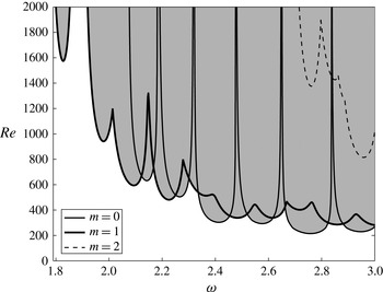
. We also present the neutral stability line in a
 $Re$
versus swirl level diagram. The
 $m=1$
instability modes compete with the axisymmetric (
 $m=0$
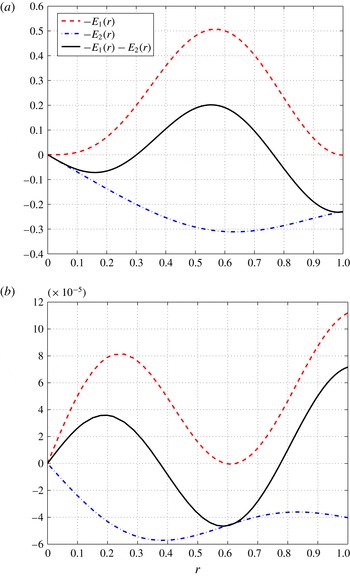
) instability modes as the inlet swirl ratio is increased. In § 6 we use the Reynolds–Orr equation to analyse the various production terms of the perturbation’s kinetic energy and establish the elimination of flow axial homogeneity in the pipe at high swirl levels as the underlying physical mechanism that leads to the flow change of stability and the appearance of both spiral and axisymmetric instabilities.
2 Formulation of the problem
We consider an incompressible swirling flow of a Newtonian fluid in a rotating, straight, finite-length circular pipe. The cylindrical polar coordinates
 $(x,r,{\it\theta})$
are used where
 $x$
is the axial distance from the pipe inlet and
 $r$
is the radial distance from the pipe centreline. The axial and radial distances are scaled with the pipe radius
 $R$
such that the pipe non-dimensional radius is unity and the pipe non-dimensional length is
 $L$
. The flow domain is given by
 $V_{C}=\{(x,r,{\it\theta}):0\leqslant x\leqslant L,0\leqslant r\leqslant 1,0\leqslant {\it\theta}<2{\rm\pi}\}$
. The velocity components are scaled with the characteristic axial speed entering the pipe, denoted
 $U$
. The non-dimensional velocity vector,
 $\boldsymbol{u}$
, is given by its axial, radial and circumferential components, respectively,
 $\boldsymbol{u}=(u_{x},u_{r},u_{{\it\theta}})$
. The flow density
 ${\it\rho}$
and fluid viscosity
 ${\it\mu}$
are constant. The gage pressure from the chamber base reference pressure is scaled with the characteristic dynamic pressure
 ${\it\rho}U^{2}$
and is denoted as
 $p$
. The time
 $t$
is scaled with the ratio of pipe radius to inlet characteristic speed. The flow inside the domain
 $V_{C}$
is described by the non-dimensional continuity and axial, radial and circumferential momentum equations,
 $$\begin{eqnarray}\displaystyle & \displaystyle \frac{\partial u_{r}}{\partial r}+\frac{u_{r}}{r}+\frac{1}{r}\frac{\partial u_{{\it\theta}}}{\partial {\it\theta}}+\frac{\partial u_{x}}{\partial x}=0,\qquad & \displaystyle\end{eqnarray}$$
 $$\begin{eqnarray}\displaystyle & \displaystyle \frac{\partial u_{x}}{\partial t}+u_{r}\frac{\partial u_{x}}{\partial r}+\frac{u_{{\it\theta}}}{r}\frac{\partial u_{x}}{\partial {\it\theta}}+u_{x}\frac{\partial u_{x}}{\partial x}=-\frac{\partial p}{\partial x}+\frac{1}{Re}\text{D}u_{x},\qquad & \displaystyle\end{eqnarray}$$
 $$\begin{eqnarray}\displaystyle & \displaystyle \frac{\partial u_{r}}{\partial t}+u_{r}\frac{\partial u_{r}}{\partial r}+\frac{u_{{\it\theta}}}{r}\frac{\partial u_{r}}{\partial {\it\theta}}+u_{x}\frac{\partial u_{r}}{\partial x}-\frac{u_{{\it\theta}}^{2}}{r}=-\frac{\partial p}{\partial r}+\frac{1}{Re}\left(\text{D}u_{r}-\frac{2}{r^{2}}\frac{\partial u_{{\it\theta}}}{\partial {\it\theta}}-\frac{u_{r}}{r^{2}}\right),\qquad & \displaystyle\end{eqnarray}$$
 $$\begin{eqnarray}\displaystyle & \displaystyle \frac{\partial u_{{\it\theta}}}{\partial t}+u_{r}\frac{\partial u_{{\it\theta}}}{\partial r}+\frac{u_{{\it\theta}}}{r}\frac{\partial u_{{\it\theta}}}{\partial {\it\theta}}+u_{x}\frac{\partial u_{{\it\theta}}}{\partial x}+\frac{u_{{\it\theta}}u_{r}}{r}=-\frac{1}{r}\frac{\partial p}{\partial {\it\theta}}+\frac{1}{Re}\left(\text{D}u_{{\it\theta}}+\frac{2}{r^{2}}\frac{\partial u_{r}}{\partial {\it\theta}}-\frac{u_{{\it\theta}}}{r^{2}}\right).\qquad & \displaystyle\end{eqnarray}$$
 $$\begin{eqnarray}\text{D}=\frac{\partial ^{2}}{\partial r^{2}}+\frac{1}{r}\frac{\partial }{\partial r}+\frac{1}{r^{2}}\frac{\partial ^{2}}{\partial {\it\theta}^{2}}+\frac{\partial ^{2}}{\partial x^{2}}\end{eqnarray}$$
is the Laplace operator in cylindrical polar coordinates and
 $Re$
is the Reynolds number,
 $Re={\it\rho}UR/{\it\mu}$
. In the inviscid flow case, the terms related to
 $1/Re$
are eliminated from the momentum equations.
The system (2.1a–d
) is subjected to certain boundary conditions that may reflect a physical setting of a flow in a straight, circular rotating pipe that is generated by a vortex generator at a steady, continuous and smooth operation ahead of the pipe inlet. In the present study we focus on a special setting where the inlet profile is a steady solid-body rotating flow with a uniform axial velocity. The non-dimensional axial, radial and azimuthal velocities at the pipe inlet,
 $x=0$
, are fixed for all time
 $t\geqslant 0$
,
 $$\begin{eqnarray}\displaystyle & \displaystyle u_{x}(0,r,{\it\theta},t)=1, & \displaystyle\end{eqnarray}$$
 $$\begin{eqnarray}\displaystyle & \displaystyle u_{r}(0,r,{\it\theta},t)=0, & \displaystyle\end{eqnarray}$$
 $$\begin{eqnarray}\displaystyle & \displaystyle u_{{\it\theta}}(0,r,{\it\theta},t)={\it\omega}r\quad \text{for }0\leqslant r\leqslant 1~\text{and}~0\leqslant {\it\theta}<2{\rm\pi}. & \displaystyle\end{eqnarray}$$
 ${\it\omega}\geqslant 0$
is the inlet flow swirl ratio. These inlet conditions may represent the nature of a swirling flow generated by a rotating honeycomb ahead of the rotating pipe (see Leclaire & Sipp Reference Leclaire and Sipp2010). Slightly different inlet conditions that may represent the case of a vortex generator that is built of guiding vanes have been studied in Wang & Rusak (Reference Wang and Rusak1996a
, Reference Wang and Rusak1997a
).
The flow is treated as being locally inviscid at the pipe wall and at the pipe outlet, see for example, Fletcher (Reference Fletcher1991) for a discussion of boundary conditions. The boundary condition at the pipe outlet,
 $x=L$
, is described by a zero axial gradient of the pressure for all time
 $t\geqslant 0$
,
 $$\begin{eqnarray}\displaystyle \frac{\partial p}{\partial x}(L,r,{\it\theta},t)=0\quad \text{for}~0\leqslant r\leqslant 1~\text{and}~0\leqslant {\it\theta}<2{\rm\pi}. & & \displaystyle\end{eqnarray}$$
This condition is supported by the experimental data shown in Umeh et al. (Reference Umeh, Rusak, Gutmark, Villalva and Cha2010) where the mean swirling flow has established a parallel flow state after several radii from the pipe inlet.
The pipe wall is modelled as an inviscid, slip boundary. At the pipe wall,
 $r=1$
, we impose the no-penetration condition for all time
 $t\geqslant 0$
,
 $$\begin{eqnarray}\displaystyle u_{r}(x,1,{\it\theta},t)=0. & & \displaystyle\end{eqnarray}$$
Beran (Reference Beran1994) and Lopez (Reference Lopez1994) have used a similar wall condition in their numerical study of viscous swirling flows in pipes.
Under the boundary conditions specified above, the solid-body rotation flow with a uniform axial velocity and no radial velocity,
 $$\begin{eqnarray}\displaystyle & \displaystyle u_{x}(x,r,{\it\theta},t)=1, & \displaystyle\end{eqnarray}$$
 $$\begin{eqnarray}\displaystyle & \displaystyle u_{r}(x,r,{\it\theta},t)=0, & \displaystyle\end{eqnarray}$$
 $$\begin{eqnarray}\displaystyle & \displaystyle u_{{\it\theta}}(x,r,{\it\theta},t)=0, & \displaystyle\end{eqnarray}$$
 $$\begin{eqnarray}\displaystyle & \displaystyle p(x,r,{\it\theta},t)={\it\omega}^{2}\frac{r^{2}}{2}\quad \text{for}~0\leqslant x\leqslant L,0\leqslant r\leqslant 1~\text{and}~0\leqslant {\it\theta}<2{\rm\pi} & \displaystyle\end{eqnarray}$$
 ${\it\omega}$
and all
 $Re$
; this is the base flow for the present linear stability analysis. The base flow non-dimensional velocity vector and gage pressure are denoted
 $\boldsymbol{u}_{0}=(1,0,{\it\omega}r)$
and
 $p_{0}(r)={\it\omega}^{2}r^{2}/2$
.
We consider small perturbations of the base velocity vector, given by
 $$\begin{eqnarray}{\it\epsilon}\boldsymbol{u}^{\prime }(x,r,{\it\theta},t)={\it\epsilon}(u_{x}^{\prime }(x,r,{\it\theta},t),u_{r}^{\prime }(x,r,{\it\theta},t),u_{{\it\theta}}^{\prime }(x,r,{\it\theta},t)),\end{eqnarray}$$
and of the pressure, given by
 ${\it\epsilon}p^{\prime }(x,r,{\it\theta},t)$
, where
 ${\it\epsilon}>0$
is a small parameter. Then,
 $$\begin{eqnarray}\displaystyle & \displaystyle \boldsymbol{u}=\boldsymbol{u}_{0}+{\it\epsilon}\boldsymbol{u}^{\prime }=(1+{\it\epsilon}u_{x}^{\prime },{\it\epsilon}u_{r}^{\prime },{\it\omega}r+{\it\epsilon}u_{{\it\theta}}^{\prime })\quad \text{and}\quad p=p_{0}+{\it\epsilon}p^{\prime }={\it\omega}^{2}\frac{r^{2}}{2}+{\it\epsilon}p^{\prime }.\qquad & \displaystyle\end{eqnarray}$$
Substituting (2.8) into the governing equations (2.1a–d
) leads, at order
 $O({\it\epsilon})$
, to the equations of the linearized flow dynamics inside the domain
 $V_{C}$
for all time
 $t\geqslant 0$
,
 $$\begin{eqnarray}\displaystyle & \displaystyle \frac{\partial u_{r}^{\prime }}{\partial r}+\frac{u_{r}^{\prime }}{r}+\frac{1}{r}\frac{\partial u_{{\it\theta}}^{\prime }}{\partial {\it\theta}}+\frac{\partial u_{x}^{\prime }}{\partial x}=0, & \displaystyle\end{eqnarray}$$
 $$\begin{eqnarray}\displaystyle & \displaystyle \frac{\partial u_{x}^{\prime }}{\partial t}+{\it\omega}\frac{\partial u_{x}^{\prime }}{\partial {\it\theta}}+\frac{\partial u_{x}^{\prime }}{\partial x}=-\frac{\partial p^{\prime }}{\partial x}+\frac{1}{Re}\text{D}u_{x}^{\prime }, & \displaystyle\end{eqnarray}$$
 $$\begin{eqnarray}\displaystyle & \displaystyle \frac{\partial u_{r}^{\prime }}{\partial t}+{\it\omega}\frac{\partial u_{r}^{\prime }}{\partial {\it\theta}}-2{\it\omega}u_{{\it\theta}}^{\prime }+\frac{\partial u_{r}^{\prime }}{\partial x}=-\frac{\partial p^{\prime }}{\partial r}+\frac{1}{Re}\left(\text{D}u_{r}^{\prime }-\frac{u_{r}^{\prime }}{r^{2}}-\frac{2}{r^{2}}\frac{\partial u_{{\it\theta}}^{\prime }}{\partial {\it\theta}}\right), & \displaystyle\end{eqnarray}$$
 $$\begin{eqnarray}\displaystyle & \displaystyle \frac{\partial u_{{\it\theta}}^{\prime }}{\partial t}+{\it\omega}\frac{\partial u_{{\it\theta}}^{\prime }}{\partial {\it\theta}}+2{\it\omega}u_{r}^{\prime }+\frac{\partial u_{{\it\theta}}^{\prime }}{\partial x}=-\frac{1}{r}\frac{\partial p^{\prime }}{\partial {\it\theta}}+\frac{1}{Re}\left(\text{D}u_{{\it\theta}}^{\prime }-\frac{u_{{\it\theta}}^{\prime }}{r^{2}}+\frac{2}{r^{2}}\frac{\partial u_{r}^{\prime }}{\partial {\it\theta}}\right). & \displaystyle\end{eqnarray}$$
We consider a suitable general mode analysis of the linearized flow problem in a straight circular pipe that is composed of an azimuthal normal mode in
 ${\it\theta}$
(since the problem preserves azimuthal symmetry) and a non-axial Fourier mode in
 $x$
and
 $r$
that must obey the non-periodic inlet–outlet conditions. This mode is given in the form:
 $$\begin{eqnarray}\displaystyle & \displaystyle u_{x}^{\prime }(x,r,{\it\theta},t)=\mathscr{W}(x,r)\text{e}^{\text{i}m{\it\theta}+{\it\sigma}t},\quad u_{r}^{\prime }(x,r,{\it\theta},t)=\mathscr{U}(x,r)\text{e}^{\text{i}m{\it\theta}+{\it\sigma}t}, & \displaystyle\end{eqnarray}$$
 $$\begin{eqnarray}\displaystyle & \displaystyle u_{{\it\theta}}^{\prime }(x,r,{\it\theta},t)=\mathscr{V}(x,r)\text{e}^{\text{i}m{\it\theta}+{\it\sigma}t},\quad p^{\prime }(x,r,{\it\theta},t)=\mathscr{P}(x,r)\text{e}^{\text{i}m{\it\theta}+{\it\sigma}t}. & \displaystyle\end{eqnarray}$$
Here
 ${\it\sigma}$
may be a complex number that relates to the growth rate of the perturbation,
 $\text{i}$
is the imaginary unit and
 $m$
is an integer representing the perturbation’s azimuthal wavenumber. The perturbation admits a separation of variables solution in terms of
 $(x,r)$
,
 ${\it\theta}$
and
 $t$
. Substituting the general mode shape (2.10) into (2.9a–d
) results for each
 $m$
in
 $$\begin{eqnarray}\displaystyle & \displaystyle \frac{\partial \mathscr{U}}{\partial r}+\frac{1}{r}\mathscr{U}+\frac{\text{i}m}{r}\mathscr{V}+\frac{\partial \mathscr{W}}{\partial x}=0, & \displaystyle\end{eqnarray}$$
 $$\begin{eqnarray}\displaystyle & \displaystyle {\it\sigma}\mathscr{W}+\text{i}m{\it\omega}\mathscr{W}+\frac{\partial \mathscr{W}}{\partial x}=-\frac{\partial \mathscr{P}}{\partial x}+\frac{1}{Re}\text{D}^{\dagger }\mathscr{W}, & \displaystyle\end{eqnarray}$$
 $$\begin{eqnarray}\displaystyle & \displaystyle {\it\sigma}\mathscr{U}+\text{i}m{\it\omega}\mathscr{U}-2{\it\omega}\mathscr{V}+\frac{\partial \mathscr{U}}{\partial x}=-\frac{\partial \mathscr{P}}{\partial r}+\frac{1}{Re}\left(\text{D}^{\dagger }\mathscr{U}-\frac{1}{r^{2}}\mathscr{U}-\frac{2m\text{i}}{r^{2}}\mathscr{V}\right), & \displaystyle\end{eqnarray}$$
 $$\begin{eqnarray}\displaystyle & \displaystyle {\it\sigma}\mathscr{V}+\text{i}m{\it\omega}\mathscr{V}+2{\it\omega}\mathscr{U}+\frac{\partial \mathscr{V}}{\partial x}=-\frac{\text{i}m}{r}\mathscr{P}+\frac{1}{Re}\left(\text{D}^{\dagger }\mathscr{V}-\frac{1}{r^{2}}\mathscr{V}+\frac{2m\text{i}}{r^{2}}\mathscr{U}\right), & \displaystyle\end{eqnarray}$$
 $$\begin{eqnarray}\text{D}^{\dagger }=\frac{\partial ^{2}}{\partial r^{2}}+\frac{1}{r}\frac{\partial }{\partial r}-\frac{m^{2}}{r^{2}}+\frac{\partial ^{2}}{\partial x^{2}}.\end{eqnarray}$$
The system (2.11a–d
) forms the flow linear stability equations of a mode with an azimuthal wavenumber
 $m$
. Since the base flow is axisymmetric, this approach simplifies the perturbation equations from three-dimensional to two-dimensional in terms of the radial and axial coordinates, (
 $x,r$
). These equations are subjected to the following boundary conditions for every azimuthal wavenumber
 $m$
,
 $$\begin{eqnarray}\displaystyle & \displaystyle \text{inlet conditions:}\quad \mathscr{W}(0,r)=0,\quad \mathscr{U}(0,r)=0,\quad \mathscr{V}(0,r)=0\quad \text{for}~0\leqslant r\leqslant 1, & \displaystyle \nonumber\\ \displaystyle & & \displaystyle\end{eqnarray}$$
 $$\begin{eqnarray}\displaystyle & \displaystyle \text{outlet condition:}\quad \frac{\partial \mathscr{P}}{\partial x}(L,r)=0\quad \text{for}~0\leqslant r\leqslant 1, & \displaystyle\end{eqnarray}$$
 $$\begin{eqnarray}\displaystyle & \displaystyle \text{wall condition:}\quad \mathscr{U}(x,1)=0\quad \text{for}~0\leqslant x\leqslant L. & \displaystyle\end{eqnarray}$$
In addition, the perturbation mode functions
 $\mathscr{W},\mathscr{U},\mathscr{V}$
and
 $\mathscr{P}$
must satisfy the compatibility conditions at the pipe centreline due to the singular nature of the coordinate system, see Ash & Khorrami (Reference Ash, Khorrami and Green1995),
 $$\begin{eqnarray}\displaystyle \text{when}~m=0:\quad \mathscr{U}(x,0)=0,\quad \mathscr{V}(x,0)=0\quad \text{for}~0\leqslant x\leqslant L; & & \displaystyle\end{eqnarray}$$
 $$\begin{eqnarray}\displaystyle \text{when}~|m|=1:\quad \mathscr{W}(x,0)=0,\quad \mathscr{P}(x,0)=0\quad \text{for}~0\leqslant x\leqslant L; & & \displaystyle\end{eqnarray}$$
 $$\begin{eqnarray}\displaystyle \text{when}~|m|\geqslant 2:\quad \mathscr{W}(x,0)=0,\quad \mathscr{U}(x,0)=0, & & \displaystyle\end{eqnarray}$$
 $$\begin{eqnarray}\displaystyle \mathscr{V}(x,0)=0,\quad \mathscr{P}(x,0)=0\quad \text{for}~0\leqslant x\leqslant L. & & \displaystyle\end{eqnarray}$$
The perturbation equations (2.11a–d
) with the boundary conditions (2.13a–e
) and the compatibility conditions (2.14a–h
) form the flow linear stability problem for the solution of the eigenvalue
 ${\it\sigma}$
and the mode’s shape functions
 $\{\mathscr{W}(x,r),\mathscr{U}(x,r),\mathscr{V}(x,r),\mathscr{P}(x,r)\}$
as a function of the swirl ratio
 ${\it\omega}$
, the pipe non-dimensional length
 $L$
and the perturbation’s azimuthal wavenumber
 $m$
. For each
 $m$
and every
 ${\it\omega}$
,
 $L$
and
 $Re$
, this problem has a continuum of solutions of perturbation modes, where some have real values of
 ${\it\sigma}$
and shape functions and others have complex values of
 ${\it\sigma}$
and shape functions. For each
 $m$
, we are seeking the range of
 ${\it\omega}$
where the real part of
 ${\it\sigma}$
,
 ${\it\sigma}_{r}$
, becomes positive, indicating an unstable perturbation mode. Also, for each
 $m$
, we denote
 ${\it\omega}_{m,k}$
as a critical swirl level where a certain mode
 $k$
of perturbation changes its stability.
Remark 2.1. In the inviscid flow case, the perturbation equations (2.11a–d
) are also the governing equations for the classical stability problem where a vortex flow in an infinitely long pipe is considered (Kelvin Reference Kelvin1880). This set of equations, together with the imposed far-field boundedness condition of the perturbations at
 $\pm \infty$
and the wall conditions (2.13e
) form a well-posed eigenvalue problem and thus uniquely determine all the eigenmodes and their eigenvalues. The normal modes used in the classical linear stability theory are but the only possible solutions of this eigenvalue problem. Then, the perturbation mode functions
 $\mathscr{W},~\mathscr{U},~\mathscr{V}$
and
 $\mathscr{P}$
must be each written as multiples of an axial Fourier mode,
 $\text{e}^{\text{i}({\it\alpha}x+m{\it\theta})+{\it\sigma}t}$
(where
 ${\it\alpha}$
is a real axial wavenumber,
 $m$
is an integer azimuthal wavenumber and
 ${\it\sigma}$
is a complex growth rate) and a radial mode shape that depends only on the radial distance
 $r$
. This forms a complete separation of variables solution of the perturbation in
 $x$
,
 $r$
,
 ${\it\theta}$
and
 $t$
, separately. In this way, the solution of the perturbation modes is even further simplified for all
 $m$
to the solution of a system of ordinary differential equations in
 $r$
alone with only the centreline (
 $r=0$
) compatibility and wall (
 $r=1$
) conditions. These eigenvalue problems determine the radial mode shapes and the growth rates of the normal modes. However, the classical normal mode solutions do not satisfy the present boundary conditions (2.13a–e
) and cannot be used in the current analysis which forms a different problem. More general mode shapes that depend on both
 $(x,r)$
(with no separation of variables shapes) are necessary in the present analysis.
Remark 2.2. Applying a complex-conjugate operation on the stability equations (2.11a–d
) and conditions (2.13a–e
) and (2.14a–h
) shows that the growth rates and eigenmodes for a case with a fixed
 $m<0$
are respectively the complex-conjugate growth rates and eigenmodes for a case with
 $m>0$
. Therefore, in the present analysis, for all
 $m$
, the perturbation modes with
 $m<0$
are identical to their counterparts with
 $m>0$
. This is in contrast to the classical normal mode analysis of the stability problem where the growth rates and eigenmodes for each
 $m<0$
are different from those for
 $m>0$
. In the classical stability problem, the perturbations to a solid-body rotation flow are rotating and travelling waves with different rotational and axial speeds that are free to move along the pipe, either downstream, in the direction of the base axial flow or upstream, with a different speed, against the direction of the base axial flow. In the present flow set-up, the perturbations are rotating waves about the centreline in the direction of the base flow rotation but are subjected to the relatively fixed inlet and outlet conditions that modify the axial travelling wave nature of the perturbations. For example, in the axisymmetric (
 $m=0$
) case, the perturbations are described by a standing growing wave in a definite range of
 ${\it\omega}$
around the first critical swirl
 ${\it\omega}_{0,1}$
.
Remark 2.3. In the inviscid flow problem with a similar physical set-up and boundary conditions, the special case of
 $m=0$
was initially introduced and studied by Wang & Rusak (Reference Wang and Rusak1996a
). They found that the linear stability nature of a vortex in a finite-length pipe is strikingly different from the predictions of classical linear stability theory based on the normal mode analyses by Kelvin (Reference Kelvin1880), Rayleigh (Reference Rayleigh1916), Synge (Reference Synge1933) and Howard & Gupta (Reference Howard and Gupta1962). This reflects the physical fact that a vortex flow in a finite-length pipe is sensitive to the confined conditions at the pipe inlet and outlet. As a result, the set of small-disturbance eigenmodes that govern the flow is completely different from the classical normal modes. At high swirl ratios
 ${\it\omega}$
, this leads to a flow instability when
 ${\it\omega}$
is above the first critical swirl
 ${\it\omega}_{0,1}$
. The
 $m=0$
unstable modes have been extensively studied by Wang & Rusak (Reference Wang and Rusak1996a
,Reference Wang and Rusak
b
, Reference Wang and Rusak1997a
), Gallaire & Chomaz (Reference Gallaire and Chomaz2004), Vyazmina et al. (Reference Vyazmina, Nichols, Chomaz and Schmid2009), Meliga & Gallaire (Reference Meliga and Gallaire2011), Wang & Rusak (Reference Wang and Rusak2011), Rusak et al. (Reference Rusak, Wang, Xu and Taylor2012), Wang et al. (Reference Wang, Rusak, Taylor and Gong2013), Rusak & Wang (Reference Rusak and Wang2014), due to the fact that they are closely related to the axisymmetric vortex breakdown process.
Remark 2.4. We note that the
 $m=0$
case is special in its mathematical treatment; it also admits a separation of variables solution that is different from the classical normal modes, further simplifies the analysis and leads to an ordinary differential equation that can be solved using an accurate Runge–Kutta integration method. However, the cases with
 $m=1,2,\ldots$
modes do not admit such a similar approach; therefore, a numerical solution of the linear flow stability problem is an appropriate approach. The goal of this article is to extend the
 $m=0$
stability theory to the cases with a general
 $m$
mode and to complete the stability analysis of both inviscid and viscous solid-body rotation flows in a straight, circular finite-length pipe.
3 Numerical method and validation
The stability equations (2.11a–d
) with the boundary conditions (2.13a–e
) and the compatibility conditions (2.14a–h
) are solved numerically by a finite-difference method. The computational domain
 $0\leqslant x\leqslant L$
and
 $0\leqslant r\leqslant 1$
is discretized by a uniform mesh with
 $M\times N$
grid points in the
 $x$
and
 $r$
directions, respectively. A second-order central difference scheme is used in discretizing the first- and second-order partial derivatives in
 $x$
and
 $r$
. The obtained discretized equations form an eigenvalue problem for the solution of
 ${\it\sigma}$
in terms of the base flow swirl ratio
 ${\it\omega}$
,
 $Re$
,
 $L$
and azimuthal wavenumber
 $m$
. A standard Matlab eigenvalue problem solver is used to determine the eigenvalues and eigenfunctions.
In this paper we show results of stability computations for modes with
 $m=0$
,
 $m=1$
and
 $m=2$
in the range of swirl ratios
 ${\it\omega}$
where these modes become unstable as swirl ratio is increased. Similar computations can be conducted for higher-order modes with
 $|m|\geqslant 3$
. We compare the computed results and determine the competition between the various perturbation modes.
In order to assess the accuracy of our numerical scheme, we first compare the present computed results for the benchmark inviscid flow case where
 $m=0$
with results using the well-established method for the stability characteristics of axisymmetric modes developed in Wang & Rusak (Reference Wang and Rusak1996a
); see additional results in Wang et al. (Reference Wang, Rusak, Taylor and Gong2013). We note that in the Wang & Rusak (Reference Wang and Rusak1996a
) model the inlet conditions considered a fixed vanishing azimuthal vorticity and the outlet condition considered a vanishing radial velocity, whereas in the present study a vanishing inlet radial velocity condition and a vanishing outlet axial pressure gradient are applied. We used the same streamfunction vorticity solver to solve the
 $m=0$
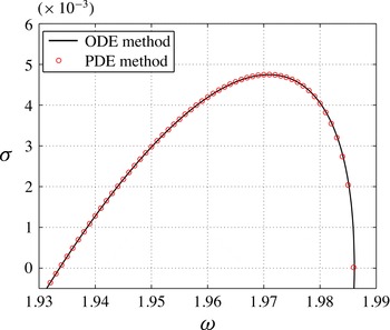
problem. The ordinary differential equation (ODE) eigenvalue problem with the present boundary conditions has been solved by a shooting iterative method to machine numerical accuracy. These accurate growth rates are shown in figure 1 (the solid line). Also shown in figure 1 are the presently computed results of
 ${\it\sigma}$
of the least stable mode with
 $m=0$
in the range of swirl ratios between
 ${\it\omega}=1.932$
and
 ${\it\omega}=1.986$
(the open circles). In this range of swirl ratio,
 ${\it\sigma}$
of the least stable mode is real. It is evident that the present computations using a mesh size of
 $600\times 250$
give accurate results of the growth rates for
 $m=0$
.
A comparison of the growth rates
 ${\it\sigma}$
as a function of
 ${\it\omega}$
for the inviscid axisymmetric perturbation mode with
 $m=0$
and the case of
 $L=6$
. The present computations are presented by the open circles and the accurate ODE results by the solid line.

In order to validate the computed results, we also conducted a thorough mesh convergence study by using various sizes of meshes for the modes
 $m=0,1,2$
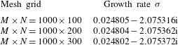
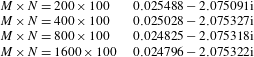
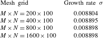
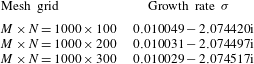
in both the inviscid and viscous flow cases. Tables 1 and 2 compare for various meshes the computed results of
 ${\it\sigma}$
of the most unstable linear mode of the solid-body rotation flow with
 $m=1$
for a representative inviscid flow case with
 ${\it\omega}=2.1$
and
 $L=6$
. From table 1 we find that the computed
 ${\it\sigma}$
change by only
 ${\sim}10^{-6}$
when the mesh radial resolution is increased from
 $N=100$
to
 $N=300$
with a fixed
 $M=1000$
. This demonstrates that a mesh with
 $N=100$
in the radial direction is sufficient for an accurate computation of
 ${\it\sigma}$
. From table 2 we find that the computed
 ${\it\sigma}$
change by
 ${\sim}6\times 10^{-4}$
when the mesh axial resolution is increased from
 $M=200$
to
 $M=1600$
with a fixed
 $N=100$
(approximately
 $2.4\,\%$
inaccuracy in computing the real part of
 ${\it\sigma}$
and less than
 $0.1\,\%$
inaccuracy in computing the imaginary part of
 ${\it\sigma}$
). This demonstrates that a mesh of
 $M=800\times N=100$
is sufficient for an accurate computation of
 ${\it\sigma}$
of the various
 $m=1$
modes in the inviscid flow case. Similarly, we find that a mesh of
 $M=800\times N=100$
is also sufficient for an accurate computation of
 ${\it\sigma}$
of the various
 $m=0$
and
 $m=2$
modes in the inviscid flow case.
Influence of the mesh refinement in radial direction on the computed growth rate of the most unstable linear mode with
 $m=1$
for a representative inviscid flow with
 ${\it\omega}=2.1$
and
 $L=6$
.

Influence of the mesh refinement in axial direction on the computed growth rate of the most unstable linear mode with
 $m=1$
for a representative inviscid flow with
 ${\it\omega}=2.1$
and
 $L=6$
.

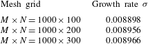
Influence of the mesh refinement in radial direction on the computed
 ${\it\sigma}$
of the most unstable linear mode with
 $m=0$
,
 $Re=1000$
at
 ${\it\omega}=2.15$
and
 $L=6$
.

Influence of the mesh refinement in axial direction on the computed
 ${\it\sigma}$
of the most unstable linear mode with
 $m=0$
,
 $Re=1000$
at
 ${\it\omega}=2.15$
and
 $L=6$
.

Tables 3 and 4 compare for various meshes the computed results of
 ${\it\sigma}$
of the most unstable linear mode with
 $m=0$
for a representative viscous flow case with
 ${\it\omega}=2.15$
,
 $Re=1000$
and
 $L=6$
. These tables demonstrate that a mesh of
 $M=800\times N=100$
is again sufficient for an accurate computation of
 ${\it\sigma}$
of the
 $m=0$
modes in the viscous flow case.
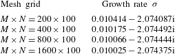
Similarly, tables 5 and 6 compare for various meshes the computed results of the growth rate of the most unstable linear mode with
 $m=1$
for a representative viscous flow case with
 ${\it\omega}=2.1$
,
 $Re=1000$
and
 $L=6$
. These tables demonstrate again that a mesh of
 $M=800\times N=100$
is sufficient for an accurate computation (within 1 % or less) of
 ${\it\sigma}$
of the various
 $m=1$
modes in the viscous flow case. Comparing the results for same
 ${\it\omega}=2.1$
from the inviscid flow case in table 2 and from the
 $Re=1000$
case in table 6, we find that the real part of
 ${\it\sigma}$
decreases with the addition of the viscous effect while the imaginary part stays nearly the same. We later demonstrate in §§ 5 and 6 that the viscous effect is rather passive and nearly the same for all
 ${\it\omega}$
in the range of studied swirl ratios. We also find (not shown) that a mesh of
 $M=800\times N=100$
is sufficient for an accurate computation of
 ${\it\sigma}$
of the various
 $m=2$
modes in the various viscous flow cases.
Influence of the mesh refinement in radial direction on the computed growth rate of the most unstable linear mode with
 $m=1$
, at
 ${\it\omega}=2.1$
,
 $Re=1000$
and
 $L=6$
.

Influence of the mesh refinement in axial direction on the computed growth rate of the most unstable linear mode with
 $m=1$
at
 ${\it\omega}=2.1$
,
 $Re=1000$
and
 $L=6$
.

4 Inviscid flow perturbation modes on a solid-body rotation flow
In this section we present the results of growth rates and shapes of modes for
 $m=0,1,2$
.
4.1 The
 $m=0$
modes

We first consider the axisymmetric (
 $m=0$
) perturbation modes. A similar linear stability problem was first studied analytically by Wang & Rusak (Reference Wang and Rusak1996a
). The present stability equations (2.11a–d
) result in a system of linear partial differential equations for the solution of the eigenvalue
 ${\it\sigma}$
. The problem has a continuum of solutions of perturbation modes that turn in sequence from being asymptotically stable to unstable as
 ${\it\omega}$
is increased above the first critical swirl
 ${\it\omega}_{0,1}$
, where
 ${\it\omega}_{0,1}=\sqrt{{\it\omega}_{B}^{2}+{\rm\pi}^{2}/(4L^{2})}$
(here
 ${\it\omega}_{B}=1.9159$
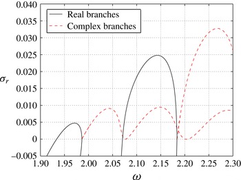
is Benjamin’s (Reference Benjamin1962) special swirl). The growth rates
 ${\it\sigma}_{r}$
(the real part of
 ${\it\sigma}$
) as a function of the swirl ratio
 ${\it\omega}$
of the various
 $m=0$
perturbation modes on the solid-body rotation flow in a pipe with
 $L=6$
are shown in figure 2.
The growth rates
 ${\it\sigma}_{r}$
(the real part of
 ${\it\sigma}$
) as a function of the swirl ratio
 ${\it\omega}$
of the various inviscid axisymmetric (
 $m=0$
) perturbation modes on a solid-body rotation flow in a pipe with
 $L=6$
.

It is found that that all modes have real values of
 ${\it\sigma}$
that are negative and real shape functions when
 $0<{\it\omega}<{\it\omega}_{0,1}=1.9337$
, i.e. all the
 $m=0$
modes are asymptotically stable when the swirl ratio is below the first
 $m=0$
critical swirl. The
 ${\it\sigma}$
of the least stable mode is real and changes from negative to positive, and the flow becomes unstable as
 ${\it\omega}$
is increased from below the first critical swirl
 ${\it\omega}_{0,1}=1.9337$
to above it. The growth rate
 ${\it\sigma}_{r}$
of the
 $k=1$
mode increases in the range
 ${\it\omega}_{0,1}=1.9337<{\it\omega}<1.971$
, reaches a maximum value of
 $0.00475$
at
 ${\it\omega}=1.971$
and then decreases in the range
 $1.971<{\it\omega}<{\it\omega}_{0,2}$
, where
 ${\it\omega}_{0,2}=\sqrt{{\it\omega}_{B}^{2}+{\rm\pi}^{2}/L^{2}}=1.9862$
is the second critical swirl. This swirl level is also a fold point of
 ${\it\sigma}_{r}$
of the first least stable mode.
The growth rate
 ${\it\sigma}_{r}$
of the second (
 $k=2$
) mode changes from negative to zero as
 ${\it\omega}$
increases to the second critical swirl
 ${\it\omega}_{0,2}=1.9862$
. We note that the real growth rates of the two least stable modes merge to form the first fold point at
 ${\it\omega}_{0,2}=1.9862$
where for both modes
 ${\it\sigma}_{r}=0$
. All the other perturbation modes have real negative
 ${\it\sigma}$
and real shape functions and are asymptotically stable in the range
 ${\it\omega}_{0,1}<{\it\omega}<{\it\omega}_{0,2}$
. The two least stable modes combine together at
 ${\it\omega}_{0,2}=1.9862$
to form a pair of modes with complex-conjugate values of
 ${\it\sigma}$
and mode shape functions in the range
 ${\it\omega}>{\it\omega}_{0,2}$
. Only the real part
 ${\it\sigma}_{r}$
of these two modes is shown in figure 2; it increases in the range
 ${\it\omega}_{0,2}=1.9852<{\it\omega}<2.045$
, reaches a maximum of
 $0.0095$
at
 ${\it\omega}=2.045$
and then deceases in the range
 $2.045<{\it\omega}<{\it\omega}_{0,3}$
, where
 ${\it\omega}_{0,3}=\sqrt{{\it\omega}_{B}^{2}+9{\rm\pi}^{2}/(4L^{2})}=2.0706$
. These two complex-conjugate modes have an oscillatory behaviour of
 ${\it\sigma}_{r}$
as
 ${\it\omega}$
increases above
 ${\it\omega}_{0,3}=2.0706$
.
The
 ${\it\sigma}_{r}$
of the third (
 $k=3$
) least stable mode changes from negative to positive as
 ${\it\omega}$
increases from below the third critical swirl
 ${\it\omega}_{0,3}=2.0706$
to above it. The growth rate and shape functions of this mode are real and become dominant in the range
 ${\it\omega}_{0,3}<{\it\omega}<{\it\omega}_{0,4}$
, where
 ${\it\omega}_{0,4}=\sqrt{{\it\omega}_{B}^{2}+4{\rm\pi}^{2}/L^{2}}=2.1834$
. Additional
 $m=0$
perturbation modes with either real or complex values of the growth rates and shape functions appear in sequence as
 ${\it\omega}$
increases above an additional critical swirl
 ${\it\omega}_{0,n}=\sqrt{{\it\omega}_{B}^{2}+n^{2}{\rm\pi}^{2}/(4L^{2})}$
(here
 $n$
is a positive integer). By using the perturbation theory of the linear operators (see Wang Reference Wang2008), it can be shown that the critical swirl levels with even values of
 $n$
are also fold points of the
 ${\it\sigma}_{r}$
plots and complex-conjugate modes appear at these fold swirl levels. Also, the critical swirl levels with odd values of
 $n$
are points of exchange of stability of a mode with real
 ${\it\sigma}$
and shape functions. The dominant unstable
 $m=0$
perturbation at each swirl ratio is the perturbation mode with the greatest value of
 ${\it\sigma}_{r}$
at that swirl level.
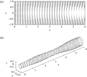
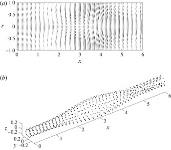
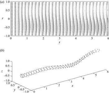
Figure 3 shows a representative example of the solution of the most unstable
 $m=0$
(axisymmetric) mode shape functions at
 ${\it\omega}=2.13$
(between
 ${\it\omega}_{0,3}$
and
 ${\it\omega}_{0,4}$
) in a pipe with
 $L=6$
for which
 ${\it\sigma}=0.025$
(on solution branch
 $k=3$
of
 $m=0$
case). Figure 3(a) presents the computed planar projected velocity vector,
 $(1+{\it\epsilon}\mathscr{W},{\it\epsilon}\mathscr{U})$
, of the mode in the flow domain; here
 $\mathscr{W}$
and
 $\mathscr{U}$
are real and
 ${\it\epsilon}$
is the perturbation’s amplitude such that there is a near stagnation point at the pipe outlet. Figure 3(b) describes a snapshot of the streaklines of the mode consisting of particles released at the pipe inlet (
 $x=0$
) on a circle with
 $r=0.15$
. It can be seen that the mode describes an axisymmetric axial growing wave with a wavelength of approximately
 $3.6$
and an amplitude that grows in
 $x$
. Similar figures can be given for all other computed
 $m=0$
modes.
The shape functions of the dominant inviscid unstable
 $m=0$
mode at
 ${\it\omega}=2.13$
: (a) planar projected velocity vector field; (b) the streaklines of the mode consisting of particles released at the pipe inlet (
 $x=0$
) on a circle with
 $r=0.15$
.

4.2 The
$m=1$
modes

In parallel to the
 $m=0$
modes, the stability problem with
 $m=1$
also has a continuum of solutions of spiral perturbation modes that are studied in this paper for the first time. The growth rates
 ${\it\sigma}_{r}$
(the real part of
 ${\it\sigma}$
) and frequency
 ${\it\sigma}_{i}$
(the imaginary part of
 ${\it\sigma}$
) as a function of the swirl ratio
 ${\it\omega}$
of the various inviscid
 $m=1$
perturbation modes on the solid-body rotation flow in a pipe with
 $L=6$
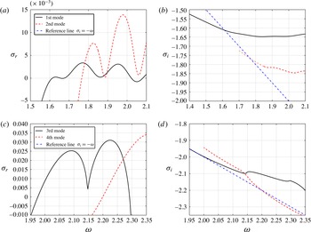
are shown in figure 4. Each of the different modes is characterized by a continuous solution as a function of
 ${\it\omega}$
with a similar axial wavelength of the shape functions that increases with the mode number
 $k$
. The modes are numbered
 $k=1,k=2,$
and so on. Figure 4(a) describes
 ${\it\sigma}_{r}$
of the modes
 $k=1$
and
 $k=2$
in the range
 $1.5\leqslant {\it\omega}\leqslant 2.1$
and figure 4(b) describes the corresponding
 ${\it\sigma}_{i}$
of these modes. Figure 4(c) describes
 ${\it\sigma}_{r}$
of the modes
 $k=3$
and
 $k=4$
in the range
 $1.95\leqslant {\it\omega}\leqslant 2.35$
and figure 4(d) describes the corresponding
 ${\it\sigma}_{i}$
of these modes.
The growth rates
 ${\it\sigma}$
as a function of the swirl ratio
 ${\it\omega}$
of the various
 $m=1$
spiral perturbation modes on a solid-body rotation flow in a pipe with
 $L=6$
; (a)
 ${\it\sigma}_{r}$
of modes
 $k=1$
and
 $k=2$
, (b)
 ${\it\sigma}_{i}$
of modes
 $k=1$
and
 $k=2$
, (c)
 ${\it\sigma}_{r}$
of modes
 $k=3$
and
 $k=4$
, (d)
 ${\it\sigma}_{i}$
of modes
 $k=3$
and
 $k=4$
.

It is found that each one of these complex modes turns in sequence from being asymptotically stable to unstable as
 ${\it\omega}$
is increased. Mode
 $k=1$
changes its stability at the swirl level
 ${\it\omega}_{1,1}=1.613$
and reaches a local maximum positive value of
 ${\it\sigma}_{r}=0.000253$
at
 ${\it\omega}=1.629$
(figure 4
a). Then
 ${\it\sigma}_{r}$
of this mode continues with oscillations as
 ${\it\omega}$
is further increased and has maximum points of
 ${\it\sigma}_{r}=0.00335$
at
 ${\it\omega}=1.771$
, of
 ${\it\sigma}_{r}=0.00308$
at
 ${\it\omega}=1.954$
and so on. Similarly, mode
 $k=2$
changes its stability at the swirl level
 ${\it\omega}_{1,2}=1.766$
and reaches a maximum of
 ${\it\sigma}_{r}=0.00765$
at
 ${\it\omega}=1.826$
(figure 4
a). The
 ${\it\sigma}_{r}$
of this mode continues with oscillations as
 ${\it\omega}$
is further increased with a maximum point of
 ${\it\sigma}_{r}=0.0139$
at
 ${\it\omega}=1.978$
. The higher-order modes with
 $k=3$
and
 $k=4$
exhibit a similar behaviour (figure 4
c). The mode
 $k=3$
becomes unstable at swirl level
 ${\it\omega}_{1,3}=1.976$
and the mode
 $k=4$
becomes unstable at swirl level
 ${\it\omega}_{1,4}=2.199$
. We note that each mode reaches a maximum of
 ${\it\sigma}_{r}$
that increases with the mode number
 $k$
. This mode becomes the dominant unstable mode in the range of swirl around its maximum of
 ${\it\sigma}_{r}$
.
In contrast to the
 $m=0$
results, the growth rates
 ${\it\sigma}$
are all complex in the
 $m=1$
case since the equations contain
 $\text{i}{\it\omega}$
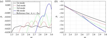
terms which reflect the rotation of the azimuthal wave. The imaginary part
 ${\it\sigma}_{i}$
of the modes describes the rate of rotation of the mode around the pipe centreline. For all modes
 ${\it\sigma}_{i}$
is negative, indicating a rotation of the mode in the direction of the base flow rotation. For this case with
 $m=1$
the values of
 ${\it\sigma}_{i}$
as a function of
 ${\it\omega}$
are close to
 $-{\it\omega}$
, i.e. the rate of rotation of the mode is close to the negative rate of rotation of the base flow (see reference dash-dot blue line
 ${\it\sigma}_{i}=-{\it\omega}$
in figures 4
b and 4
d). When
 $|{\it\sigma}_{i}|>{\it\omega}$
, the mode rotates around the centreline with an angular speed that is greater than that of the base flow and, when
 $|{\it\sigma}_{i}|<{\it\omega}$
, the mode rotates around the centreline with an angular speed that is less than that of the base flow. For example, mode
 $k=1$
has a faster rate of rotation than the base flow when
 ${\it\omega}<1.613$
and has a slower rate of rotation than the base flow when
 ${\it\omega}>1.613$
. Similarly, mode
 $k=2$
has a faster rate of rotation than the base flow when
 ${\it\omega}<1.766$
and has a slower rate of rotation than the base flow when
 ${\it\omega}>1.766$
. We find that for each of the modes
 $k=1$
through
 $k=4$
with
 $m=1$
, the value of
 ${\it\sigma}+\text{i}{\it\omega}=0$
at the swirl levels
 ${\it\omega}_{1,k}$
where
 ${\it\sigma}_{r}=0$
.
We note that
 ${\it\omega}_{1,1}$
is less than
 ${\it\omega}_{0,1}$
; i.e. there exists a range of swirl
 ${\it\omega}_{1,1}\leqslant {\it\omega}\leqslant {\it\omega}_{0,1}$
where only
 $m=1$
unstable growing perturbations appear on the solid-body rotation flow and before the appearance of unstable axisymmetric
 $m=0$
modes. Additional comparison between the axisymmetric and the
 $m=1$
unstable modes is shown in the next section.
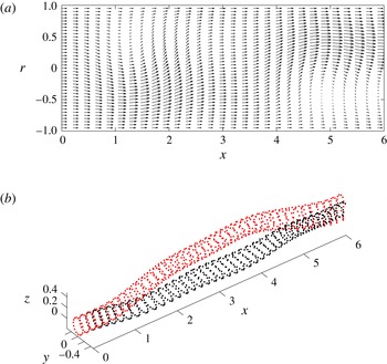
Figure 5 shows a representative example of the solution of the dominant unstable
 $m=1$
rotating spiral mode shape functions at
 ${\it\omega}=2$
in a pipe with
 $L=6$
for which
 ${\it\sigma}=0.0127-\text{i}1.840$
(on the solution branch of
 $k=2$
mode with
 $m=1$
). Figure 5(a) presents the computed planar projected velocity vector,
 $(1+{\it\epsilon}\text{Re}(\mathscr{W}),{\it\epsilon}\text{Re}(\mathscr{U}))$
, of this mode in the flow domain; here
 ${\it\epsilon}$
is the perturbation’s amplitude such that there are two stagnation points inside the domain and near the pipe outlet. Figure 5(b) describes two snapshots of streaklines of the mode at two non-dimensional times that are
 ${\rm\Delta}t={\rm\pi}/(2|{\it\sigma}_{i}|)=0.854$
apart. Both streaklines consist of particles released at the pipe inlet (
 $x=0$
) on a circle with
 $r=0.15$
. It can be seen that the mode describes a rotating spiral perturbation in the direction of flow rotation. Figure 5(a) qualitatively resembles the velocity field that is shown in figures 1(a) and 1(b) in Spall & Gatski (Reference Spall and Gatski1991) at the initial stage of perturbation’s growth to a spiral type of breakdown. Similar figures can be given for all other computed
 $m=1$
modes.
The shape functions of the dominant inviscid unstable
 $m=1$
mode at
 ${\it\omega}=2$
: (a) planar projected velocity vector field; (b) two streaklines of the spiral mode at times
 ${\rm\Delta}t={\rm\pi}/(2|{\it\sigma}_{i}|)=0.854$
apart that consist of particles released at the pipe inlet (
 $x=0$
) on a circle with
 $r=0.15$
.

4.3 The
$m=2$
modes

The stability problem with
 $m=2$
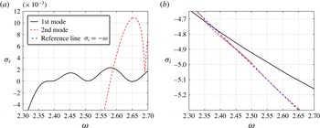
has a continuum of solutions of double-spiral perturbation modes. For this case the growth rates
 ${\it\sigma}$
are all complex,
 ${\it\sigma}={\it\sigma}_{r}+\text{i}{\it\sigma}_{i}$
. The growth rate
 ${\it\sigma}_{r}$
and frequency
 ${\it\sigma}_{i}$
as a function of the swirl ratio
 ${\it\omega}$
of the various
 $m=2$
perturbation modes on the solid-body rotation flow in a pipe with
 $L=6$
are shown in figure 6. Again, each of the different modes is characterized by a continuous solution as a function of
 ${\it\omega}$
with a similar axial wavelength of the shape functions that increases with the mode number. Figure 6(a) describes
 ${\it\sigma}_{r}$
of the modes
 $k=1$
and
 $k=2$
in the range
 $2.34\leqslant {\it\omega}\leqslant 2.5$
and figure 6(b) describes the corresponding
 ${\it\sigma}_{i}$
of these modes. Figure 6(a) shows that mode
 $k=1$
changes stability at
 ${\it\omega}_{2,1}=2.377$
, reaches a maximum value of
 ${\it\sigma}_{r}=2.04\times 10^{-5}$
at
 ${\it\omega}=2.383$
and then
 ${\it\sigma}_{r}$
of this mode continues with oscillations as
 ${\it\omega}$
is further increased. Similarly, mode
 $k=2$
changes stability at the critical swirl
 ${\it\omega}_{2,2}=2.387$
, reaches a maximum of
 ${\it\sigma}_{r}=0.00147$
at
 ${\it\omega}=2.454$
and
 ${\it\sigma}_{r}$
of this mode also continues with oscillations as
 ${\it\omega}$
is further increased. Figure 6(b) shows that the frequency
 ${\it\sigma}_{i}$
of these modes is around
 $2{\it\omega}$
. Additional modes become unstable in sequence as
 ${\it\omega}$
is further increased.
The growth rates
 ${\it\sigma}$
as a function of the swirl ratio
 ${\it\omega}$
of the various
 $m=2$
double-spiral perturbation modes on a solid-body rotation flow in a pipe with
 $L=6$
; (a)
 ${\it\sigma}_{r}$
of modes
 $k=1$
and
 $k=2$
, (b)
 ${\it\sigma}_{i}$
of modes
 $k=1$
and
 $k=2$
.

Figure 7 shows a representative example of the solution of the dominant unstable
 $m=2$
double-spiral mode shape functions at
 ${\it\omega}=2.454$
in a pipe with
 $L=6$
for which
 ${\it\sigma}=0.00147-\text{i}4.86$
(on solution branch
 $k=2$
of
 $m=2$
case). Figure 7(a) presents the computed planar projected velocity vector,
 $(1+{\it\epsilon}\text{Re}(\mathscr{W}),{\it\epsilon}\text{Re}(\mathscr{U}))$
, of this mode in the flow domain; here
 ${\it\epsilon}$
is the perturbation’s amplitude such that there is a reversed flow at the middle of the pipe. Figure 7(b) describes a snapshot of streakline of the mode that consists of particles released at the pipe inlet (
 $x=0$
) on a circle with
 $r=0.15$
. It can be seen that the mode describes a rotating double-spiral perturbation in the direction of flow rotation with almost twice the base flow rate of rotation. Similar figures can be given for all other computed
 $m=2$
modes.
The shape functions of the dominant inviscid unstable
 $m=2$
mode at
 ${\it\omega}=2.454$
: (a) planar projected velocity vector field; (b) one streakline of the double-spiral mode that consists of particles released at the pipe inlet (
 $x=0$
) on a circle with
 $r=0.15$
.

4.4 The comparison between the growth rates
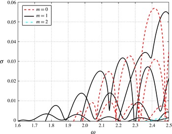
The growth rates computed for the various perturbation modes at
 $m=0$
,
 $m=1$
and
 $m=2$
are compared in figure 8 in the range of swirl
 $1.6\leqslant {\it\omega}\leqslant 2.5$
. It is found that all perturbation modes are asymptotically stable when
 ${\it\omega}<{\it\omega}_{1,1}=1.613$
. The first four of the
 $m=1$
perturbation modes become unstable in sequence when
 ${\it\omega}_{1,1}=1.613\leqslant {\it\omega}\leqslant {\it\omega}_{0,1}=1.9337$
. Although axisymmetric perturbation modes appear in sequence as well when
 ${\it\omega}>{\it\omega}_{0,1}$
, their growth rates are less than those of the second and third
 $m=1$
spiral modes when
 ${\it\omega}_{0,1}=1.9337\leqslant {\it\omega}\leqslant 2.118$
. These
 $m=1$
spiral modes are the fastest growing perturbations in this range of swirl. An example of such a dominant unstable spiral mode at
 ${\it\omega}=2$
is shown in figure 5. The third axisymmetric
 $m=0$
mode has the greatest growth rate in the range of swirl
 $2.118<{\it\omega}<2.170$
and is the dominant unstable mode in those range. An example of such a dominant unstable axisymmetric mode at
 ${\it\omega}=2.13$
is shown in figure 3. Similarly, higher-order
 $m=1$
and
 $m=0$
perturbation modes become the dominant unstable modes in sequence and switch roles in certain ranges of swirl as the swirl ratio
 ${\it\omega}$
is further increased. We note that the
 $m=2$
double-spiral unstable modes appear only when
 ${\it\omega}_{2,1}=2.397<{\it\omega}<2.5$
but their growth rates
 ${\it\sigma}_{r}$
are much smaller than those of the axisymmetric and
 $m=1$
spiral modes and they are insignificant in terms of the dynamics of the flow in this range of swirl.
A comparison between the growth rates of the various
 $m=0,1,2$
inviscid flow instability modes.

The comparison between the various computed perturbation modes shows that in the inviscid flow case the solid-body rotation flow undergoes a complicated dynamical process as the swirl ratio increases. When
 ${\it\omega}<1.613$
the flow is asymptotically stable and any axisymmetric or three-dimensional perturbation decays in time and the flow returns to a columnar state.
In the range of swirl
 ${\it\omega}_{1,1}=1.613<{\it\omega}<{\it\omega}_{0,1}=1.9337$
small perturbations grow as spiral waves. Moreover, Rusak & Wang (Reference Rusak and Wang2014) recently revealed that the swirl ratio
 ${\it\omega}_{0,1}$
has an important role in the global dynamics of perturbed inviscid and axisymmetric flows. Only when
 ${\it\omega}>{\it\omega}_{0,1}$
there exist two strong axisymmetric attractors of the flow dynamics; the first is a vortex breakdown state with a near-stagnation zone around the pipe centreline and the second is a wall-separation state with a quasi-stagnation zone attached to the pipe wall. Such flow attractors do not exist when
 $0\leqslant {\it\omega}<{\it\omega}_{0,1}$
. Therefore, these states are not global attractors of the flow dynamics as the specific unstable spiral
 $m=1$
modes grow in the range
 ${\it\omega}_{1,1}=1.613<{\it\omega}<{\it\omega}_{0,1}=1.9337$
. The evolution of the three-dimensional perturbations in this swirl range is yet unknown and may be studied by further analysis using numerical simulations.
In the range of swirl
 ${\it\omega}>{\it\omega}_{0,1}$
any initial sufficiently small perturbation evolves in the beginning according to the most unstable perturbation mode found in figure 8. However, the long-term dynamics of the perturbation growth, either spiral or axisymmetric, is not yet clear. It may either grow according to the linear theory for a long time and be attracted to one of the axisymmetric global attractors mentioned above (as shown theoretically and demonstrated numerically by Rusak & Wang (Reference Rusak and Wang2014)) or it may evolve into a complicated three-dimensional unsteady state that may include a spiral breakdown state. The current inviscid flow linear stability analysis reveals the initial evolution of perturbations and further analysis using numerical simulations is needed.
5 Viscous flow perturbation modes on a solid-body rotation flow
In this section we present the computed perturbation modes on a solid-body rotation flow at
 $Re=500$
and
 $Re=1000$
. We consider a typical non-dimensional pipe length
 $L=6$
.
5.1 The
$m=0$
modes

We first consider the axisymmetric (
 $m=0$
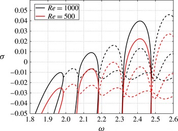
) perturbation modes. The growth rates
 ${\it\sigma}_{r}$
as a function of the swirl ratio
 ${\it\omega}$
of the various
 $m=0$
modes are shown in figure 9 for
 $Re=500$
(the red line) and for
 $Re=1000$
(the black line).
It is found at
 $Re=500$
that all the modes have only real negative values of
 ${\it\sigma}$
when
 ${\it\omega}<1.985$
. At
 ${\it\omega}=1.985$
the modes
 $k=1$
and
 $k=2$
join together to form a fold point of their
 ${\it\sigma}_{r}$
curve. Then, these modes yield two branches of complex-conjugate growth rates with the same
 ${\it\sigma}_{r}<0$
that oscillates with
 ${\it\omega}$
when
 ${\it\omega}>1.985$
. The modes
 $k=3$
and
 $k=4$
exhibit a similar behaviour. They also have real negative growth rates when
 ${\it\omega}<2.18$
and form a fold point at
 ${\it\omega}=2.18$
from which two additional branches of complex-conjugate growth rates appear with same
 ${\it\sigma}_{r}<0$
that also oscillates with
 ${\it\omega}$
when
 ${\it\omega}>2.18$
. The mode
 $k=5$
also has real values of
 ${\it\sigma}_{r}$
when
 ${\it\omega}<2.475$
. This mode is the first mode that shows a change of the growth rate from negative to positive values at
 ${\it\omega}_{0,1}=2.3386$
. The swirl ratio
 ${\it\omega}_{0,1}=2.3386$
is the first critical swirl of the
 $m=0$
modes at
 $Re=500$
. All the
 $m=0$
modes are asymptotically stable for
 ${\it\omega}<2.3386$
at
 $Re=500$
. The growth rate of the
 $k=5$
mode is positive and this mode is unstable in the range of
 $2.3386<{\it\omega}<2.47$
. The swirl ratio
 ${\it\omega}_{0,2}=2.47$
is the second critical swirl of the
 $m=0$
modes at
 $Re=500$
at which this mode becomes asymptotically stable again. With further increase of
 ${\it\omega}$
, the modes
 $k=5$
and
 $k=6$
join together to form a fold point of their
 ${\it\sigma}_{r}$
curve at
 ${\it\omega}=2.475$
from which two additional branches of complex-conjugate growth rates appear. The
 ${\it\sigma}_{r}$
of these branches changes from negative to positive values at the third critical swirl ratio
 ${\it\omega}_{0,3}=2.495$
and then change back to negative values at the next critical swirl ratio
 ${\it\omega}_{0,4}=2.637$
. Additional higher-order instability modes appear in sequence as
 ${\it\omega}$
is further increased.
The case with
 $Re=1000$
exhibits a similar behaviour (see figure 9) but with reduced values of the critical swirl ratios where
 ${\it\sigma}_{r}$
changes its sign. In the
 $Re=1000$
case, the mode
 $k=3$
is the first to become unstable at
 ${\it\omega}_{0,1}=2.09$
and then becomes asymptotically stable at
 ${\it\omega}_{0,2}=2.177$
. The modes
 $k=3$
and
 $k=4$
join together at
 ${\it\omega}=2.18$
to form two complex-conjugate modes that become unstable at
 ${\it\omega}_{0,3}=2.205$
and then stabilize at
 ${\it\omega}_{0,4}=2.311$
. Again, additional higher-order instability modes appear in sequence as
 ${\it\omega}$
is further increased.
The comparison between the various
 ${\it\sigma}_{r}$
curves of the
 $m=0$
modes at
 $Re=500$
and
 $Re=1000$
shows that the values of
 ${\it\sigma}_{r}$
for each mode
 $k$
increase by a nearly constant value in the range of
 ${\it\omega}$
studied as
 $Re$
is increased. The effect of viscosity on the
 $m=0$
modes is passive. This is confirmed by the perturbation’s kinetic energy analysis in § 6.
The growth rates
 ${\it\sigma}$
as a function of the swirl ratio
 ${\it\omega}$
of the various axisymmetric (
 $m=0$
) perturbation modes on a solid-body rotation flow in a pipe with
 $L=6$
; the red line is for
 $Re=500$
and the black line is for
 $Re=1000$
.

The shapes of the various
 $m=0$
modes at both
 $Re=500$
and
 $Re=1000$
are similar to their counterparts in the inviscid flow case, shown for example in figure 3 for the
 $k=3$
mode at
 ${\it\omega}=2.13$
.
5.2 The
$m=1$
modes

Similar to the inviscid flow case, the viscous flow stability problem with
 $m=1$
also has a continuum of solutions of spiral perturbation modes, all of them with a complex value of
 ${\it\sigma}={\it\sigma}_{r}+i{\it\sigma}_{i}$
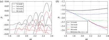
. The growth rates
 ${\it\sigma}_{r}$
and frequency
 ${\it\sigma}_{i}$
as a function of the swirl ratio
 ${\it\omega}$
of the various
 $m=1$
perturbation modes on the solid-body rotation flow in a pipe of length
 $L=6$
are shown in figure 10. Each of the
 $m=1$
modes is characterized by a continuous solution as a function of
 ${\it\omega}$
with same axial wavelength of the shape functions that increases with the mode number
 $k$
where
 $k=1,2,3,4$
and so on.
The growth rates
 ${\it\sigma}$
as a function of the swirl ratio
 ${\it\omega}$
of the various
 $m=1$
spiral perturbation modes on a solid-body rotation flow in a pipe with
 $L=6$
; (a)
 ${\it\sigma}_{r}$
for
 $Re=500$
(red line) and
 $Re=1000$
(black line), (b)
 ${\it\sigma}_{i}$
for
 $Re=1000$
.

Figure 10(a) describes the curves of
 ${\it\sigma}_{r}$
as a function pf
 ${\it\omega}$
of the modes
 $k=1$
through
 $k=4$
in the range
 $1.6\leqslant {\it\omega}\leqslant 2.6$
for
 $Re=500$
(the red lines) and
 $Re=1000$
(the black lines). For the case
 $Re=500$
, we find that the
 $k=1$
mode has an oscillatory variation of
 ${\it\sigma}_{r}<0$
and is asymptotically stable in the entire range of swirl studied. Similarly, the
 $k=2$
mode also has an oscillatory change of
 ${\it\sigma}_{r}$
and is negative in the range of swirl studied. The
 $k=3$
mode is the first to become unstable at the swirl ratio
 ${\it\omega}_{1,1}=2.206$
; i.e. all the
 $m=1$
perturbation modes are asymptotically stable when
 ${\it\omega}<{\it\omega}_{1,1}<2.206$
. The
 $k=3$
mode is unstable in the range
 $2.206<{\it\omega}<2.244$
and reaches a maximum value of
 ${\it\sigma}_{r}=0.0012$
at
 ${\it\omega}=2.225$
. The swirl ratio
 ${\it\omega}_{1,2}=2.244$
is the second critical swirl. The mode
 $k=3$
becomes asymptotically stable when
 ${\it\omega}>2.244$
with
 ${\it\sigma}_{r}<0$
that oscillates as
 ${\it\omega}$
is further increased. The
 $k=4$
mode changes its stability at the critical swirl
 ${\it\omega}_{1,3}=2.401$
, reaches a maximum values of
 ${\it\sigma}_{r}=0.0182$
at
 ${\it\omega}=2.483$
and
 ${\it\sigma}_{r}$
of this mode continues to stay positive and exhibits oscillations as
 ${\it\omega}$
is further increased within the specified swirl range. Higher-order critical swirl ratios and instability modes with
 $m=1$
appear in sequence and exhibit a similar behaviour. We note that the maximum of
 ${\it\sigma}_{r}$
of the modes with
 $m=1$
increases with the mode number
 $k$
.
The case with
 $Re=1000$
exhibits a similar behaviour (see figure 10
a) but with reduced values of the critical swirl ratios where
 ${\it\sigma}_{r}$
changes its sign. In the
 $Re=1000$
case, the mode
 $k=2$
is the first to become unstable at
 ${\it\omega}_{1,1}=1.960$
and then becomes asymptotically stable at
 ${\it\omega}_{1,2}=1.998$
. The
 $k=3$
mode becomes unstable at
 ${\it\omega}_{1,3}=2.022$
. Again, additional critical swirl ratios and instability modes appear in sequence as
 ${\it\omega}$
is further increased.
The comparison between the various
 ${\it\sigma}_{r}$
curves of the
 $m=1$
modes at
 $Re=500$
and
 $Re=1000$
shows that the values of
 ${\it\sigma}_{r}$
for each mode
 $k$
increase by a nearly constant value in the range of
 ${\it\omega}$
studied as
 $Re$
is increased. The effect of viscosity on the
 $m=1$
modes is passive and this is also confirmed by the perturbation’s kinetic energy analysis in § 6.
The imaginary part
 ${\it\sigma}_{i}$
of the various modes with
 $m=1$
is shown in figure 10(b) for the case
 $Re=1000$
. Also shown in this figure is the reference line
 ${\it\sigma}_{i}=-{\it\omega}$
(the dash-dot blue line). The value of
 ${\it\sigma}_{i}$
describes the rate of rotation of the mode around the pipe centreline. We find that at the change of stability swirl ratio
 ${\it\omega}_{1,1}=1.960$
of the
 $k=2$
mode
 ${\it\sigma}_{i}$
is above the reference line, i.e.
 $-{\it\omega}_{1,1}<{\it\sigma}_{i}<0$
for
 ${\it\omega}>{\it\omega}_{1,1}$
. This means that the
 $k=2$
mode with
 $m=1$
rotates around the centreline at a clearly slower rate than the base flow. This is a direct result of the viscous effects.
Figure 11 shows a representative example of the solution of the dominant unstable
 $m=1$
rotating spiral mode shape functions at
 ${\it\omega}=2.48,Re=500$
in a pipe with
 $L=6$
for which
 ${\it\sigma}=0.0181-i2.438$
(on the solution branch of
 $k=4$
mode with
 $m=1$
). Figure 11(a) presents the computed planar projected velocity vector,
 $(1+{\it\epsilon}\text{Re}(\mathscr{W}),{\it\epsilon}\text{Re}(\mathscr{U}))$
, of this mode in the flow domain. Figure 11(b) describes a snapshot of streaklines of the mode. The streakline consists of particles released at the pipe inlet (
 $x=0$
) on a circle with
 $r=0.15$
. It can be seen that the mode describes a rotating spiral perturbation that is similar to the inviscid mode shape shown in figure 5. Also, figure 11(a) qualitatively resembles the velocity field that is shown in figures 1(a) and 1(b) in Spall & Gatski (Reference Spall and Gatski1991) at the initial stage of perturbation’s growth to a spiral type of breakdown.
The shape functions of the dominant unstable
 $m=1$
mode at
 ${\it\omega}=2.48$
: (a) planar projected velocity vector field; (b) the streaklines of the spiral mode that consist of particles released at the pipe inlet (
 $x=0$
) on a circle with
 $r=0.15$
.

5.3 The
$m=2$
modes

The viscous flow stability problem with
 $m=2$
has a continuum of solutions of double-spiral perturbation modes with complex values of
 ${\it\sigma}={\it\sigma}_{r}+i{\it\sigma}_{i}$
and mode shapes. The curves of growth rate
 ${\it\sigma}_{r}$
and the frequency
 ${\it\sigma}_{i}$
as a function of the swirl ratio
 ${\it\omega}$
in the range
 $2.3\leqslant {\it\omega}\leqslant 3$
of the various
 $m=2$
perturbation modes on the solid-body rotation flow in a pipe with
 $L=6$
at
 $Re=1000$
are shown in figure 12. Again, each of the
 $k=1$
through
 $k=4$
modes is characterized by a continuous solution as a function of
 ${\it\omega}$
with the same axial wavelength of the shape function that decreases with the mode number
 $k$
.
The growth rates
 ${\it\sigma}$
as a function of the swirl ratio
 ${\it\omega}$
of the various
 $m=2$
spiral perturbation modes on a solid-body rotation flow in a pipe with
 $Re=1000$
and
 $L=6$
; (a)
 ${\it\sigma}_{r}$
as a function of
 ${\it\omega}$
, (b)
 ${\it\sigma}_{i}$
as a function of
 ${\it\omega}$
.

Figure 12(a) describes
 ${\it\sigma}_{r}$
of the modes
 $k=1$
through
 $k=4$
with
 $m=2$
. It is found that modes
 $k=1$
,
 $k=2$
and
 $k=3$
are asymptotically stable (
 ${\it\sigma}_{r}<0$
) in the entire range of swirl studied. The mode
 $k=4$
is the first to become unstable at the critical swirl ratio
 ${\it\omega}_{2,1}=2.9067$
. The
 $k=4$
mode reaches a maximum value of
 ${\it\sigma}_{r}=0.0066$
at
 ${\it\omega}=2.958$
and becomes asymptotically stable when
 ${\it\omega}$
increases above
 ${\it\omega}_{2,2}=2.999$
. The frequency
 ${\it\sigma}_{i}$
of the various modes with
 $m=2$
is shown in figure 12(b). Also shown in this figure is the reference line
 ${\it\sigma}_{i}=-2{\it\omega}$
(the blue dashed line). Within the studied range of swirl, the frequency of the modes
 $k=1$
through
 $k=4$
is close to or slightly less than twice the rate of rotation of the base flow. The shapes of the various
 $m=2$
modes at
 $Re=1000$
are similar to their counterparts in the inviscid flow case, shown for example in figure 7.
We also find that for the case
 $Re=500$
and
 $m=2$
the modes
 $k=1$
through
 $k=4$
appear in sequence and have similar
 ${\it\sigma}_{r}$
curves and mode shapes to those of the
 $Re=1000$
case but remain asymptotically stable (
 ${\it\sigma}_{r}<0$
) in the entire specified swirl range (not shown). The viscous effects stabilize these modes.
5.4 The neutral stability lines of the perturbation modes
We studied the stability of the solid-body rotation flow in a pipe with length
 $L=6$
for a wide range of
 $Re$
from
 $100$
up to
 $2000$
in the range of swirl ratios
 $0<{\it\omega}\leqslant 3$
. For each
 $Re$
we determined the swirl ratios of the
 $m=0$
,
 $m=1$
and
 $m=2$
modes at which
 ${\it\sigma}_{r}=0$
(a neutral mode) appears for the first time as
 ${\it\omega}$
is increased from zero. The neutral stability lines and the stability and instability domains are shown in the
 $Re$
versus
 ${\it\omega}$
plane in figure 13. The light solid lines represent the neutral lines for the
 $m=0$
modes, the heavy solid lines represent the neutral lines for the
 $m=1$
modes and the dotted lines represent the neutral lines for the
 $m=2$
modes. The shaded area is the unstable flow domain.
The neutral stability lines dividing the stable domain (white area) and unstable domain (shaded area) for various perturbation modes with
 $L=6$
, where the light black lines are for the axisymmetric
 $m=0$
modes, the heavy black lines are for the single-spiral
 $m=1$
modes and the dashed lines are for the double-spiral
 $m=2$
modes.

We find from figure 13 that in the case with
 $L=6$
, the single-spiral
 $m=1$
instability modes are the first to appear as swirl
 ${\it\omega}$
is increased at a fixed
 $Re$
in the range
 $481<Re<2000$
. At lower
 $Re$
,
 $214<Re<481$
, the axisymmetric
 $m=0$
instability modes are the first to appear as swirl ratio is increased at a fixed
 $Re$
. The flow is stable for all
 ${\it\omega}<3$
when
 $Re<214$
. The
 $m=2$
instability modes do not affect the first change of flow stability within the studied range of
 $Re$
and
 ${\it\omega}$
. In addition, when
 ${\it\omega}$
is fixed and
 $Re$
changes, the
 $m=1$
modes may appear first as
 $Re$
is increased at certain ranges of
 ${\it\omega}$
, i.e. the ranges
 $0<{\it\omega}<2.122$
,
 $2.168<{\it\omega}<2.251$
,
 $2.301<{\it\omega}<2.366$
and so on, while at the in between ranges of
 ${\it\omega}$
the
 $m=0$
modes may appear first as
 $Re$
is increased.
This rich combination of change of stability of the
 $m=0$
and
 $m=1$
modes in viscous flows shows that the solid-body rotation flow in a straight circular rotating pipe may have various possible instability routes to form finite-amplitude spiral waves as well as vortex-breakdown or wall-separation states. We note that the recent experiments of Dennis et al. (Reference Dennis, Seraudie and Poole2014) studied a flow in a straight circular rotating pipe and found the appearance of either an axisymmetric wave or a spiral mode that grows in time and eventually evolves into an axisymmetric breakdown state. The present results provide a base case study for additional detailed numerical simulations and experimental studies.
6 Kinetic energy transfer mechanism of the perturbation modes
6.1 The difference between classical stability theory and the present analysis
The results of § 4 show that the solid-body rotation flow in a finite-length pipe is generically changing its stability as the base flow swirl ratio increases above certain levels
 ${\it\omega}_{0,1}$
,
 ${\it\omega}_{1,1}$
,
 ${\it\omega}_{2,1}$
and so on, and unstable modes with
 $m=0,1,2,\ldots ,$
respectively, appear in sequence as swirl is further increased for both the inviscid and the viscous flow cases. At any given swirl ratio, the perturbation’s dynamics is determined by the mode with the greatest growth rate
 ${\it\sigma}_{r}$
. This result is strikingly different from the predictions according to the classical normal mode linear stability theory which proved the well-known result that the solid-body rotation flow in an infinitely long pipe is stable to any type of infinitesimal perturbations (Kelvin Reference Kelvin1880; Rayleigh Reference Rayleigh1916; Synge Reference Synge1933). Thus, it is necessary to further understand the difference between the classical linear stability theory and the present stability analysis of the solid-body rotation flow in a finite-length pipe.
In the classical vortex stability theory, the analysis is based on the method of normal modes; a technique, that following Fourier, can be effectively used to analyse the flow stability problem for an axially independent base flow. Namely, the perturbation’s fields of velocity vector and pressure are assumed to follow the solution form
 $\boldsymbol{u}^{\prime }(x,r,{\it\theta},t)=\tilde{\boldsymbol{u}}(r)\text{e}^{\text{i}m{\it\theta}+\text{i}{\it\alpha}x+{\it\sigma}t}$
and
 $p^{\prime }(x,r,{\it\theta},t)=\tilde{p}(r)\text{e}^{\text{i}m{\it\theta}+\text{i}{\it\alpha}x+{\it\sigma}t}$
, respectively. The axial wavenumber
 ${\it\alpha}$
must be real to preserve the boundness of the perturbation in the pipe as
 $x\rightarrow \pm \infty$
and
 $m$
must be an integer to preserve the perturbation’s azimuthal periodicity in the circular pipe. We note that the classical normal mode form of solution of the linear stability problem may be specific in its shape. Substituting this solution form of the perturbation into the linearized flow problem (2.11a–d
) and using the axial homogeneity of the problem, results in an eigenvalue problem for solving
 ${\it\sigma}$
as a function of
 $m$
and
 ${\it\alpha}$
that involves ODEs for the mode shape functions that are functions of the radial distance
 $r$
only. The classical normal mode solution approach significantly simplifies the analysis of the vortex stability problem (2.11a–d
) but this simplification may restrict the scope of the applicability of the theory. We emphasize that the classical stability analysis is but a linear problem with special boundary conditions, the far-field boundness conditions as
 $x\rightarrow \pm \infty$
.
The classical normal mode analysis provides the linear stability of a base columnar vortex flow in an infinitely long pipe. Di Prima & Habetler (Reference Di Prima and Habetler1969) proved a completeness theorem for the non-self-adjoint eigenvalue problem derived by the method of normal modes, and determined the class of initial disturbances that can be investigated by the method of normal modes. Therefore, all types of perturbations in a columnar vortex flow in an infinitely long pipe can be described by the normal mode shapes or a linear combination of these modes. Basically, the classical stability theory is applicable to a perturbation with a finite kinetic energy in a columnar vortex in an infinitely long pipe. However, this creates a delicate situation since such entities of infinite extent do not exist in practice. When inlet and outlet conditions are specified and interact with the flow in the bulk, they may generate an interference between the perturbation and the inlet and outlet states. Note that the normal modes are not solutions of the present stability problem (2.11a–d ) with the boundary conditions (2.13a–e ). The eigenfunction and eigenvalue are determined by the whole problem, including the characteristic equations and the assumed boundary conditions.
In a real flow, when the evolution of disturbances is only locally affected by the upstream and downstream states, the classical theory may well predict the flow linear stability characteristics in the bulk, such as in the cases of Taylor’s experiments of Taylor–Couette flow, the Crow instability of two trailing counter-rotating vortices and a rotating flow in an annular device. However, in the case where the perturbation interacts with the inlet (or upstream) and outlet (or downstream) states, there is an active transfer of kinetic energy between the perturbation and the base flow at the pipe outlet and inlet. We refer the reader to the detailed analyses in Gallaire & Chomaz (Reference Gallaire and Chomaz2004) and in Wang & Rusak (Reference Wang and Rusak2011) for the transfer mechanism of the perturbation’s kinetic energy in the axisymmetric case. Such an energy transfer mechanism is associated with the necessary loss of the perturbation’s periodicity due to the flow convective nature from the inlet to the outlet. The perturbation becomes naturally active in absorbing kinetic energy through the boundaries to sustain the possible perturbation’s growth in the bulk as the inlet swirl ratio is increased. Such a situation cannot be described by the classical vortex stability normal modes where the modes are naturally passive in the transfer of kinetic energy to the bulk. In the following we demonstrate a similar mechanism for the three-dimensional perturbations.
In the present physical model, the swirling flow is generated by a fixed in place and fixed in time vortex generator ahead of the pipe inlet and is convected into a finite-length pipe. The flow interacts with the outlet discharge device and moves out of the domain. Within the inviscid flow approach for a swirling flow in the pipe, three conditions must be specified at the pipe inlet to describe the incoming flow properties and only one condition is set at the outlet to specify how the flow convects out of the pipe through the discharge device. In the viscous flow case, two additional boundary conditions must be also included at the pipe outlet but these are relatively passive at high
 $Re$
situations and have only a minor effect on the perturbation’s behaviour in the bulk. This generates a fundamentally different physical set-up than the infinitely long pipe case; the inlet and outlet states have essentially a different influence on the flow in the bulk and, therefore, periodic inlet–outlet conditions are not realistic and are inconsistent with the present physical set-up. This leads to a natural interaction of the perturbation with the boundaries, specifically at high swirl levels, and the onset of non-axial Fourier instability modes as the swirl ratio is increased. This is the root cause for the difference between the present stability approach and the classical vortex stability theory.
6.2 Production mechanisms of the perturbation’s kinetic energy
We study the various productions of the perturbation’s kinetic energy inside the bulk and at the boundaries based on the Reynolds–Orr equation for the perturbation’s specific integrated kinetic energy
 $E$
,
 $$\begin{eqnarray}\displaystyle E(t)=\frac{1}{2}\int _{V_{C}}({u_{r}^{\prime }}^{2}+{u_{x}^{\prime }}^{2}+{u_{{\it\theta}}^{\prime }}^{2})\,\text{d}V. & & \displaystyle\end{eqnarray}$$
For an axisymmetric base flow with velocity components,
 $\boldsymbol{u}_{0}=(u_{0x},u_{0r},u_{0{\it\theta}})$
, the Reynolds–Orr equation (see, for example, Wu, Ma & Zhou (Reference Wu, Ma and Zhou2006)) relates the rate of change in time of
 $E$
to various source terms. In appendix A we derive the Reynolds–Orr equation in the cylindrical coordinates, i.e. for all
 $t>0$
 $$\begin{eqnarray}\displaystyle \frac{\text{d}E(t)}{\text{d}t} & = & \displaystyle -\int _{V_{C}}(u_{r}^{\prime },u_{{\it\theta}}^{\prime },u_{x}^{\prime })\unicode[STIX]{x1D63D}(u_{r}^{\prime },u_{{\it\theta}}^{\prime },u_{x}^{\prime })^{\text{T}}\,\text{d}V+\int _{S_{1}}u_{x}^{\prime }p^{\prime }\,\text{d}S_{1}-\int _{S_{2}}u_{x}^{\prime }p^{\prime }\,\text{d}S_{2}\nonumber\\ \displaystyle & & \displaystyle +\,\frac{1}{2}\int _{S_{1}}u_{0x}({u_{r}^{\prime }}^{2}+{u_{{\it\theta}}^{\prime }}^{2}+{u_{x}^{\prime }}^{2})\,\text{d}S_{1}-\frac{1}{2}\int _{S_{2}}u_{0x}({u_{r}^{\prime }}^{2}+{u_{{\it\theta}}^{\prime }}^{2}+{u_{x}^{\prime }}^{2})\,\text{d}S_{2}\nonumber\\ \displaystyle & & \displaystyle -\,\frac{1}{Re}\int _{V_{C}}\left(|\boldsymbol{{\rm\nabla}}u_{r}^{\prime }|^{2}+|\boldsymbol{{\rm\nabla}}u_{{\it\theta}}^{\prime }|^{2}+|\boldsymbol{{\rm\nabla}}u_{x}^{\prime }|^{2}+\frac{2u_{r}^{\prime }}{r^{2}}\frac{\partial u_{{\it\theta}}^{\prime }}{\partial {\it\theta}}+\frac{u_{r}^{\prime 2}}{r^{2}}-\frac{2u_{{\it\theta}}^{\prime }}{r^{2}}\frac{\partial u_{r}^{\prime }}{\partial {\it\theta}}+\frac{u_{{\it\theta}}^{\prime 2}}{r^{2}}\right)\,\text{d}V\nonumber\\ \displaystyle & & \displaystyle +\,\frac{1}{Re}\int _{\partial V_{C}}\left(u_{r}^{\prime }\frac{\partial u_{r}^{\prime }}{\partial n}+u_{{\it\theta}}^{\prime }\frac{\partial u_{{\it\theta}}^{\prime }}{\partial n}+u_{x}^{\prime }\frac{\partial u_{x}^{\prime }}{\partial n}\right)\,\text{d}S.\end{eqnarray}$$
Here
 $S_{1}$
and
 $S_{2}$
are the pipe inlet and outlet sections, respectively; the boundary
 $\partial V_{C}$
is the domain’s control surface (the inlet, outlet and wall);
 $\partial /\partial n$
is the directional derivative in the outer normal direction of
 $\partial V_{C}$
. Also,
 $\unicode[STIX]{x1D63D}$
is the symmetric strain-rate tensor of the base flow, given in cylindrical coordinates by
 $$\begin{eqnarray}\displaystyle \unicode[STIX]{x1D63D}=\frac{1}{2}\left[\begin{array}{@{}ccc@{}}2\displaystyle \frac{\partial u_{0r}}{\partial r} & r\displaystyle \frac{\partial }{\partial r}\left(\displaystyle \frac{u_{0{\it\theta}}}{r}\right) & \displaystyle \frac{\partial u_{0x}}{\partial r}+\displaystyle \frac{\partial u_{0r}}{\partial x}\\ r\displaystyle \frac{\partial }{\partial r}\left(\displaystyle \frac{u_{0{\it\theta}}}{r}\right) & \displaystyle \frac{2u_{0r}}{r} & \displaystyle \frac{\partial u_{0{\it\theta}}}{\partial x}\\ \displaystyle \frac{\partial u_{0x}}{\partial r}+\displaystyle \frac{\partial u_{0r}}{\partial x} & \displaystyle \frac{\partial u_{0{\it\theta}}}{\partial x} & 2\displaystyle \frac{\partial u_{0x}}{\partial x}\end{array}\right]. & & \displaystyle\end{eqnarray}$$
The source terms on the right-hand side of (6.2) include, in order, the production of
 $E$
inside the flow domain, the production of
 $E$
by the work of the pressure perturbations at the pipe inlet and the outlet, the transfer of
 $E$
resulting from the convection of
 $E$
by the base flow axial velocity
 $u_{0x}$
at the inlet and the outlet and the production of
 $E$
by the viscous dissipation. The Reynolds–Orr equation applies to any type (axisymmetric or three-dimensional) and to any size of perturbation and is therefore demonstrating the nonlinear kinetic energy exchange between the base flow and the perturbation to determine the fate of the perturbation.
For a base columnar solid-body rotation flow with a uniform axial velocity,
 $u_{0x}=1$
,
 $u_{0r}=0$
and
 $u_{0{\it\theta}}={\it\omega}r$
, and the symmetric strain-rate tensor
 $\unicode[STIX]{x1D63D}$
vanish in the entire flow domain. Therefore, the first integral on the right-hand side of (6.2) vanishes. In addition, the two integrals over the inlet surface
 $S_{1}$
also vanish due to the no velocity perturbation conditions at the inlet. As a result, the rate of change of the perturbation’s kinetic energy
 $E$
in time is given for all
 $t>0$
by,
 $$\begin{eqnarray}\displaystyle \frac{\text{d}E(t)}{\text{d}t} & = & \displaystyle -\int _{S_{2}}u_{x}^{\prime }p^{\prime }\,\text{d}S_{2}-\frac{1}{2}\int _{S_{2}}({u_{r}^{\prime }}^{2}+{u_{{\it\theta}}^{\prime }}^{2}+{u_{x}^{\prime }}^{2})\,\text{d}S_{2}\nonumber\\ \displaystyle & & \displaystyle -\frac{1}{Re}\int _{V_{C}}\left(|\boldsymbol{{\rm\nabla}}u_{r}^{\prime }|^{2}+|\boldsymbol{{\rm\nabla}}u_{{\it\theta}}^{\prime }|^{2}+|\boldsymbol{{\rm\nabla}}u_{x}^{\prime }|^{2}+\frac{2u_{r}^{\prime }}{r^{2}}\frac{\partial u_{{\it\theta}}^{\prime }}{\partial {\it\theta}}+\frac{u_{r}^{\prime 2}}{r^{2}}-\frac{2u_{{\it\theta}}^{\prime }}{r^{2}}\frac{\partial u_{r}^{\prime }}{\partial {\it\theta}}+\frac{u_{{\it\theta}}^{\prime 2}}{r^{2}}\right)\,\text{d}V\nonumber\\ \displaystyle & & \displaystyle +\frac{1}{Re}\int _{\partial V_{C}}\left(u_{r}^{\prime }\frac{\partial u_{r}^{\prime }}{\partial n}+u_{{\it\theta}}^{\prime }\frac{\partial u_{{\it\theta}}^{\prime }}{\partial n}+u_{x}^{\prime }\frac{\partial u_{x}^{\prime }}{\partial n}\right)\,\text{d}S.\end{eqnarray}$$
The first term on the right-hand side of (6.4) represents the work done by the pressure perturbation due to the axial velocity perturbation at the outlet. This term cannot be computed without a solution of the flow perturbation. The solution reflects the flow capability to absorb kinetic energy through the interaction with the outlet at various swirl ratios
 ${\it\omega}$
. Yet, once a solution of the perturbation structure and evolution is found, we can compute this term, compare it with the other terms, and determine from (6.4) the base flow stability or instability mechanism. The second term on the right-hand side of (6.4) represents the perturbation’s kinetic energy that convects out of the domain, and is thus always negative. The last two terms in (6.4) represent the viscous effect throughout the domain as well as at the boundaries.
We note that the eigenfunctions are in general complex functions and the velocities and pressure perturbations are real components of the eigenfunctions and are given by
 $$\begin{eqnarray}\left.\begin{array}{@{}c@{}}u_{r}^{\prime }=\text{Re}(\mathscr{U}\text{e}^{\text{i}m{\it\theta}+{\it\sigma}t})=\frac{1}{2}(\mathscr{U}\text{e}^{\text{i}m{\it\theta}+{\it\sigma}t}+\bar{\mathscr{U}}\text{e}^{-\text{i}m{\it\theta}+\bar{{\it\sigma}}t}),\\ u_{{\it\theta}}^{\prime }=\text{Re}(\mathscr{V}\text{e}^{\text{i}m{\it\theta}+{\it\sigma}t})=\frac{1}{2}(\mathscr{V}\text{e}^{\text{i}m{\it\theta}+{\it\sigma}t}+\bar{\mathscr{V}}\text{e}^{-\text{i}m{\it\theta}+\bar{{\it\sigma}}t}),\\ u_{x}^{\prime }=\text{Re}(\mathscr{W}\text{e}^{\text{i}m{\it\theta}+{\it\sigma}t})=\frac{1}{2}(\mathscr{W}\text{e}^{\text{i}m{\it\theta}+{\it\sigma}t}+\bar{\mathscr{W}}\text{e}^{-\text{i}m{\it\theta}+\bar{{\it\sigma}}t}),\\ p^{\prime }=\text{Re}(\mathscr{P}\text{e}^{\text{i}m{\it\theta}+{\it\sigma}t})=\frac{1}{2}(\mathscr{P}\text{e}^{\text{i}m{\it\theta}+{\it\sigma}t}+\bar{\mathscr{P}}\text{e}^{-\text{i}m{\it\theta}+\bar{{\it\sigma}}t}).\end{array}\right\}\end{eqnarray}$$
Here
 $\bar{\mathscr{U}},\bar{\mathscr{V}},\bar{\mathscr{W}}$
and
 $\bar{\mathscr{P}}$
are the complex-conjugate functions of
 $\mathscr{U},~\mathscr{V},~\mathscr{W}$
and
 $\mathscr{P}$
, respectively. Inserting (6.5) into (6.4) we obtain for all
 $t>0$
,
 $$\begin{eqnarray}\displaystyle \frac{\text{d}E(t)}{\text{d}t}=-\text{e}^{2{\it\sigma}_{r}t}\left[\int _{0}^{1}E_{1}(r)\,\text{d}r+\int _{0}^{1}E_{2}(r)\,\text{d}r+\frac{1}{Re}(E_{vis1}+E_{vis2})\right]. & & \displaystyle\end{eqnarray}$$
Here,
 $$\begin{eqnarray}\displaystyle & \displaystyle \left.E_{1}(r)=\frac{{\rm\pi}}{2}(\bar{\mathscr{W}}\mathscr{P}+\mathscr{W}\bar{\mathscr{P}})\right|_{x=L}r, & \displaystyle\end{eqnarray}$$
 $$\begin{eqnarray}\displaystyle & \displaystyle \left.E_{2}(r)=\frac{{\rm\pi}}{2}(\mathscr{W}\bar{\mathscr{W}}+\mathscr{U}\bar{\mathscr{U}}+\mathscr{V}\bar{\mathscr{V}})\right|_{x=L}r. & \displaystyle\end{eqnarray}$$
 $E_{vis1}$
represents the viscous effects in the bulk on
 $\text{d}E(t)/\text{d}t$
,
 $$\begin{eqnarray}\displaystyle E_{vis1} & = & \displaystyle -{\rm\pi}\int _{0}^{L}\int _{0}^{1}\left(\frac{\partial \mathscr{U}}{\partial r}\frac{\partial \bar{\mathscr{U}}}{\partial r}+\frac{m^{2}}{r^{2}}\mathscr{U}\bar{\mathscr{U}}+\frac{\partial \mathscr{U}}{\partial x}\frac{\partial \bar{\mathscr{U}}}{\partial x}+\frac{\partial \mathscr{V}}{\partial r}\frac{\partial \bar{\mathscr{V}}}{\partial r}+\frac{m^{2}}{r^{2}}\mathscr{V}\bar{\mathscr{V}}\right.\nonumber\\ \displaystyle & & \displaystyle \qquad +\,\frac{\partial \mathscr{V}}{\partial x}\frac{\partial \bar{\mathscr{V}}}{\partial x}+\frac{\partial \mathscr{W}}{\partial r}\frac{\partial \bar{\mathscr{W}}}{\partial r}+\frac{m^{2}}{r^{2}}\mathscr{W}\bar{\mathscr{W}}+\frac{\partial \mathscr{W}}{\partial x}\frac{\partial \bar{\mathscr{W}}}{\partial x}-\frac{2m\text{i}}{r^{2}}\mathscr{U}\bar{\mathscr{V}}\nonumber\\ \displaystyle & & \displaystyle \qquad \left.+\,\frac{2m\text{i}}{r^{2}}\bar{\mathscr{U}}\mathscr{V}+\frac{1}{r^{2}}\mathscr{U}\bar{\mathscr{U}}+\frac{1}{r^{2}}\mathscr{V}\bar{\mathscr{V}}\right)r\,\text{d}r\,\text{d}x.\end{eqnarray}$$
The term
 $E_{vis2}$
represents the viscous effects from the boundaries (wall and outlet) on
 $\text{d}E(t)/\text{d}t$
,
 $$\begin{eqnarray}\displaystyle E_{vis2}=E_{wall}+E_{outlet}, & & \displaystyle\end{eqnarray}$$
where
 $$\begin{eqnarray}\displaystyle & \displaystyle E_{wall}=\left.\frac{{\rm\pi}}{2}\int _{0}^{L}\left(\mathscr{V}\frac{\partial \bar{\mathscr{V}}}{\partial r}+\bar{\mathscr{V}}\frac{\partial \mathscr{V}}{\partial r}+\mathscr{W}\frac{\partial \bar{\mathscr{W}}}{\partial r}+\bar{\mathscr{W}}\frac{\partial \mathscr{W}}{\partial r}\right)\right|_{r=1}r\,\text{d}x, & \displaystyle\end{eqnarray}$$
 $$\begin{eqnarray}\displaystyle & \displaystyle E_{outlet}=\left.\frac{{\rm\pi}}{2}\int _{0}^{1}\left(\mathscr{U}\frac{\partial \bar{\mathscr{U}}}{\partial x}+\bar{\mathscr{U}}\frac{\partial \mathscr{U}}{\partial x}+\mathscr{V}\frac{\partial \bar{\mathscr{V}}}{\partial x}+\bar{\mathscr{V}}\frac{\partial \mathscr{V}}{\partial x}+\mathscr{W}\frac{\partial \bar{\mathscr{W}}}{\partial x}+\bar{\mathscr{W}}\frac{\partial \mathscr{W}}{\partial x}\right)\right|_{x=L}r\,\text{d}r. & \displaystyle \nonumber\\ \displaystyle & & \displaystyle\end{eqnarray}$$
 $\text{e}^{2\text{i}m{\it\theta}+{\it\sigma}t}$
and its complex conjugate
 $\overline{\text{e}^{2\text{i}m{\it\theta}+{\it\sigma}t}}$
with respect to
 ${\it\theta}$
vanish because of the periodicity in the interval
 $0\leqslant {\it\theta}<2{\rm\pi}$
.
Similarly, we also find from (6.1) that
 $$\begin{eqnarray}\displaystyle E(t)=\text{e}^{2{\it\sigma}_{r}t}\mathscr{E}_{0}, & & \displaystyle\end{eqnarray}$$
where
 $$\begin{eqnarray}\displaystyle \mathscr{E}_{0}=\frac{{\rm\pi}}{2}\int _{0}^{L}\int _{0}^{1}(\mathscr{W}\bar{\mathscr{W}}+\mathscr{U}\bar{\mathscr{U}}+\mathscr{V}\bar{\mathscr{V}})r\,\text{d}r\,\text{d}x. & & \displaystyle\end{eqnarray}$$
From the formulation (6.11) it follows that
 $$\begin{eqnarray}\displaystyle {\it\sigma}_{r}=\frac{1}{2E(t)}\frac{\text{d}E(t)}{\text{d}t}. & & \displaystyle\end{eqnarray}$$
Then, from (6.4) and (6.5), we can use the Reynolds–Orr equation to replace
 $\text{d}E/\text{d}t$
in (6.13). Then, together with (6.11), we find that time-dependent terms cancel each other in the formula for
 ${\it\sigma}_{r}$
and
 $$\begin{eqnarray}\displaystyle {\it\sigma}_{r}={\it\sigma}_{r1}+{\it\sigma}_{r2}+{\it\sigma}_{r3}, & & \displaystyle\end{eqnarray}$$
where
 $$\begin{eqnarray}\displaystyle & \displaystyle {\it\sigma}_{r1}=-\frac{1}{2\mathscr{E}_{0}}\int _{0}^{1}E_{1}(r)\,\text{d}r, & \displaystyle\end{eqnarray}$$
 $$\begin{eqnarray}\displaystyle & \displaystyle {\it\sigma}_{r2}=-\frac{1}{2\mathscr{E}_{0}}\int _{0}^{1}E_{2}(r)\,\text{d}r, & \displaystyle\end{eqnarray}$$
 $$\begin{eqnarray}\displaystyle & \displaystyle {\it\sigma}_{r3}=\frac{1}{2\mathscr{E}_{0}Re}(E_{vis1}+E_{vis2}). & \displaystyle\end{eqnarray}$$
 ${\it\sigma}_{r1}$
represents the growth rate of the perturbation as a result of the integrated perturbation’s pressure work at the outlet. The term
 ${\it\sigma}_{r2}$
represents the growth rate of the perturbation as a result of the integrated convective loss of perturbation’s kinetic energy at the outlet, and the term
 ${\it\sigma}_{r3}={\it\sigma}_{internal}+{\it\sigma}_{boundary}$
, where
 ${\it\sigma}_{internal}=E_{vis1}/(2\mathscr{E}_{0}Re)$
and
 ${\it\sigma}_{boundary}=E_{vis2}/(2\mathscr{E}_{0}Re)$
, represents the growth rate of the perturbation as a result of the viscous dissipation of the perturbation’s kinetic energy. The sum of these three terms gives the perturbation’s growth rate in the bulk.
6.3 The inviscid flow case
We now use (6.4)–(6.15) to explore the mechanism of the perturbation’s loss of stability in the inviscid flow case where
 $$\begin{eqnarray}\displaystyle {\it\sigma}_{r} & = & \displaystyle {\it\sigma}_{r1}+{\it\sigma}_{r2}.\end{eqnarray}$$
We consider a representative example of the solution of the flow perturbation from § 4 for the
 $m=1$
case, the
 $k=2$
mode, at
 ${\it\omega}=2$
. This mode is the most unstable mode at
 ${\it\omega}=2$
. Figure 14(a) describes for this mode the radial distributions at the outlet
 $(x=L)$
of
 $-E_{1}(r)$
(the dashed line) and
 $-E_{2}(r)$
(the dash-dot line). Also shown in figure 14(a) is the radial distribution of the sum of these two terms (the solid line). We can see that these two terms are maximized or minimized around
 $r=0.5$
and decrease in size near the centreline
 $(r=0)$
and near the wall
 $(r=1)$
. Also, for this swirl level and this mode, the pressure production term is greater, in its absolute size, than the convective loss of the perturbation’s kinetic energy around
 $r=0.5$
, such that the sum of the terms is positive and maximized around
 $r=0.5$
and only slightly negative near the centreline and the wall. The integral of the sum of these terms across the outlet section is positive. It indicates that, at this swirl level and this mode shape, the net perturbation’s pressure work all across the outlet is greater than the net convective loss of perturbation’s kinetic energy all across the outlet to make
 $\text{d}E/\text{d}t>0$
and form the instability of the base flow with this mode of perturbation. Figure 14(b) presents similar results for the benchmark axisymmetric (
 $m=0$
) third (
 $k=3$
) instability mode at
 ${\it\omega}=2.15$
. On the other hand, for all
 $m$
studied here, when
 ${\it\omega}<{\it\omega}_{m,1}$
, the situation reverses and the net perturbation’s pressure work all across the outlet is less than the net convective loss of perturbation’s kinetic energy all across the outlet to make
 $\text{d}E/\text{d}t<0$
and form the asymptotic stability of the base flow with the various modes of perturbation.
The radial distribution at the outlet
 $(x=L)$
of the perturbation’s energy production terms for (a) the
 $m=1,~k=2$
perturbation mode at
 ${\it\omega}=2$
; (b) the
 $m=0,k=3$
perturbation mode at
 ${\it\omega}=2.15$
.

The growth rates
 ${\it\sigma}_{r1}$
,
 ${\it\sigma}_{r2}$
,
 ${\it\sigma}_{r1}+{\it\sigma}_{r2}$
and
 ${\it\sigma}_{r}$
as a function of
 ${\it\omega}$
: (a) the
 $m=1,~k=4$
perturbation mode; (b) the
 $m=0,~k=3$
perturbation mode.

Figure 15(a) presents
 ${\it\sigma}_{r1}$
,
 ${\it\sigma}_{r2}$
and
 ${\it\sigma}_{r1}+{\it\sigma}_{r2}$
as a function of
 ${\it\omega}$
for the
 $m=1$
case, the
 $k=4$
mode, in the range of swirl ratio
 $2.15<{\it\omega}<2.4$
. In this range of the swirl ratio, the
 $m=1$
and
 $k=4$
mode changes its stability from asymptotically stable to unstable at
 ${\it\omega}_{1,4}=2.199$
. Also shown in figure 15(a) is the growth rate
 ${\it\sigma}_{r}$
of this mode of perturbation as a function of
 ${\it\omega}$
, taken from figure 4(c). It can be seen that the line of
 ${\it\sigma}_{r1}+{\it\sigma}_{r2}$
nicely matches with the computed line of
 ${\it\sigma}_{r}$
. We emphasize that
 ${\it\sigma}_{r1}$
and
 ${\it\sigma}_{r2}$
are computed according to (6.15a
) and (6.15b
) based on the mode shape eigenfunctions at the outlet and in the bulk (through
 $\mathscr{E}_{0}$
) as they change with
 ${\it\omega}$
and do not involve the values of
 ${\it\sigma}_{r}$
or
 ${\it\sigma}_{i}$
of the mode. Moreover, both
 ${\it\sigma}_{r1}$
and
 ${\it\sigma}_{r2}$
exhibit a non-monotonic dependence on the swirl ratio
 ${\it\omega}$
and reflect the change of the perturbation’s stability as
 ${\it\omega}$
increases around
 ${\it\omega}_{1,4}=2.199$
. We see that when
 ${\it\omega}<2.199$
,
 ${\it\sigma}_{r1}<-{\it\sigma}_{r2}$
, the net convective loss of perturbation’s kinetic energy all across the outlet dominates the perturbation’s pressure work at the outlet, and the mode is asymptotically stable. On the other hand, when
 $2.199<{\it\omega}<2.4$
,
 ${\it\sigma}_{r1}>-{\it\sigma}_{r2}$
, the perturbation’s pressure work at the outlet dominates the net convective loss of perturbation’s kinetic energy all across the outlet, and the mode is unstable. These two terms depend on the mode eigenfunctions at the outlet and in the bulk and they change with
 ${\it\omega}$
. This change with
 ${\it\omega}$
reflects the capability of the perturbation in the bulk to absorb energy through the outlet and thereby affect the base flow stability. We note however, that the outlet serves here only as an agent to transfer the perturbation’s kinetic energy to the bulk. Similar results for the change of stability of the benchmark axisymmetric (
 $m=0$
) third mode are presented in figure 15(b) in the range of swirl ratio
 $2.06<{\it\omega}<2.18$
and are also found for all the other
 $m=0,1,2$
perturbation modes (not shown).
6.4 The viscous flow case
Figure 16 presents the computed values of
 ${\it\sigma}_{r1}$
(the dashed line),
 ${\it\sigma}_{r2}$
(the dash-dot line),
 ${\it\sigma}_{internal}$
(the red line),
 ${\it\sigma}_{boundary}$
(the dash-dot blue line) and
 ${\it\sigma}_{r1}+{\it\sigma}_{r2}+{\it\sigma}_{r3}$
(the open circles) as a function of
 ${\it\omega}$
for the
 $m=1$
and
 $k=4$
mode at
 $Re=1000$
and
 $L=6$
in the range of swirl ratio
 $2.15<{\it\omega}<2.4$
(the same mode and range of swirl studied in the inviscid flow case in figure 15
a). In this case, this mode changes its stability from asymptotically stable to unstable at
 ${\it\omega}_{1,8}=2.261$
. Also shown in figure 16 is the computed growth rate
 ${\it\sigma}_{r}$
of this mode of perturbation, taken from figure 10(a) (the solid line). It can be seen that the line of
 ${\it\sigma}_{r1}+{\it\sigma}_{r2}+{\it\sigma}_{r3}$
nicely matches with the computed line of
 ${\it\sigma}_{r}$
. The lines of
 ${\it\sigma}_{r1}$
and
 ${\it\sigma}_{r2}$
are similar to the inviscid flow case. Moreover, we find that
 ${\it\sigma}_{boundary}$
is close to zero and that the viscous effect through
 ${\it\sigma}_{r3}$
is dominated by
 ${\it\sigma}_{internal}$
that is negative and is nearly constant in the studied range of
 ${\it\omega}$
. This indicates that the viscous effect is stabilizing the perturbation’s mode and is only slightly dependent on
 ${\it\omega}$
. It means that viscosity plays only a passive role in decreasing
 ${\it\sigma}_{r}$
and thereby increasing the swirl level of change of stability of the mode from
 ${\it\omega}=2.199$
in the inviscid flow case to
 ${\it\omega}=2.261$
at
 $Re=1000$
. Also, it demonstrates that the perturbation mode shape is dominated by the inviscid flow solution at the same
 ${\it\omega}$
and
 $L$
.
The growth rates
 ${\it\sigma}_{r1}$
,
 ${\it\sigma}_{r2}$
,
 ${\it\sigma}_{internal}$
,
 ${\it\sigma}_{boundary}$
,
 ${\it\sigma}_{r1}+{\it\sigma}_{r2}+{\it\sigma}_{r3}$
and
 ${\it\sigma}_{r}$
as a function of
 ${\it\omega}$
for the
 $m=1$
and
 $k=4$
perturbation mode at
 $Re=1000$
with
 $L=6$
.

To further substantiate this idea, we compute the growth rate
 ${\it\sigma}_{r}$
for the
 $m=1$
and
 $k=4$
mode as a function of
 $Re$
at a fixed
 ${\it\omega}=2.3$
and
 $L=6$
according to the formulas (6.14) and (15a–c
), where we replace in these formulas the exact viscous flow mode shapes with the inviscid flow mode shapes at
 ${\it\omega}=2.3$
and
 $L=6$
. From this computation we find that
 ${\it\sigma}_{r1}+{\it\sigma}_{r2}=0.0274$
is the inviscid flow growth rate and
 $(E_{vis1}+E_{vis2})/(2\mathscr{E}_{0})=-17.275$
. Thus,
 ${\it\sigma}_{r}$
for the
 $m=1$
and
 $k=4$
mode at
 ${\it\omega}=2.3$
and
 $L=6$
may be approximated at high
 $Re$
flows by
 $$\begin{eqnarray}\displaystyle {\it\sigma}_{r} & = & \displaystyle 0.0274-\frac{17.275}{Re}.\end{eqnarray}$$
These approximate growth rates are shown in figure 17 (the solid line with
 $+$
symbol) in the range of
 $0<Re<500$
(figure 17
a) and in the range of
 $0<Re<30\,000$
(figure 17
b). Also shown in figure 17(a,b) are the computed results from the solution of the viscous flow problem at each
 $Re$
with
 ${\it\omega}=2.3$
(the open circles). In addition, figure 17(b) shows the inviscid flow result for this case,
 ${\it\sigma}_{r}=0.0274$
(the dashed line). We can see that the computation of
 ${\it\sigma}_{r}$
based on the inviscid flow mode shapes is close to the exact results of the viscous flow cases for all
 $Re>300$
. The agreement between the two computations becomes better as
 $Re$
is increased. The exact viscous flow results for
 ${\it\sigma}_{r}$
approach the inviscid flow result as
 $Re$
is increased, indicating that the inviscid flow result is the inviscid-limit result of the viscous flow problem when
 $Re$
is above
 $20\,000$
and tends to infinity, as described by (6.14) and (15a–c
). This shows again that the perturbation mode shape at any given
 $Re>1000$
is dominated by the inviscid flow solution at the same
 ${\it\omega}$
and
 $L$
. We emphasize that similar results are found for all other perturbation modes at various
 ${\it\omega}$
and
 $L$
. Essentially, when
 $Re>1000$
, the viscous flow three-dimensional instability modes found in this paper are close to the inviscid flow solution with a small correction of their
 ${\it\sigma}_{r}$
due to the viscous effects.
The growth rates
 ${\it\sigma}_{r}$
as a function of
 $Re$
at
 ${\it\omega}=2.3$
and
 $L=6$
: (a)
 $0<Re\leqslant 500$
and (b)
 $0<Re\leqslant 30\,000$
.

7 Conclusions
We study in this paper the linear stability of a solid-body rotation flow with a uniform axial velocity in a straight, finite-length, circular pipe to any type of three-dimensional perturbations. This base flow allows a basic case study to reveal the onset of instabilities on swirling flows in a finite domain and the mechanisms that govern these instabilities. We consider a general modes of perturbation for the linearized problem that is composed of an azimuthal normal mode and non-axial Fourier mode in the radial and axial coordinates. We find that the fundamental root cause for the existence of these instabilities is the elimination of the flow axial homogeneity due to the essential asymmetric role of the inlet and outlet states in a convective flow system. The neutral stability of the solid-body rotation flow predicted by the classical normal mode (Kelvin) waves is a delicate matter and is subjected to axial homogeneity of the flow. At high swirl ratios, the high level of confined steady kinetic energy in the swirling flow can be triggered to release through agents that eliminate the axial homogeneity and form instability modes that appear in sequence with higher growth rates as the swirl ratio is increased. The case of a base solid-body rotation flow allows us to thoroughly investigate this fundamental mechanism of the formation of instabilities in both inviscid and viscous flows since the dynamical evolution of the flow is largely determined by the linearized dynamics even when the perturbations are large (see, for example, the numerical simulations of axisymmetric flows in Rusak & Wang (Reference Rusak and Wang2014)).
In Wang & Rusak (Reference Wang and Rusak1996a
), we introduced an analysis of the inviscid flow stability of a swirling flow in a finite-length straight circular pipe. We established theoretically the exchange of stability of axisymmetric (
 $m=0$
) modes on a solid-body rotation in a finite-length pipe. The theory revealed the existence of unstable modes that appear in sequence as the base flow swirl ratio is increased to high levels. In Wang & Rusak (Reference Wang and Rusak2011) we revealed the general energy transfer mechanism that governs this instability process for a general vortex flow in a finite-length pipe.
In this paper we extended the previous results to three-dimensional perturbations with
 $m>0$
in both inviscid and viscous flows. We first show in inviscid flows the existence of unstable modes with
 $m>0$
that appear in sequence as the base flow swirl ratio is increased above
 ${\it\omega}_{1,1},{\it\omega}_{2,1}$
and so on. We also find that there is a range of swirl ratios where the
 $m=1$
spiral perturbation modes are the only unstable modes of the base flow. As the swirl ratio is further increased, the
 $m=1$
spiral modes and the
 $m=0$
axisymmetric modes compete with each other in determining the evolution of small perturbations to the base flow. We then extend the analysis to determine the instability modes in a viscous swirling flow. We find that the viscous effects have a passive damping effect on the various inviscid flow modes and reduce the growth rates by a nearly constant value as a function of
 ${\it\omega}$
. This value decreases with the increase of
 $Re$
. The results are summarized in a
 $Re$
versus
 ${\it\omega}$
stability diagram which clearly shows the range of operational parameters with dominant instability modes and provides guidelines for the occurrence of such instabilities (see figure 13).
We also established theoretically in the inviscid flow case, through the use of the Reynolds–Orr equation, the energy transfer mechanism that governs the exchange of stability of the various perturbations at the special swirl ratios
 ${\it\omega}_{m,k}$
. At these swirl ratios the perturbation’s pressure work at the outlet is at a critical balance with the net convective loss of perturbation’s kinetic energy across the outlet. As
 ${\it\omega}$
increases above
 ${\it\omega}_{m,k}$
, the perturbation’s pressure work at the outlet dominates the net convective loss of perturbation’s kinetic energy at the outlet to form the mode instability. In the viscous flow case, we find the effects of viscosity in the bulk and at the boundaries. The viscous effect in the bulk is dominant and induces damping of the perturbation’s growth rate. For each perturbation mode, the growth rate of the perturbation in the viscous flow case can be accurately predicted in terms of
 $Re$
(when
 $Re>500$
) by the formulas (6.14) and (15a–c
), where the inviscid flow mode shape of the perturbation is used.
The present results have an impact on the understanding of the dynamics of perturbations in swirling flows that may lead to either spiral or axisymmetric finite-size waves and the possible interchange between these waves. The long-term evolution of the flow may be determined by direct numerical simulations and further analytical studies, to extend the recent study of Rusak & Wang (Reference Rusak and Wang2014).
The present paper shows that the appearance of the instabilities on a swirling flow in a finite-length pipe at high swirl levels is a general phenomenon. This has been proven in Wang (Reference Wang2008) for the
 $m=0$
modes on a Lamb–Oseen vortex flow in a finite-length straight pipe by using the linear-operator perturbation method. Moreover, the unstable modes remain unstable even when the physical domain geometry is slightly perturbed, see, for example, the axisymmetric stability analysis of Rusak & Judd (Reference Rusak and Judd2001) of a swirling flow in a diverging pipe of finite-length. Furthermore, the
 $m=0$
unstable modes are strongly tied with the bifurcation of multiple global attractors of the flow dynamics, see Wang & Rusak (Reference Wang and Rusak1997a
) and Rusak & Wang (Reference Rusak and Wang2014). Such a flow system is structurally stable for its dynamics. It is, therefore, expected that the
 $m=0$
modes of a vortex flow that is confined in a finite domain, not only in a finite-length pipe, may exhibit the same characteristics, especially the loss of stability of the flow at high swirl levels and the evolution to breakdown states. The current analysis demonstrates a similar loss of stability of the
 $m>1$
modes. It is therefore important to apply the current methods and form a stability analysis of a swirling flow in a general finite domain. It is anticipated that both the spiral and axisymmetric instability modes may appear in such apparatuses where an axial homogeneity does not exist. This may lead to consistent predictions and agreement with direct numerical simulations and experimental results.
Appendix A. Viscous energy in the Reynolds–Orr energy equation
We analyse the rate of change of
 $\text{d}E(t)/\text{d}t$
according to the Reynolds–Orr equation:
 $$\begin{eqnarray}\displaystyle \frac{\text{d}E(t)}{\text{d}t} & = & \displaystyle -\int _{V_{C}}(u_{r}^{\prime },u_{{\it\theta}}^{\prime },u_{x}^{\prime })\unicode[STIX]{x1D63D}(u_{r}^{\prime },u_{{\it\theta}}^{\prime },u_{x}^{\prime })^{\text{T}}\,\text{d}V+\int _{S_{1}}u_{x}^{\prime }p^{\prime }\,\text{d}S_{1}-\int _{S_{2}}u_{x}^{\prime }p^{\prime }\,\text{d}S_{2}\nonumber\\ \displaystyle & & \displaystyle +\,\frac{1}{2}\int _{S_{1}}u_{0x}({u_{r}^{\prime }}^{2}+{u_{{\it\theta}}^{\prime }}^{2}+{u_{x}^{\prime }}^{2})\,\text{d}S_{1}-\frac{1}{2}\int _{S_{2}}u_{0x}({u_{r}^{\prime }}^{2}+{u_{{\it\theta}}^{\prime }}^{2}+{u_{x}^{\prime }}^{2})\,\text{d}S_{2}\nonumber\\ \displaystyle & & \displaystyle +\,\frac{1}{Re}\int _{V_{C}}u_{r}^{\prime }\left(\text{D}u_{r}^{\prime }-\frac{2}{r^{2}}\frac{\partial u_{{\it\theta}}^{\prime }}{\partial {\it\theta}}-\frac{u_{r}^{\prime }}{r^{2}}\right)+u_{{\it\theta}}^{\prime }\left(\text{D}u_{{\it\theta}}^{\prime }+\frac{2}{r^{2}}\frac{\partial u_{r}^{\prime }}{\partial {\it\theta}}-\frac{u_{{\it\theta}}^{\prime }}{r^{2}}\right)\nonumber\\ \displaystyle & & \displaystyle +\,u_{x}^{\prime }\text{D}u_{x}^{\prime }\,\text{d}V.\end{eqnarray}$$
The viscous terms in (A 1) can be written, after integration by parts, as
 $$\begin{eqnarray}\displaystyle & & \displaystyle \int _{V_{C}}u_{r}^{\prime }\left(\text{D}u_{r}^{\prime }-\frac{2}{r^{2}}\frac{\partial u_{{\it\theta}}^{\prime }}{\partial {\it\theta}}-\frac{u_{r}^{\prime }}{r^{2}}\right)+u_{{\it\theta}}^{\prime }\left(\text{D}u_{{\it\theta}}^{\prime }+\frac{2}{r^{2}}\frac{\partial u_{r}^{\prime }}{\partial {\it\theta}}-\frac{u_{{\it\theta}}^{\prime }}{r^{2}}\right)+u_{x}^{\prime }\text{D}u_{x}^{\prime }\,\text{d}V\nonumber\\ \displaystyle & & \displaystyle \quad =-\int _{V_{C}}\left(|\boldsymbol{{\rm\nabla}}u_{r}^{\prime }|^{2}+|\boldsymbol{{\rm\nabla}}u_{{\it\theta}}^{\prime }|^{2}+|\boldsymbol{{\rm\nabla}}u_{x}^{\prime }|^{2}+\frac{2u_{r}^{\prime }}{r^{2}}\frac{\partial u_{{\it\theta}}^{\prime }}{\partial {\it\theta}}+\frac{u_{r}^{\prime 2}}{r^{2}}-\frac{2u_{{\it\theta}}^{\prime }}{r^{2}}\frac{\partial u_{r}^{\prime }}{\partial {\it\theta}}+\frac{u_{{\it\theta}}^{\prime 2}}{r^{2}}\right)\,\text{d}V\nonumber\\ \displaystyle & & \displaystyle \quad \qquad +\int _{\partial V_{C}}\left(u_{r}^{\prime }\frac{\partial u_{r}^{\prime }}{\partial n}+u_{{\it\theta}}^{\prime }\frac{\partial u_{{\it\theta}}^{\prime }}{\partial n}+u_{x}^{\prime }\frac{\partial u_{x}^{\prime }}{\partial n}\right)\,\text{d}S,\end{eqnarray}$$
where
 $\partial /\partial n$
is the directional derivative in the outer normal direction of
 $\partial V_{C}$
. Combining (A 1) and (A 2), we obtain (6.2).