2.1. Governing equations

The three-dimensional multicomponent Navier–Stokes (NS) equations (Kawai & Lele Reference Kawai and Lele2008; Tritschler et al. Reference Tritschler, Olson, Lele, Hickel, Hu and Adams2014a)

(2.1)$$\begin{gather} \frac{\partial \rho}{\partial t}+\boldsymbol{\nabla}\boldsymbol{\cdot}\left(\rho\boldsymbol{u}\right)=0, \end{gather}$$

(2.2)$$\begin{gather}\frac{\partial (\rho\boldsymbol{u})}{\partial t}+\boldsymbol{\nabla}\boldsymbol{\cdot}\left(\rho\boldsymbol{u}\boldsymbol{u}+p{\boldsymbol{\mathsf{I}}}-\boldsymbol{\tau}\right)=0, \end{gather}$$

(2.3)$$\begin{gather}\frac{\partial E}{\partial t}+\boldsymbol{\nabla}\boldsymbol{\cdot}\left[E\boldsymbol{u}+\left(p{\boldsymbol{\mathsf{I}}}-\boldsymbol{\tau}\right)\cdot\boldsymbol{u}+\boldsymbol{q}_c+\boldsymbol{q}_d\right]=0, \end{gather}$$

(2.4)$$\begin{gather}\frac{\partial (\rho Y_i)}{\partial t}+\boldsymbol{\nabla}\boldsymbol{\cdot}\left(\rho\boldsymbol{u} Y_i\right)-\boldsymbol{\nabla}\boldsymbol{\cdot}\boldsymbol{J}_i=0 \end{gather}$$

are solved for the RMI. Here, $\rho$ is the mixture density, $\boldsymbol{u}=u_x\boldsymbol {i}+u_y\boldsymbol {j}+u_z\boldsymbol {k}$ the velocity, $p$ the pressure, $E$ the total energy, $\boldsymbol {J}_i$ the diffusive mass flux and $Y_i$ the mass fraction of species $i=1,2$ with $Y_2=1-Y_1$. Moreover, ${\boldsymbol{\mathsf{I}}}$ is the identity tensor, and $\boldsymbol {i}$, $\boldsymbol {j}$ and $\boldsymbol {k}$ are unit vectors in the $x$-, $y$- and $z$-directions, respectively.

In (2.2) and (2.3), the viscous stress tensor for a Newtonian fluid is

(2.5)\begin{equation} \boldsymbol{\tau}=2\bar{\mu}{\boldsymbol{\mathsf{S}}}+\left(\beta-\frac{2}{3}\bar{\mu}\right)\left(\boldsymbol{\nabla}\boldsymbol{\cdot}\boldsymbol{u}\right){\boldsymbol{\mathsf{I}}}, \end{equation}

where ${\boldsymbol{\mathsf{S}}}=[\boldsymbol{\nabla }\boldsymbol{u}+(\boldsymbol{\nabla }\boldsymbol{u})^{\textrm {T}}]/2$ denotes the strain-rate tensor, $\bar {\mu }$ denotes the mixture dynamic viscosity and the bulk viscosity $\beta$ is set to zero according to Stokes’ hypothesis (see Graves & Argrow Reference Graves and Argrow1999). In (2.3), the heat flux is estimated by Fourier's law

(2.6)\begin{equation} \boldsymbol{q}_c={-}\bar{\mathcal{K}}\boldsymbol{\nabla} T, \end{equation}

with the mixture heat conductivity $\bar {\mathcal {K}}$, the temperature $T$, and the interspecies diffusional heat flux (Cook Reference Cook2009)

(2.7)\begin{equation} \boldsymbol{q}_d=\sum_{i=1}^2 h_i\boldsymbol{J}_i, \end{equation}

with

(2.8)\begin{equation} \boldsymbol{J}_i ={-}\rho\left(D_i\boldsymbol{\nabla} Y_i-Y_i\sum_{j=1}^2 D_j\boldsymbol{\nabla} Y_j\right) \end{equation}

incorporating the effect of the enthalpy diffusion flux, where $h_i$ and $D_i$ are, respectively, the enthalpy and the effective binary diffusion coefficient. Equations (2.1)–(2.4) are closed with the equation of state for an ideal gas

(2.9)\begin{equation} p=\rho\frac{\mathcal{R}}{\bar{M}}T=\left(\bar{\gamma}-1\right)\rho e, \end{equation}

where $\mathcal {R}$ is the ideal gas constant, $\bar {M}$ the molar mass, $\bar {\gamma }$ the ratio of specific heat capacities of the mixture and $e$ the internal energy with

(2.10)\begin{equation} \rho e=E-\tfrac{1}{2}\rho\boldsymbol{u}\cdot\boldsymbol{u}. \end{equation}

The viscosity $\mu _i$ is calculated by the Chapman–Enskog model (see Chapman & Cowling Reference Chapman and Cowling1990) and $D_i$ is approximated by the model in Ramshaw (Reference Ramshaw1990) for each species. The multicomponent/molecular mixing rules of $\bar {M}$, $\bar {\gamma }$, $\bar {\mu }$ and $\bar {\mathcal {K}}$ are given in Reid, Pransuitz & Poling (Reference Reid, Pransuitz and Poling1987).

2.2. Computational domain and initial conditions

We consider a shock tube in the domain $\mathcal {D}=\{\boldsymbol{x}\,|\,0\le x,y\le L, -L\le z\le L\}$ with $L=0.1$ m, and $\mathcal {D}$ is discretized by $N^2\times N$ uniform Cartesian grid points. In order to avoid shock reflections, two long sponge layers with a length of $100L$ with non-uniform coarse grids are added at $z<-L$ and $z>L$ (see Liu & Xiao Reference Liu and Xiao2016). Periodic boundary conditions are applied in the $x$- and $y$-directions and the Riemann boundary condition is used in the $z$-direction (see Liu & Xiao Reference Liu and Xiao2016).

The RMI arises from a planar shock wave accelerating an air/SF$_6$ interface. The Atwood number is $A=0.67$ with $M_1=28.964$ g mol$^{-1}$ and $M_2=146.057$ g mol$^{-1}$, where the quantities with subscript 1 or 2 denote those on the light or heavy fluid side, respectively. The initial interface is located at $\varphi_{I}(\boldsymbol{x})=z/a_0-\eta (x,y)=0$ with a multi-mode perturbation (Tritschler et al. Reference Tritschler, Hickel, Hu and Adams2013)

(2.11)\begin{equation} \eta(x,y)=\sum_{n=1}^{N_k}\sum_{m=3}^{N_k+2}a_{n,m}\sin(k_n x+\phi_n)\sin(k_m y+\chi_m). \end{equation}

This perturbation resembles a random one, with amplitudes $a_0=4\times 10^{-4}$ m and $a_{n,m}=\sin (nm)/2$, wavenumbers $k_n=2{\rm \pi} n/L$ and $k_m=2{\rm \pi} m/L$ and phase shifts $\phi _n=\tan (n)$ and $\chi _m=\tan (m)$. In the present study, we consider three cases of $N_k=4, 7$ and 13 for narrowband, intermediate-band and broadband perturbations, respectively. In addition, we set $Y_1(\boldsymbol{x},t=0)=1-\psi (\boldsymbol{x})$, where

(2.12)\begin{equation} \psi(\boldsymbol{x})=\frac{1}{2}\left\{1+\tanh\left[\frac{z-a_0\eta(x,y)}{L_\rho}\right]\right\} \end{equation}

denotes a function for smoothing the interface with the characteristic initial thickness $L_\rho =0.01L=1\times 10^{-3}$ m.

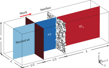
The computational domain and initial conditions are sketched in figure 1. The incident shock, initially at $z=-L/2$, propagates along the $z$-direction at the shock Mach number $M_{S}=1.5$. The initial pre-shock state is given by the stagnation pressure $p_0=23\,000$ Pa and temperature $T_0=298$ K. The corresponding post-shock density

(2.13)\begin{equation} \rho_{S}=\frac{\left(\bar{\gamma}+1\right)M_{S}^2}{2+\left(\bar{\gamma}-1\right)M_{S}^2}\rho_1, \end{equation}

pressure

(2.14)\begin{equation} p_{S}=\frac{2\bar{\gamma}M_{S}^2-\bar{\gamma}+1}{\bar{\gamma}+1}p_0 \end{equation}

and velocity $\boldsymbol {U}_{S}=U_{S}\boldsymbol {k}$ with

(2.15)\begin{equation} U_{S}=\frac{2\left(M_{S}^2-1\right)}{\left(\gamma_1+1\right)M_{S}}\sqrt{\frac{\gamma_1 p_0}{\rho_1}} \end{equation}

are calculated by the Rankine–Hugoniot conditions (see Courant & Friedrichs Reference Courant and Friedrichs1999).

Figure 1.

Schematic diagram of the computational domain and initial conditions.

2.3. Simulation methods

We apply the high-order turbulence solver (HOTS) developed by Liu & Xiao (Reference Liu and Xiao2016) to calculate (2.1)–(2.4). The HOTS employs a sixth-order compact finite difference scheme for spatial differentiation with an eighth-order compact filter to ensure the numerical stability (Shankar, Kawai & Lele Reference Shankar, Kawai and Lele2011). The localized artificial diffusivities (LADs) (Kawai & Lele Reference Kawai and Lele2008; Olson & Lele Reference Olson and Lele2013), which are calculated from the filtered local flow field, are added to corresponding physical ones $\bar {\mu }$, $\beta$, $\bar {\mathcal {K}}$ and $D_i$ in (2.5), (2.6) and (2.8). The LADs increase near the shock and interface to resolve physical discontinuities, while they are negligible in smooth regions to ensure the high numerical accuracy. A third-order total-variation-diminishing Runge–Kutta (TVD-RK) scheme (Gottlieb & Shu Reference Gottlieb and Shu1998) for temporal integration. We remark that the HOTS can act as a DNS if the grid resolution satisfies the DNS criterion (e.g. Groom & Thornber Reference Groom and Thornber2021) and the gird convergence test, while it is downgraded to an implicit large-eddy simulation if the flow field is under-resolved because the LAD can serve as a subgrid-scale model (Cook Reference Cook2007). The HOTS has been validated to be stable and reasonably accurate for DNS of RMI at $M_{S}\le 1.6$ (Liu & Xiao Reference Liu and Xiao2016; Peng et al. Reference Peng, Yang, Wu and Xiao2021), and $M_{S}$ can be further increased (e.g. $M_{S}\ge 2$) by using the shock-resolved technique to solve the NS equations (see Kramer et al. Reference Kramer, Pullin, Meiron and Pantano2010).

In the present simulation, the number of grid points for $\mathcal {D}$ is $N^2\times N$ with $N=256$ and ${\rm \Delta} x=L/N\approx 3.91\times 10^{-4}$ m, and the long sponge layer at $z<-L$ or $z>L$ is discretized by $N$ hyperbolic stretching grid points in the $z$-direction (see Liu & Xiao Reference Liu and Xiao2016). The total simulation time is $t=20$ ms, and the time stepping is ${\rm \Delta} t=2.5\times 10^{-4}$ ms satisfying the Courant–Friedrichs–Lewy (CFL) condition. To keep the interface approximately stationary near the middle of $\mathcal {D}$, the post-shock velocity $U_0^+ = 157.3\ {\rm m}\ {\rm s}^{-1}$ of the interface driven by the shock (Yang, Zhang & Sharp Reference Yang, Zhang and Sharp1994) is subtracted from the initial velocity in the $z$-direction, where $U_0^+$ is estimated by solving a one-dimensional Riemann problem.

The turbulent mixing in the RMI can be characterized by the growth of the mixing width (e.g. Thornber et al. Reference Thornber, Drikakis, Youngs and Williams2010)

(2.16)\begin{equation} W(t)=\int \langle Y_1 \rangle _{xy}(z,t) \langle Y_2 \rangle _{xy}(z,t)\,\mathrm{d} z, \end{equation}

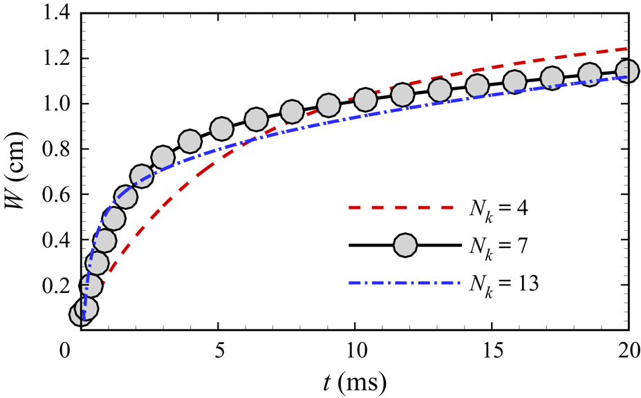
where $\langle \cdot \rangle _{xy}$ denotes the average over the $x$–$y$ plane in $\mathcal {D}$. The temporal evolutions of $W(t)$ for different initial perturbations with $N_k=4, 7$ and 13 in figure 2 show that the transition to the self-similar growth stage characterized by (1.1) becomes faster with larger $N_k$.

Figure 2.

Comparison of temporal evolutions of the mixing width with different initial perturbations $N_k=4, 7$ and 13.

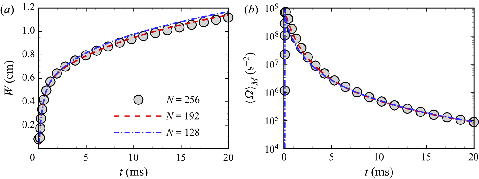
To examine the grid convergence with $N=128$, 192 or 256, we confirm that the profiles of the mixing width $W(t)$ and averaged enstrophy $\langle \varOmega \rangle _{M}(t)$ for the case with the broadband perturbation $N_k=13$ converge at $N=256$ in figure 3. Here, $\varOmega =|\boldsymbol{\omega }|^2/2$ denotes the enstrophy with the vorticity $\boldsymbol{\omega }=\boldsymbol{\nabla }\times \boldsymbol{u}=\omega _x\boldsymbol {i}+\omega _y\boldsymbol {j}+\omega _z\boldsymbol {k}$ and

(2.17)\begin{equation} \langle {\boldsymbol{\mathsf{f}}} \rangle _{M}(t)=\frac{1}{V_{M}}\int_\mathcal{M}\mathrm{d} z\int\!\!\!\!\!\int{\boldsymbol{\mathsf{f}}}(\boldsymbol{x},t)\,\mathrm{d}\kern0.06em x\mathrm{d} y \end{equation}

denotes the volume-averaged quantity ${\boldsymbol{\mathsf{f}}}(\boldsymbol{x},t)$ over the mixing zone with the volume $V_{M}=\int _\mathcal {M}\mathrm {d} z\int \!\!\!\int \mathrm {d}\kern0.06em x\,\mathrm {d} y$, where the mixing zone is defined as (see Tritschler et al. Reference Tritschler, Olson, Lele, Hickel, Hu and Adams2014a)

(2.18)\begin{equation} \mathcal{M}=\left\{z\,|\,4 \langle Y_1 \rangle _{xy}(z) \langle Y_2 \rangle _{xy}(z)\ge 0.9\right\}. \end{equation}

In addition, the criterion based on the scaled Kolmogorov scale $k_{max}\eta \ge 1$, widely used to validate DNS of the turbulent mixing induced by RMI (e.g. Tritschler et al. Reference Tritschler, Olson, Lele, Hickel, Hu and Adams2014a; Liu & Xiao Reference Liu and Xiao2016), is satisfied with $N=256$, where $k_{max }=3/{\rm \Delta} x$ is the maximum wavenumber (see Yeung & Pope Reference Yeung and Pope1989) and $\eta =( \langle \bar {\nu } \rangle _{M}^3/ \langle \epsilon \rangle _{M})^{1/4}$ is the Kolmogorov length scale with the mixture kinematic viscosity $\bar {\nu }=\bar {\mu }/\rho$ and the local dissipation rate $\epsilon =(\boldsymbol {\tau }:{\boldsymbol{\mathsf{S}}})/\rho$. Moreover, the resolution $N=256$ also satisfies the criterion proposed by Groom & Thornber (Reference Groom and Thornber2019, Reference Groom and Thornber2021) based on the initial Reynolds number.

Figure 3.

Grid convergence tests based on the temporal evolution of the (a) mixing width and (b) volume-averaged enstrophy in the mixing zone with $N_k=13$.

The energy cascade is characterized by the two-dimensional spectrum $E_k(k,t)$ of the kinetic energy $E_{K}=|\boldsymbol{u}|^2/2$ in terms of the radial wavenumber $k=\sqrt {k_x^2+k_y^2}$, and this spectrum is averaged over all the $x$–$y$ planes within the mixing zone in (2.18) along the $z$-direction (see Tritschler et al. Reference Tritschler, Olson, Lele, Hickel, Hu and Adams2014a). 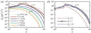The temporal evolution of $E_k(\kappa )$ in the case with $N_k=7$ is shown in figure 4, where $\kappa =k(L/2{\rm \pi} )$ is the scaled wavenumber. We find that the slope of $E_k$ in a narrow range of intermediate wavenumbers increases after the shock accelerates the interface at $t_{S}=t_{I}+\delta t_{I}=0.11$ ms and reaches the maximum $-3/2$ around $t^*=2$ ms, where $t_{I}$ and $\delta t_{I}$ are determined in (A1) and (A2), respectively. Then, the slope decreases and reaches the $-5/3$ law around $t=10$ ms when the flow becomes the fully developed HIT. The statistical isotropy in $x$–$y$ planes is supported by $\langle u' \rangle _{M}\approx \langle v' \rangle _{M}$ (not shown), where $u'$ and $v'$ are the root-mean-square fluctuating velocities in the $x$- and $y$-directions, respectively. At late times, the HIT decays with diminishing $E_k$.

Figure 4.

Comparisons of kinetic energy spectra. (a) At different times with the intermediate-band perturbation $N_k=7$. (b) With different initial perturbations at $t=t^*=2$ ms.

By comparing $E_k$ at $t^*=2$ ms from different initial perturbations of $N_k=4, 7$ and 13 in figure 4(b), we find that the cases with $N_k=7$ and 13 have the narrow region at intermediate wavenumbers with a slope closed to $-3/2$, and this region is broadened with $N_k$ and more evident with increasing $M_{S}$ (e.g. Thornber et al. Reference Thornber, Drikakis, Youngs and Williams2010; Oggian et al. Reference Oggian, Drikakis, Youngs and Williams2015). Therefore, the case with the intermediate-band perturbation $N_k=7$ can reveal the typical features of the multi-mode RMI, which is used for studying physical mechanisms and determining model parameters in the following discussion. We remark that the region of $E_k$ with a clear scaling law at intermediate wavenumbers may be narrow in turbulent mixing induced by RMI (e.g. Tritschler et al. Reference Tritschler, Hickel, Hu and Adams2013, Reference Tritschler, Zubel, Hickel and Adams2014b; Oggian et al. Reference Oggian, Drikakis, Youngs and Williams2015; Groom & Thornber Reference Groom and Thornber2021), because the Reynolds number is low when the incident shock is not strong. In this study, the averaged Taylor Reynolds number in the mixing zone is $\langle Re_\lambda \rangle _{M}\approx 230$ with $N_k=7$ after the shock accelerating the interface. It exceeds critical values $100\sim 140$ in the criterion proposed by Dimotakis (Reference Dimotakis2000), suggesting the independence of intermediate scales from the large and viscous scales.

3.1. Vorticity-based simplified models

In the RMI with a single-mode light/heavy interface accelerated by a weak incident shock, Peng et al. (Reference Peng, Yang, Wu and Xiao2021) demonstrated that the instability and asymmetric growth of the interface are mainly caused by the density difference and the PBV, whereas the pressure perturbation from distorted waves can be neglected. To distinguish the role of each factor in the present multi-mode RMI, we apply two vorticity-based simplified models, the double-density model (DDM) and the single-density model (SDM), which were developed in Peng et al. (Reference Peng, Yang, Wu and Xiao2021).

In the DDM, the initial condition involves post-shock quantities across the interface, including $T_1^+=426.88$, $T_2^+=339.36$ K and $p_0^+=75\,063$ Pa estimated by the one-dimensional Riemann problem along the $z$-direction (e.g. Yang et al. Reference Yang, Zhang and Sharp1994). Then, $\rho _i^+=p_0^+M_i/(\mathcal {R}T_i^+)$ is calculated by (2.9). In the SDM, uniform $\bar {\rho }^+=(\rho _1^++\rho _2^+)/2$ and $\bar {T}^+=(T_1^++T_2^+)/2$ are used for the initial condition.

The initial velocity of the DDM and SDM corresponds to that of the RMI at $t=t_{S}$ after the PBV is deposited. The PBV is generated by the interaction of the shock and interface. Taking the curl of (2.2) yields the vorticity equation

(3.1)\begin{equation} \frac{\textrm{D} \boldsymbol{\omega}}{\textrm{D} t}=\boldsymbol{B}+\boldsymbol{T}, \end{equation}

where $\mathrm {D}/\mathrm {D} t= {\partial }/ {\partial } t+\boldsymbol{u}\boldsymbol {\cdot }\boldsymbol{\nabla }$ denotes the material derivative,

(3.2)\begin{equation} \boldsymbol{B}=\frac{1}{\rho^2}\left(\boldsymbol{\nabla}\rho\times\boldsymbol{\nabla} p\right), \end{equation}

denotes the baroclinic term and

(3.3)\begin{equation} \boldsymbol{T}=\boldsymbol{\omega}\cdot\boldsymbol{\nabla}\boldsymbol{u}-\boldsymbol{\omega}(\boldsymbol{\nabla}\boldsymbol{\cdot}\boldsymbol{u})+\bar{\nu}\nabla^2\boldsymbol{\omega}, \end{equation}

denotes the ‘non-baroclinic’ term containing stretching, dilatation and viscous terms.

From (3.1), we derive the PBV (detailed in Appendix A)

(3.4)\begin{equation} \boldsymbol{\omega}_{PB}=\frac{8{\rm \pi}\beta_\omega A^+{\rm \Delta} p^+}{\bar{\rho}^+L\left(M_{S} \sqrt{\dfrac{\gamma_1 p_0}{\rho_1}}-U_0^+\right)} \delta(\varphi_{I}^+)\left[K_x(x,y)\boldsymbol{i}+K_y(x,y)\boldsymbol{j}\right], \end{equation}

with

(3.5)$$\begin{gather} K_x(x,y)=\sum_{n=1}^{N_k}\sum_{m=1}^{N_k+2}\frac{k_n L}{2{\rm \pi}}a_{n,m}\cos(k_n x+\phi_n)\sin(k_m y+\chi_m), \end{gather}$$

(3.6)$$\begin{gather}K_y(x,y)=\sum_{n=1}^{N_k}\sum_{m=1}^{N_k+2}\frac{k_m L}{2{\rm \pi}}a_{n,m}\sin(k_n x+\phi_n)\cos(k_m y+\chi_m) \end{gather}$$

and the Dirac function $\delta (\cdot )$. Since effects of the pressure perturbation, such as three-wave nodes (see Samtaney & Zabusky Reference Samtaney and Zabusky1993, Reference Samtaney and Zabusky1994; Samtaney, Ray & Zabusky Reference Samtaney, Ray and Zabusky1998), and the finite thickness of the interface can change the PBV magnitude in the multi-mode RMI, a non-dimensional correction factor $\beta _\omega$ is introduced in (3.4) to make the PBV magnitude equal to the vorticity magnitude in the RMI generated just after the shock accelerates the interface. Hence, $\beta _\omega$ is determined by $\langle |\boldsymbol{\omega }_{PB}| \rangle = \langle |\boldsymbol{\omega }| \rangle$ at $t=t_{S}$, where $\langle \cdot \rangle$ denotes the volume average in $\mathcal {D}$, and $\langle |\boldsymbol{\omega }| \rangle$ at $t=t_{S}$ is directly determined from the simulation results of the RMI. For $N_k=4, 7$ and 13, we obtain $\beta _\omega =4.15\times 10^{-4}, 3.09\times 10^{-4}$ and $3.01\times 10^{-4}$, respectively.

The initial velocity

(3.7)\begin{equation} \boldsymbol{u}_{PB}(\boldsymbol{x})=\mathscr{T}_{BS}\{\boldsymbol{\omega}_{PB}(\boldsymbol{x})\} \end{equation}

of the DDM and SDM is induced by the PBV, where

(3.8)\begin{equation} \mathscr{T}_{BS}\{\boldsymbol{\omega}_{PB}(\boldsymbol{x})\}=\frac{1}{4{\rm \pi}}\int_\mathcal{D} \frac{\boldsymbol{\omega}_{PB}(\boldsymbol{x}')\times(\boldsymbol{x}'-\boldsymbol{x})}{|\boldsymbol{x}'-\boldsymbol{x}|^3}\,\mathrm{d}\kern0.06em x'\,\mathrm{d} y'\,\mathrm{d} z' \end{equation}

denotes the operation of the Biot–Savart (BS) law with $\boldsymbol{x}'=x'\boldsymbol {i}+y'\boldsymbol {j}+z'\boldsymbol {k}$. Given the periodic $\boldsymbol{\omega }_{PB}$ in $\mathcal {D}$, (3.8) can be written as (see Xiong & Yang Reference Xiong and Yang2019)

(3.9)\begin{equation} \mathscr{T}_{BS}\{\boldsymbol{\omega}_{PB}(\boldsymbol{x})\}=\mathscr{F}^{{-}1} \left\{\frac{\textrm{i}\boldsymbol{k}_{F}\times\mathscr{F}\{\boldsymbol{\omega}_{PB}(\boldsymbol{x})\}}{\left|\boldsymbol{k}_{F}\right|^2}\right\}, \end{equation}

with the Fourier transform operator $\mathscr {F}\{\cdot \}$, the inverse Fourier transform operator $\mathscr {F}^{-1}\{\cdot \}$ and the wavenumber $\boldsymbol {k}_{F}$ in the Fourier space. The schematic comparison of the initial conditions of the RMI, DDM and SDM is shown in figure 5. Without the shock in $\mathcal {D}$, the effects of pressure perturbations from distorted waves are only modelled by $\beta _\omega$ in (3.4), which alters the PBV magnitude in the DDM and SDM.

Figure 5.

Schematic comparison of the initial conditions of (a) RMI, (b) DDM and (c) SDM, where IF denotes the interface and IS the incident shock.

3.2. Comparison of RMI, DDM and SDM

The simulations of DDM and SDM are essentially the same as the DNS of RMI except for the different initial conditions and the removal of sponge layers. Since the incident shock is weak, it will be demonstrated in § 4.2 that the compressibility effect can be negligible. Hence, there is almost no effect of pressure perturbations by compression waves in the DDM and SDM with the solenoidal initial velocity (3.7). In order to characterize the asymmetric growth of the mixing zone, we further decompose (2.16) into $W(t)=W_{s}(t)+W_{b}(t)$, where integral widths of spikes

(3.10)\begin{equation} W_{s}(t)=\int_{ \langle Y_1 \rangle > \langle Y_2 \rangle } \langle Y_1 \rangle _{xy}(z,t) \langle Y_2 \rangle _{xy}(z,t)\,\mathrm{d} z \end{equation}

and bubbles

(3.11)\begin{equation} W_{b}(t)=\int_{ \langle Y_1 \rangle < \langle Y_2 \rangle } \langle Y_1 \rangle _{xy}(z,t) \langle Y_2 \rangle _{xy}(z,t)\,\mathrm{d} z \end{equation}

are separated by the interface defined as the isosurface of $Y_1=Y_2$ (Lombardini, Pullin & Meiron Reference Lombardini, Pullin and Meiron2014).

The temporal evolution of $W_{s}(t)$ and $W_{b}(t)$ in the DDM and SDM is compared with that in the corresponding RMI with $N_k=7$ in figure 6, where $t_{S}$ is subtracted from the time for RMI. We observe that $W_{s}(t)$ and $W_{b}(t)$ grow asymmetrically in the DDM, which are nearly identical to those in the RMI except for slight over-predictions, whereas they are symmetric in the SDM.

Figure 6.

Temporal evolution of the widths of (a) spikes and (b) bubbles with $N_k=7$ from the RMI and the corresponding DDM and SDM.

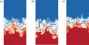
The distributions of the mass fraction of air on the slice $x=0$ in the RMI, DDM and SDM are compared at a late time $t=20$ ms in figure 7, together with interfaces (isosurfaces of $Y_1=Y_2$). We observe asymmetric spike and bubble regions across the interface in the RMI and DDM and the statistically symmetric distribution of $Y_1$ in the SDM, consistent with the mean profiles in figure 6.

Figure 7.

Comparison of the mass fraction of air (colour coded by $0\le Y_1\le 1$ from blue through white to red) on the slice $x=0$ with $N_k=7$ from the (a) RMI, (b) DDM and (c) SDM. The grey line denotes the interface defined by the isosurface of $Y_1=Y_2=0.5$.

The consistent results in RMI and DDM demonstrate that the present multi-mode RMI with a weak incident shock is mainly driven by the synergistic effect of the density difference across the perturbed interface and the PBV (see §§ 4.2 and 4.3 in Peng et al. Reference Peng, Yang, Wu and Xiao2021), whereas the pressure perturbation from distorted waves only plays a minor role in reducing the growth rate (e.g. Velikovich et al. Reference Velikovich, Dahlburg, Schmitt, Gardner, Phillips, Cochran, Chong, Dimonte and Metzler2000) and their effect on the PBV distribution is neglected. Therefore, the DDM can serve as a simplified model for the present multi-mode RMI. It is noted that the DDM calculation does not need the long sponge layers, and its computational cost is approximately half of that for the simulation of RMI in the present study. Furthermore, we compare the compensated energy spectra in the RMI, DDM and SDM in figure 8. It is clear that, at $t^*=2$ ms, both spectra in the RMI and DDM have slopes close to $-3/2$ in the narrow ranges of intermediate wavenumbers, whereas the corresponding slope in the SDM is close to $-5/3$ as in the HIT. On the other hand, at a late time $t=10$ ms, the slopes in the narrow regions in all the cases are close to $-5/3$. In addition, similar results are found in the cases with the narrowband and broadband perturbations $N_k=4$ and 13 (not shown).

Figure 8.

Comparison of kinetic energy spectra from the RMI, DDM and SDM with $N_k=7$ at (a) $t=t^*=2$ and (b) $t=10$ ms.

We have demonstrated that the significant difference between the RMI and HIT at the critical time $t^*=2$ ms is not directly generated by the shock, because there is no shock in the DDM. Therefore, the SBV generated in the DDM (see Peng et al. Reference Peng, Yang, Wu and Xiao2021) is essential to produce the $-3/2$ law in the RMI instead of the $-5/3$ law in the HIT.

4.1. SBV

In the present RMI without reshock, the SBV arises after the shock accelerates the interface (see Peng et al. Reference Peng, Yang, Wu and Xiao2021). Distinguished from the PBV, the generation of the SBV is due to the misalignment between the density gradient across the interface and the pressure gradient produced by the PBV-induced velocity.

Using the DDM, we calculate the SBV to demonstrate its important role in the growth of the mixing zone. From the Lagrangian view, $\boldsymbol{\omega }$ can be obtained by integrating the right-hand side of (3.1) and decomposing into

(4.1)\begin{equation} \boldsymbol{\omega}=\boldsymbol{\omega}_0(\boldsymbol{x})+\boldsymbol{\omega}_{SB}(\boldsymbol{x},t)+\boldsymbol{\omega}_{T}(\boldsymbol{x},t), \end{equation}

with the initial vorticity $\boldsymbol{\omega }_0(\boldsymbol{x})=\boldsymbol{\omega }_{PB}(\boldsymbol{x})$, the SBV

(4.2)\begin{equation} \boldsymbol{\omega}_{SB}(\boldsymbol{x},t)=\int_0^t\boldsymbol{B}(\boldsymbol{x},t')\,\mathrm{d} t' \end{equation}

defined by the temporal integral of the baroclinic term in the vorticity equation (3.1) and the vorticity component

(4.3)\begin{equation} \boldsymbol{\omega}_{T}(\boldsymbol{x},t)=\int_0^t\boldsymbol{T}(\boldsymbol{x},t')\,\mathrm{d} t' \end{equation}

excluding $\boldsymbol{\omega }_0$ and $\boldsymbol{\omega }_{SB}$.

In this way, the enstrophy $\varOmega =|\boldsymbol{\omega }|^2/2$ is decomposed into

(4.4)\begin{equation} \varOmega(\boldsymbol{x},t)=\varOmega_0(\boldsymbol{x})+\varOmega_{SB}(\boldsymbol{x},t)+\varOmega_{T}(\boldsymbol{x},t)+\varOmega_{C}(\boldsymbol{x},t), \end{equation}

with the initial enstrophy $\varOmega _0=|\boldsymbol{\omega }_0|^2/2$, the SBV enstrophy $\varOmega _{SB}=|\boldsymbol{\omega }_{SB}|^2/2$, the ‘non-SBV’ enstrophy $\varOmega _{T}=|\boldsymbol{\omega }_{T}|^2/2$ and the cross-component $\varOmega_{C}=\boldsymbol{\omega }_{SB}\cdot \boldsymbol{\omega }_{T}+\boldsymbol{\omega }_0\cdot (\boldsymbol{\omega }_{SB}+\boldsymbol{\omega }_{T})$.

Figure 9 plots the temporal evolution of averaged magnitudes of $\boldsymbol {B}$ and $\boldsymbol {T}$ in the vorticity equation (3.1), and the enstrophy components $\varOmega _{SB}$ and $\varOmega _{T}$ in the DDM. Although instantaneous $\langle |\boldsymbol {B}| \rangle _{M}$ is always smaller than $\langle |\boldsymbol {T}| \rangle _{M}$, $\varOmega _{SB}$, as a measure of the temporal integral of $\boldsymbol {B}$, is more dominant than $\varOmega _{T}$ in the enstrophy variation. This implies a persistent SBV effect on the evolution of the RMI.

Figure 9.

Temporal evolution of volume-averaged (a) magnitudes of the baroclinic and ‘non-baroclinic’ terms in (3.1) and (b) components $\varOmega _{SB}$ and $\varOmega_{C}$ of the enstrophy variation in (4.4) in the mixing zone.

4.2. Effects of SBV on the kinetic energy spectrum

In figure 9(b), the SBV enstrophy peaks around $t^*=2$ ms, coinciding with the appearance of the $-3/2$ scaling law of $E_k$ in figure 4(a). Next, we elucidate the effects of the SBV on the energy spectrum.

First, we apply the Helmholtz decomposition (e.g. Moyal Reference Moyal1952) to the velocity field as

(4.5)\begin{equation} \boldsymbol{u}(\boldsymbol{x},t)=\boldsymbol{u}_{s}(\boldsymbol{x},t)+\boldsymbol{u}_{d}(\boldsymbol{x},t), \end{equation}

where the solenoidal component $\boldsymbol{u}_{s}=\mathscr {T}_{BS}\{\boldsymbol{\omega }\}$ is induced by $\boldsymbol{\omega }$ with $\boldsymbol{\nabla }\boldsymbol {\cdot }\boldsymbol{u}_{s} = 0$ and the dilatational component $\boldsymbol{u}_{d}$ satisfies $\boldsymbol{\nabla }\times \boldsymbol{u}_{d} = 0$. Based on (4.5), we decompose the kinetic energy $E_{K}=E_{K,s}+E_{K,d}$ into the solenoidal component $E_{K,s}=|\boldsymbol{u}_{s}|^2/2$ and the dilatational one $E_{K,d}=|\boldsymbol{u}_{d}|^2/2$. The temporal evolution of $\langle E_{K,s} \rangle _{M}$ and $\langle E_{K,d} \rangle _{M}$ in figure 10(a) shows that $\langle E_{K,d} \rangle _{M}$ is smaller than $\langle E_{K,s} \rangle _{M}$ by two orders of magnitude, so we have the approximation $\boldsymbol{u} = \mathscr {T}_{BS}\{\boldsymbol{\omega }\}$, i.e. the compressibility effect on the velocity can be neglected.

Figure 10.

Temporal evolution of volume-averaged (a) solenoidal and dilatational components of the kinetic energy, and (b) components of the kinetic energy variation in (4.7).

In this way, the velocity is approximated by applying the BS law (3.8) to (4.1) as

(4.6)\begin{equation} \boldsymbol{u}(\boldsymbol{x},t) = \boldsymbol{u}_0(\boldsymbol{x})+\boldsymbol{u}_{SB}(\boldsymbol{x},t)+\boldsymbol{u}_{T}(\boldsymbol{x},t) \end{equation}

with $\boldsymbol{u}_0=\mathscr {T}_{BS}\{\boldsymbol{\omega }_{PB}\}$, $\boldsymbol{u}_{SB}=\mathscr {T}_{BS}\{\boldsymbol{\omega }_{SB}\}$ and $\boldsymbol{u}_{T}=\mathscr {T}_{BS}\{\boldsymbol{\omega }_{T}\}$. Similar to (4.4), the kinetic energy of (4.6) is decomposed into

(4.7)\begin{equation} E_{K}(\boldsymbol{x},t)=E_{K,0}(\boldsymbol{x})+E_{K,SB}(\boldsymbol{x},t)+E_{K,T}(\boldsymbol{x},t)+E_{K,C}(\boldsymbol{x},t), \end{equation}

where $E_{K,0}=|\boldsymbol{u}_0|^2/2$ denotes the initial kinetic energy, $E_{K,SB}=|\boldsymbol{u}_{SB}|^2/2$ the kinetic energy induced by the SBV, $E_{K,T}=|\boldsymbol{u}_{T}|^2/2$ the kinetic energy induced by the non-SBV vorticity component and $E_{K,C}=\boldsymbol{u}_0\cdot (\boldsymbol{u}_{SB}+\boldsymbol{u}_{T})+\boldsymbol{u}_{SB}\cdot \boldsymbol{u}_{T}$ the cross component.

Figure 10(b) plots the temporal evolution of $\langle E_{K,SB} \rangle _{M}$, $\langle E_{K,T} \rangle _{M}$ and $\langle E_{K,C} \rangle _{M}$. We find that the decay of $\langle E_{K,s} \rangle _{M}$ in figure 10(a) is mainly caused by negative $E_{K,C}$. On the contrary, $E_{K,SB}$ and $E_{K,T}$ make positive contributions to the kinetic energy, where $E_{K,SB}$ dominates and peaks at $t=t^*$, coinciding with the time when $\langle \varOmega _{SB} \rangle _{M}$ peaks in figure 9(b). Thus, the growth of $E_{K,SB}$ at $t\le t^*$ mitigates the energy decay around $t=t^*$ in figure 10(a).

We analyse the SBV effects on the kinetic energy spectrum. For given $\boldsymbol{\omega }(\boldsymbol{x},t)$ at a particular time $t$, the vorticity

(4.8)\begin{equation} \boldsymbol{\omega}(\boldsymbol{x},t+\delta t)=\boldsymbol{\omega}(\boldsymbol{x},t)+\delta\boldsymbol{\omega}_{SB}(\boldsymbol{x},t)+\delta\boldsymbol{\omega}_{T}(\boldsymbol{x},t) \end{equation}

at $t+\delta t$ is calculated by the temporal integral of (3.1), where the vorticity variation during $\delta t$ is, similar to (4.1), decomposed into the SBV component

(4.9)\begin{equation} \delta\boldsymbol{\omega}_{SB}(\boldsymbol{x},t)=\int_t^{t+\delta t}\boldsymbol{B}(\boldsymbol{x},t')\,\mathrm{d} t', \end{equation}

and the non-SBV component

(4.10)\begin{equation} \delta\boldsymbol{\omega}_{T}(\boldsymbol{x},t)=\int_t^{t+\delta t}\boldsymbol{T}(\boldsymbol{x},t')\,\mathrm{d} t'. \end{equation}

Applying the BS law (3.8) to (4.8) yields

(4.11)\begin{equation} \boldsymbol{u}(\boldsymbol{x},t+\delta t)=\boldsymbol{u}(\boldsymbol{x},t)+\delta\boldsymbol{u}_{SB}(\boldsymbol{x},t)+\delta\boldsymbol{u}_{T}(\boldsymbol{x},t), \end{equation}

with $\delta \boldsymbol{u}_{SB}=\mathscr {T}_{BS}\{\delta \boldsymbol{\omega }_{SB}\}$ and $\delta \boldsymbol{u}_{T}(\boldsymbol{x},t)=\mathscr {T}_{BS}\{\delta \boldsymbol{\omega }_{T}\}$. Similar to (4.4), the kinetic energy variation based on (4.11) is decomposed into

(4.12)\begin{equation} E_{K}(\boldsymbol{x},t+\delta t)=E_{K}(\boldsymbol{x},t)+\delta E_{K,SB}(\boldsymbol{x},t)+ \delta E_{K,T}(\boldsymbol{x},t)+\delta E_{K,C}(\boldsymbol{x},t), \end{equation}

where $\delta E_{K,SB}=|\delta \boldsymbol{u}_{SB}|^2/2$ denotes the kinetic energy variation caused by the SBV, $\delta E_{K,T}=|\delta \boldsymbol{u}_{T}|^2/2$ the kinetic energy variation caused by non-SBV terms and $\delta E_{K,C}=\delta \boldsymbol{u}_{SB}\cdot \delta \boldsymbol{u}_{T}+\boldsymbol{u}\cdot \left (\delta \boldsymbol{u}_{SB}+\delta \boldsymbol{u}_{T}\right )$ the cross-component.

Hence, (4.12) is a generalized expression of (4.7) during an arbitrary period from $t$ to $t+\delta t$. According to the analysis of (4.7) and figure 10, the accumulation of $\delta E_{K,SB}$ with time influences the evolution of the kinetic energy during $t\le t^*$. To show the SBV effects on the energy cascade, we transform (4.12) into the Fourier space and then obtain the decomposition of the kinetic energy spectrum

(4.13)\begin{equation} E_k(k,t+\delta t)=E_k(k,t)+\delta E_{k,SB}(k,t)+\delta E_{k,T}(k,t)+\delta E_{k,C}(k,t). \end{equation}

We consider the contribution of $\delta \boldsymbol{u}_{SB}(\boldsymbol{x},t)$ to $E_k(k,t+\delta t)$ in each time step in the numerical simulation with $\delta t={\rm \Delta} t$. In figure 11(a), the spectra $\delta E_{k,SB}(k,t)$ of the kinetic energy variations induced by the SBV show a clear $-1$ scaling law at small and intermediate wavenumbers before $t = t^*$ when the SBV-component of the enstrophy variation reaches the maximum. After $t = t^*$, $\delta E_{k,SB}$ decays sharply at large wavenumbers.

Figure 11.

Effects of the SBV on the compensated kinetic energy spectra. (a) Spectra of the kinetic energy variations from the SBV at different times. (b) Comparison of the spectra of the kinetic energy variations from the SBV in the RMI and the spectra of the total kinetic energy in the DDM and SDM at $t^*=2$ ms.

By comparing $\delta E_{k,SB}$ and $E_k$ in the DDM and SDM at $t^*=2$ ms in figure 11(b), we observe that $E_{k,DDM}$ is close to the $-3/2$ law at intermediate wavenumbers owing to the incremental compensation of $\delta E_{k,{SB}}$ with the $-1$ law through (4.13) at each time step. By contrast, $E_{k,{SDM}}$ without the SBV effect is closer to the $-5/3$ law as that in the HIT. The diminishing SBV effects after $t = t^*$, as implied in figures 10(b) and 11(a), cause the kinetic energy spectrum to evolve towards the $-5/3$ law in figure 4(a). We remark that $\delta E_{k,{SB}}$ does not show a fast decaying tail at high wavenumbers in figure 11. A possible reason is that the gradients in (3.2) are not fully resolved at small scales. However, this numerical artefact in the postprocessing of simulation data has negligible effects on the observation of the $-1$ law at intermediate wavenumbers.

4.3. Vortex reconnection in the mixing zone

To explain the $-1$ scaling law of $\delta E_{k,{SB}}$ before the critical time $t = t^*$, we investigate the vortex dynamics in the mixing zone using the VSF method (see Yang & Pullin Reference Yang and Pullin2010), which has been applied to investigate Lagrangian-like vortex dynamics in transitional wall flows (Zhao, Yang & Chen Reference Zhao, Yang and Chen2016), combustion (Zhou et al. Reference Zhou, You, Xiong, Yang, Thévenin and Chen2019), magnetohydrodynamics (Hao, Xiong & Yang Reference Hao, Xiong and Yang2019) and single-mode RMI (Peng et al. Reference Peng, Yang, Wu and Xiao2021). The VSF $\phi _v(\boldsymbol{x},t)$ is a smooth scalar satisfying the constraint $\boldsymbol{\omega }\boldsymbol {\cdot }\boldsymbol{\nabla }\phi _v=0$, where $\boldsymbol{\omega }$ is tangent on the isosurface of $\phi _v$ except for vorticity nulls, i.e. each VSF isosurface is a vortex surface consisting of vortex lines.

Based on the PBV in (3.4), the initial VSF for the DDM is set to (see Peng et al. Reference Peng, Yang, Wu and Xiao2021)

(4.14)\begin{equation} \phi_{v0}(\boldsymbol{x})=\frac{z}{a_0^+}-\eta(x,y)\exp\left\{-[\varphi_{I}^+(\boldsymbol{x})]^{2m}\right\}, \end{equation}

with a weighting index $m=10$. The evolution of the VSF in this multi-mode RMI is calculated by the two-time method (Yang & Pullin Reference Yang and Pullin2011). The numerical implementation is described in Appendix B. The accuracy of the numerical VSF solutions at $0< t\le t^*$ is satisfactory, according to the small averaged VSF deviation $\langle |\lambda _\omega | \rangle _{M}<10\,\%$ (see Yang & Pullin Reference Yang and Pullin2010) in the mixing zone with $\lambda _{\omega }\equiv (\boldsymbol{\omega }\boldsymbol {\cdot }\boldsymbol{\nabla }\phi _v)/(|\boldsymbol{\omega }||\boldsymbol{\nabla }\phi _v|)$.

The evolution of the VSF isosurface $\phi _v=0$ colour coded by $0\le |\boldsymbol{\omega }|/|\boldsymbol{\omega }|_{max }\le 0.8$ is shown in figure 12 during $0\le t\le t^*$. This vortex surface coincides with the interface at $t=0$ in the DDM in figure 12(a), and the distribution of $|\boldsymbol{\omega }|= |\boldsymbol{\omega }_{PB}|$ on the surface has large variations. Then, with the persistent effect of the SBV, the vorticity on the vortex surface grows asymmetrically, forming spikes and bubbles at $t=0.4$ ms in figure 12(b). In this period, the spikes and bubbles evolve independently as in the single-mode RMI (see Peng et al. Reference Peng, Yang, Wu and Xiao2021). Subsequently, the vortex reconnections occur at scattered locations. For example, two inclined spikes $S_1$ and $S_2$, highlighted in figure 12(b), merge at $t=1.2$ ms, as highlighted in the dashed circle in figure 12(c). The large values of $|\boldsymbol{\omega }|$ on the vortex surface (in red) around the reconnection region implies the large local dissipation with $\epsilon \approx \bar {\nu }|\boldsymbol{\omega }|^2 = 2\bar {\nu }\varOmega$ in this study. At $t = t^*=2$ ms, the vortex-reconnection events among spikes spread all over the vortex surface in the mixing zone in figure 12(d), and the peaks of volume-averaged enstrophy components around $t^* = 2$ ms in figure 9(b) suggest the highest volume-averaged dissipation rate. Finally, the vortical structures become more convoluted and trigger turbulent mixing.

Figure 12.

Temporal evolution of the vortex surface $\phi _v=0$ at (a) $t=0$, (b) $t=0.4$ ms with two typical spikes $S_1$ and $S_2$, (c) $t=1.2$ ms when the incipient vortex reconnection of $S_1$ and $S_2$ occurs (highlighted in the dotted circle) and (d) $t=t^*=2$ ms when the vortex reconnection widely occurs in the mixing zone. The vortex surfaces are colour coded by $0\le |\boldsymbol{\omega }|/|\boldsymbol{\omega }|_{max }\le 0.8$ from blue through white to red.

The vortex reconnection is also illustrated by the contour of $\omega _x$ on the slice at $x=0.015$ m in figure 13. The PBV in figure 13(a) grows asymmetrically due to the SBV (see Peng et al. Reference Peng, Yang, Wu and Xiao2021) and generates spikes and bubbles at $t=0.4$ ms in figure 13(b). The vortex reconnections between different spikes or bubbles occur sparsely at $t=1.2$ ms, as highlighted in red dashed squares in figure 13(c), and the reconnections spread in the entire mixing zone at $t = t^*=2$ ms in figure 13(d).

Figure 13.

Temporal evolution of $\omega _x$ (colour coded by $-0.8\le \omega _x/\omega _{x,\textit{max} }\le 0.8$ from blue through white to red) at (a) $t=0$ with the generation of the PBV, (b) $t=0.4$ ms with almost independent spikes and bubbles, (c) $t=1.2$ ms when the incipient vortex reconnections occur (highlighted in red dotted squares) and (d) $t=t^*=2$ ms when the vortex reconnections widely occur in the mixing zone.

Hence, $t=t^*$ is also a critical time when vortex reconnections widely occur in the mixing zone, coinciding with the maximal SBV effect on the kinetic energy spectrum. During $t< t^*$, most spikes and bubbles evolve independently as in the single-mode RMI, so the direction of $\boldsymbol {B}$ in (3.1) does not vary significantly and the SBV integrated by $\boldsymbol {B}$ persistently grows with time. The emergence of vortex reconnections at $t=t^*$, with interactions between different spikes and bubbles in the turbulent mixing, rapidly changes the direction of $\boldsymbol {B}$ and mitigates the SBV effect.

4.4. Modelling SBV effects on the kinetic energy spectrum

Since spikes and bubbles evolve almost independently during $t< t^*$, we model them using a square array of $N_k^2$ vortex rings. This modelling approach, developed in Peng et al. (Reference Peng, Yang, Wu and Xiao2021) for the single-mode RMI, is sketched in figure 14. The motion of each vortex ring is characterized by the moving dual polar coordinates in figure 15. This coordinate system moves with the vortex ring. The central axis of the vortex ring is described by polar coordinates $(R,\theta )$ with the origin at the ring centre. The cross-section of the ring is described by polar coordinates $(r,\varphi )$ with the origin at the central axis of the ring. For the time-varying radius $R(t)$ of the vortex ring, these coordinates are spanned by $(r,\varphi ,\theta )$ with unit basis $\boldsymbol {e}_r$, $\boldsymbol {e}_\varphi$ and $\boldsymbol {e}_\theta$.

Figure 14.

The schematic diagram for the modelling of spikes and bubbles in the multi-mode RMI. (a) Close-up view of the almost independently evolving spikes and bubbles (marked in the dash-dotted square in figure 12b). (b) The model of vortex rings developed in Peng et al. (Reference Peng, Yang, Wu and Xiao2021). (c) Close-up view of the contour of $\omega _x$ on the slice of the vortex ring at $x=0$ (marked in the dotted square in figure 13b) with the centre $C_j$, radius $r_{C,j}$ and the characteristic length scale $\ell _{SB,j}$.

Figure 15.

Schematic diagram of the moving dual polar coordinates, consisting of (a) polar coordinates for the vortex ring $(R,\theta )$ and (b) polar coordinates on a cross-section of the ring $(r,\varphi )$. The red arrow denotes the direction of movement of the vortex ring.

When spikes and bubbles evolve independently before reconnection, each spike or bubble, e.g. the spike highlighted in figure 14(a), can be modelled as in the single-mode RMI in figure 14(b). According to Peng et al. (Reference Peng, Yang, Wu and Xiao2021), we assume the vorticity $\boldsymbol{\omega }=\omega _\theta (r,t)\boldsymbol {e}_\theta$ and the induced velocity $\boldsymbol{u}=u_\varphi (r,t)\boldsymbol {e}_\varphi$ of the vortex ring are uniform in the $\theta$-direction. For each spike or bubble labelled by the subscript ‘$j$’ with $j=1,2,\ldots ,N_k^2$, we model

(4.15a,b)\begin{gather} \omega_{\theta,j}(r_j,t)=\frac{\varGamma_j(t)}{4{\rm \pi}\bar{\nu}t}\exp \left(-\frac{r_j^2}{4\bar{\nu}t}\right)\quad \text{and}\quad u_{\varphi,j}(r_j,t)=\frac{\varGamma_j(t)}{2{\rm \pi} r_j}\left[1-\exp\left(-\frac{r_j^2}{4\bar{\nu}t}\right)\right] \end{gather}

by Gaussian distributions in terms of the distance $r_j$ from the central axis of the $j$th vortex ring to the location where $\omega _j$ peaks, where $\varGamma _j$ denotes the circulation of each spike or bubble.

We consider the vorticity variation

(4.16)\begin{align} \delta\omega_{\theta,j}(r_j,t)&=\omega_{\theta,j}(r_j,t+\delta t)-\omega_{\theta,j}(r_j,t) \nonumber\\ &=\frac{\varGamma_j(t+\delta t)}{4{\rm \pi}\bar{\nu}(t+\delta t)}\exp \left[-\frac{r_j^2}{4\bar{\nu}(t+\delta t)}\right]-\frac{\varGamma_j(t)}{4{\rm \pi}\bar{\nu}t} \exp\left(-\frac{r_j^2}{4\bar{\nu}t}\right) \end{align}

from $t$ to $t+\delta t$, where the circulation variation $\delta \varGamma _j(t)=\varGamma _j(t+\delta t)-\varGamma _j(t)$ is produced by the SBV variation $\delta \omega _{{SB},j}$ with $\delta \boldsymbol{\omega }_{{SB},j}=\delta \omega _{{SB},j}\boldsymbol {e}_\theta$. Peng et al. (Reference Peng, Yang, Wu and Xiao2021) demonstrated that the SBV dominates the vorticity variation. Compared with $\delta \varGamma _j(t)$, the viscous diffusion of $\omega _{\theta ,j}$ can be ignored during $\delta t$, so (4.16) is approximated by

(4.17)\begin{equation} \delta\omega_{\theta,j}(r_j,t)=\frac{\delta\varGamma_j(t)}{4{\rm \pi}\bar{\nu}t} \exp\left(-\frac{r_j^2}{4\bar{\nu}t}\right), \end{equation}

and the velocity variation

(4.18)\begin{equation} \delta u_{\varphi,j}(r_j,t)=\frac{\delta\varGamma_j(t)}{2{\rm \pi} r_j}\left[1-\exp\left(-\frac{r_j^2}{4\bar{\nu}t}\right)\right] \end{equation}

induced by $\delta \omega _{\theta ,j}$ is obtained.

Next, we model the characteristic length scale $\ell _{{SB},j}$ of the SBV variation in the mixing zone. The characteristic length scale of $\delta \omega _{\theta ,j}$ can be modelled by the radial distance

(4.19)\begin{equation} r_{C,j}=2\sqrt{\bar{\nu}t} \end{equation}

from the ring centre to the location where $\delta u_{\varphi ,j}$ peaks. As $\delta \omega _{\theta ,j}$ is dominated by $\delta \varGamma _j$, which is produced by $\delta \omega _{{SB},j}$, $r_{C,j}$ is also a characteristic length scale of $\delta \omega _{{SB},j}$, as marked by the blue arrow in figure 14(c). Then considering the definition of the two-dimensional energy spectrum, $\ell _{{SB},j}$ is calculated by the averaged projection of $r_{C,j}$ onto the $x$–$y$ plane as

(4.20)\begin{equation} \ell_{SB,j}\propto\frac{1}{2{\rm \pi}}\int_0^{2{\rm \pi}}\left|r_{C,j}\cos\varphi\right|\,\mathrm{d}\varphi= \frac{\rm \pi}{2}r_{C,j}, \end{equation}

as shown by the yellow arrow in figure 14(c).

Substituting (4.19) to (4.20) yields

(4.21)\begin{equation} \ell_{SB,j}\propto(\bar{\nu}\tau_{SB})^{1/2}, \end{equation}

where the characteristic time scale $\tau _{SB}$ of $\delta \omega _{SB,j}$ is used. The characteristic wavenumber corresponding to the $j$th vortex ring for a spike or bubble can be expressed as

(4.22)\begin{equation} k\propto \ell_{SB,j}^{{-}1}\propto(\bar{\nu}\tau_{SB})^{{-}1/2}, \end{equation}

and then we have

(4.23)\begin{equation} \tau_{SB}\propto k^{{-}2}\bar{\nu}^{{-}1}. \end{equation}

Substituting (4.23) into the generalized kinetic energy spectrum (see Zhou Reference Zhou2001) in (1.5) with $\tau _{T}(k) = \tau _{SB}$ yields the spectrum of the kinetic energy variation from the SBV as

(4.24)\begin{equation} \delta E_{k,SB}\propto k^{{-}1}(\bar{\nu}\varepsilon)^{1/2}. \end{equation}

Thus, we obtain the $-1$ scaling law of $\delta E_{k,SB}$, consistent with the simulation results in figure 11, by modelling the scale of the SBV variation in the mixing zone based on the motion of vortex rings.

5.1. Model development

In the mixing zone of the multi-mode RMI, we have demonstrated that the essential vortex dynamics involves almost independently evolving vortex rings during $t\le t^*$, and then vortex reconnections around $t=t^*$ trigger turbulent mixing. These findings inspire us to improve the existing model (1.2) of the mixing width. First, the mixing width during $t\le t^*$ is modelled by the motion of vortex rings for spikes and bubbles as in the single-mode RMI (see Peng et al. Reference Peng, Yang, Wu and Xiao2021), instead of the linear growth model. Second, this vortex-ring model is matched with the self-similar law of the mixing width at $t=t^*$, instead of the ad hoc choice of the matching time. Thus, (1.2) is improved by

(5.1)\begin{equation} W(t)=\left\{ \matrix{& W_0+\int_0^t\dot{W}_{R}(t')\,\mathrm{d} t',\hfill & t\le t^* \cr & W^*\left[1+\frac{\dot{W}^*}{\theta_W W^*}\left(t-t^*\right)\right]^{\theta_W} & t>t^*,} \right. \end{equation}

where $\dot {W}_{R}$ is the interfacial growth rate based on vortex rings in the single-mode RMI, and $W^*=W(t^*)$ and $\dot {W}^*=\dot {W}(t^*)$ are the mixing width and its growth rate at $t=t^*$, respectively.

During $t\le t^*$, Peng et al. (Reference Peng, Yang, Wu and Xiao2021) estimated the growth rates of spikes/bubbles as

(5.2)\begin{equation} \dot{W}_{s/b}(t)=\frac{\varGamma_{s/b}(t)}{4{\rm \pi} R_0} \left[1-\exp\left(-\frac{\alpha_3 R_0^2}{\bar{\nu}t}\right)\right] \left[\log\frac{4R_0}{\sqrt{\bar{\nu}\left(t+t_\varepsilon\right)}}-0.558\right] \end{equation}

with

(5.3)\begin{equation} \varGamma_{s/b}(t)=\varGamma_0\left[\alpha_1\pm\alpha_2\left(\frac{\dot{W}_0t}{R_0}\right)^{({3\pm 1}/{4})A^+}\right], \end{equation}

where the positive/negative sign respectively applies to spikes/bubbles. In this model, the SBV effect is introduced by the increasing/decreasing of the spike/bubble circulation $\varGamma _{s/b}(t)$ in (5.3), which leads to the asymmetric growths of spike and bubble widths. Here, the initial circulation

(5.4)\begin{equation} \varGamma_0=\frac{(4+2{\rm \pi})\beta_\omega A^+W_0{\rm \Delta} p^+}{M_{S}\bar{\rho}^+} \sqrt{\frac{\rho_1}{\gamma_1 p_0}} \end{equation}

is evaluated by that in the single-mode RMI (Peng et al. Reference Peng, Yang, Wu and Xiao2021) with the additional correction of $\beta _\omega$. The average radius of the vortex rings is estimated by

(5.5)\begin{equation} R_0=\frac{L}{2{\rm \pi} N_k} \end{equation}

based on the initial perturbation (2.11). The average kinematic viscosity in the mixing zone is calculated by

(5.6)\begin{equation} \bar{\nu}=\frac{\bar{\mu}}{\bar{\rho}^+}=\frac{\mu_1\sqrt{M_2}+\mu_2\sqrt{M_1}}{\bar{\rho}^+ \left(\sqrt{M_1}+\sqrt{M_2}\right)}, \end{equation}

where $\bar {\mu }$ is calculated from Reid et al. (Reference Reid, Pransuitz and Poling1987), and $\mu _1$ and $\mu _2$ are respectively determined at $T_1^+$ and $T_2^+$. Moreover, a small drift time $t_\varepsilon$ is used to remove the temporal singularity at $t=0$. We remark that the growth of RMI in (5.2) mainly depends on the effect of $A^+$ in (5.3) (see Peng et al. Reference Peng, Yang, Wu and Xiao2021), and the growth is slightly mitigated by the viscous effect via changing the vorticity distribution (e.g. Niederhaus & Jacobs Reference Niederhaus and Jacobs2003; Movahed & Johnsen Reference Movahed and Johnsen2013). The model parameters $\alpha _1=2131.1$, $\alpha _2=639.3$ and $\alpha _3=5.201\times 10^{-4}$ in (5.2) are determined by the simulation results with the intermediate-band perturbation $N_k=7$.

Then, we obtain the model of $\dot {W}_{R}=\dot {W}_{s}+\dot {W}_{b}$ as

(5.7)\begin{equation} \dot{W}_{R}=\frac{\varGamma(t)}{4{\rm \pi} R_0}\left[1-\exp\left({-}5.2\times 10^{{-}4} \frac{R_0^2}{\bar{\nu}t}\right)\right]\left[\log\frac{4R_0}{\sqrt{\bar{\nu}\left(t+t_\varepsilon\right)}}-0.558\right], \end{equation}

with

(5.8)\begin{equation} \varGamma(t)=\varGamma_0\left\{2131+639.3\left[\left(\frac{\dot{W}_0t}{R_0}\right)^{A^+}- \left(\frac{\dot{W}_0t}{R_0}\right)^{A^+{/}2}\right]\right\}, \end{equation}

and

(5.9)\begin{equation} t_\varepsilon=\frac{16R_0^2}{\bar{\nu}}\exp\left({-}7.5\times 10^{{-}3}{\rm \pi}\frac{R_0\dot{W}_0}{\varGamma_0}-1.116\right) \end{equation}

determined from $\dot {W}_{s}(0)=\dot {W}_{b}(0)=\dot {W}_0/2$.

The vortex-reconnection time $t^*$ in (5.1) for matching the vortex-based model of $W(t)$ at early times and the power law of $W(t)$ at late times is estimated by the time when two approaching vortex surfaces merge together (see Zhao et al. Reference Zhao, Yang and Chen2016). As shown in figure 13, the merging of vortex surfaces between adjacent spikes or bubbles is caused by the radius growth of vortex rings. Since the averaged initial distance between adjacent spikes or bubbles is equal to $R_0$ in (5.5), we model $t^*$ by the time when the average radius of vortex rings, which is proportional to $\sqrt {\bar {\nu }t}$ from (4.19), grows to $R_0$ in the mixing zone. Thus, we have

(5.10)\begin{equation} R_0 = \alpha_{R}\sqrt{\bar{\nu}t^*}, \end{equation}

where the model parameter $\alpha _{R} = 19.60$ is determined by $t^*=2\ {\rm ms}$ and $R_0=2.3\times 10^{-3}\ {\rm m}$ from the numerical results of the case with $N_k=7$. Then, the reconnection time is modelled by

(5.11)\begin{equation} t^*=2.6\times 10^{{-}3}\frac{R_0^2}{\bar{\nu}}. \end{equation}

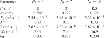
The model parameters in (5.1) are summarized in table 1 with their physical meanings and determination methods. We remark that the prediction of the power-law exponent $\theta _W$ of the mixing width in the self-similar growth region remains an open problem (e.g. Jacobs et al. Reference Jacobs, Krivets, Tsiklashvili and Likhachev2013; Weber, Cook & Bonazza Reference Weber, Cook and Bonazza2013; Oggian et al. Reference Oggian, Drikakis, Youngs and Williams2015), so it has to be fitted from the simulation data at late times.

Table 1.

Summary of parameters in the model (5.1) of the mixing width with (5.7).

5.2. Model assessment

The proposed model (5.1) is assessed by the three simulation cases with various initial perturbation modes. All the model parameters listed in table 2 are calculated from the initial simulation data except for $\theta _W$. Implied by (5.5) and (5.11), $t^*$ decreases with increasing $N_k$.

Table 2.

Model parameters for the three simulation cases with different modes of the initial perturbation.

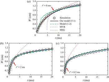
In figure 16, our model results (solid lines) agree with the simulation (symbols) for various $N_k$, where $t_{S}$ is subtracted from the time for numerical results. The two sub-models of (5.1), the vortex-ring model for $t\le t^*$ and the self-similar growth model for $t>t^*$, match at $t=t^*$. For comparison, we also plot the results of the existing model (1.2) in figure 16, where the matching time $t_{c}$ is determined by (1.4) as $t_{c}=1.7$, 0.60 and 0.14 ms by tuning the free model parameter $\beta _W=1165$, 410.7 and 93.93 to best fit the simulation results.

Figure 16.

Comparison of the present model (5.1) and the existing model (1.2) for estimating the mixing width, along with results of the three simulation cases with (a) $N_k=4$, (b) $N_k=7$ and (c) $N_k=13$. The present model matches two sub-models, the model based on the motion of vortex rings (MVR) and the model of the self-similar growth (MSG), at $t=t^*$ (marked by arrows).

We observe that our model captures the nonlinear growth of $W(t)$ at early times via modelling the motion of vortex rings for spikes and bubbles. This result is more accurate than the linear growth in the existing model, and this advantage is notable for narrowband perturbations with small $N_k$. In addition, the matching time $t^*$ in the present model is determined by (5.11) when the vortex reconnection widely occurs, which avoids tuning the free parameter in (1.4) for different cases. Therefore, the present model (5.1), incorporating the vortex-based growth model (5.7) and the vortex-reconnection time (5.11), can estimate the mixing width in the multi-mode RMI with various modes of the initial perturbation.