1 Introduction
1.1 Literature review
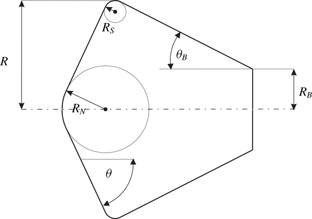
Atmospheric entry capsules shaped as spherically blunted, large apex-angle cones are widely used in space missions. Therefore, the hypersonic flow over this class of shapes has been studied extensively. Depending on flow conditions and cone angle, the shock shape and the shape of the sonic line are dominated either by the spherical nose or the conical part. The most obvious changes accompanied by the transition between these two situations is an increase in shock stand-off distance and a movement of the sonic point on the body surface from the spherical part to the shoulder. In this section we list and describe the results of the rich record of work on this problem. A typical shape is shown in figure 1.
Schematic sketch of spherically blunted cone capsule. The spherical nose is tangent to the large apex-angle cone.

South (Reference South1968) conducted computations of supersonic and hypersonic flow of an ideal gas past different blunt bodies with sonic corners, i.e. subsonic forebody flow at zero angle of attack. The numerical scheme was based on an integral method and surface pressure distributions, the shape and location of the detached bow shock wave, and the forebody pressure drag coefficient were determined and compared to experiment. Particular emphasis was put on spherically blunted cones of large apex angle and the change of characteristic flow features caused by variation of either the cone angle or the specific heat ratio were discussed. If conditions regarding cone angle or specific heat ratio were selected such that for a pointed cone an attached oblique shock wave and fully supersonic flow would develop, inflection points were detected on the shock wave of the blunted cone beyond the sphere–cone junction. Simultaneously, the surface pressure distributions revealed a relative minimum just ahead of the sphere–cone junction followed by a large recompression beyond the junction. For these conditions, the solution in the nose region was dominated by the sphere with constant dimensionless shock stand-off distance, however, for increasing cone angle or specific heat ratio, beyond the sonic condition for a pointed cone, the shock stand-off distance continuously increased. Further, the inflection points on the shock wave disappeared and the relative minimum and recompression of the surface pressure were reduced and ultimately vanished. For a
 $60^{\circ }$
blunted cone, the drag, pressure distribution, shock stand-off distance and stagnation-point velocity gradient were further investigated as functions of the nose bluntness ratio. Regarding the drag, it was pointed out that the Newtonian theory significantly overestimates the effect of bluntness.
The correlation between the appearance of shock wave inflection points and surface pressure recompression for supersonic and hypersonic flows past blunted cones up to cone angles of
 $30^{\circ }$
and with supersonic flow in the recompression region – contrary to the study by South (Reference South1968) where the flow on the forebody was always subsonic – was analysed numerically by Traugott (Reference Traugott1962) also using an integral method. As pointed out by South (Reference South1968), compared to his subsonic shock layer flow cases, in Traugott’s results the shock wave inflection point is located further downstream because, in the supersonic flow, the information of the recompression is transported to the shock along the outgoing compression characteristic which reaches the shock further downstream. In the case of subsonic flow, the recompression appeared at the shock almost immediately.
Krasil’nikov, Nikulin & Kholodov (Reference Krasil’nikov, Nikulin and Kholodov1975) conducted numerical calculations of hypersonic flow of calorically perfect gases over spherically blunted cones with cone angles above
 $40^{\circ }$
and zero angle of attack. The unsteady gas dynamic equations were solved using a time stepping scheme without imposing the restrictions on the position of the sonic point along the forebody surface in the studies of South and Traugott. The forebody shapes considered consisted of a spherical nose and a conical section followed by a cylindrical part. Since the vertical extent of the spherical section was kept constant in relation to the base radius, a changing cone angle implies increased nose bluntness. The shock wave and sonic line shapes as well as the resulting surface pressure distributions were discussed for varying cone angle and specific heat ratio. At the smallest angle the sonic point on the body surface was identical to the one on an isolated sphere. With increasing cone angle, an elongated subsonic regime developed, extending along the conical part close to the wall. At their largest cone angle of
 $70^{\circ }$
, the shock layer was completely subsonic with the sonic point located at the shoulder. The dimensionless wall pressure distributions revealed similar characteristics as those reported by South (Reference South1968). For the low cone angle cases, a relative minimum with subsequent recompression developed near the junction between the spherical and conical parts. For the
 $70^{\circ }$
case, the pressure dropped continuously along the surface. This effect was explained by the influence of centrifugal forces on the spherical part. Further, for a constant cone angle of
 $60^{\circ }$
, the variation of shock stand-off distance, sonic line shape and wall pressure distributions were discussed. Qualitatively similar results as for the changing cone angle cases were obtained. Using the Newtonian and Newton–Busemann theories, the qualitative and quantitative characteristics of the wall pressure distributions obtained with computational fluid dynamics could not be reproduced.
The forebody shape of the Mars Pathfinder entry configuration was a
 $70^{\circ }$
half-angle cone with base diameter 2.65 m, nose radius 0.6638 m and shoulder radius 0.06625 m (Braun et al.
Reference Braun, Powell, Cruz, Gnoffo and Weilmuenster1995). The spacecraft conducted a direct spin stabilized entry from its interplanetary flight path, i.e. no active control was used. The post-flight analysis of its hypersonic aerodynamic database in the continuum flow regime was presented by Gnoffo et al. (Reference Gnoffo, Braun, Weilmuenster, Mitcheltree, Engelund and Powell1999). It was pointed out that the pre-flight prediction of two static aerodynamic instability intervals along the entry trajectory were confirmed by acceleration measurements conducted during the Pathfinder entry flight (see also, e.g. Spencer et al.
Reference Spencer, Thurman, Peng, Blanchard and Braun1998). As discussed in Braun et al. (Reference Braun, Powell, Cruz, Gnoffo and Weilmuenster1995) and Gnoffo et al. (Reference Gnoffo, Weilmuenster, Braun and Cruz1996), these instabilities are associated with a movement of the sonic line on the leeward forebody side and, at small angles of attack, from the shoulder to the nose region and back. It was further outlined that the sonic line location is a function of the trajectory point considered and the corresponding shock layer gas chemistry which changes along the hypersonic flight trajectory path from frozen to equilibrium. The evaluation of their numerical results revealed that the movement of the sonic point from the spherical part to the shoulder starts with the development of a subsonic bubble in the shock layer just downstream of an inflection point in the bow shock wave. Subsequently the bubble expands to merge with the subsonic region at the boundary layer edge, and the bow shock inflection point disappears. The sonic line movement goes along with a changing surface pressure distribution. In particular, the difference of the surface pressure in the vicinity of the windward and leeside shoulders can, under certain conditions, result in a destabilizing pitching moment.
In Braun et al. (Reference Braun, Powell, Cruz, Gnoffo and Weilmuenster1995) it was noted that a similar static instability region as found for the Mars Pathfinder entry configuration was also predicted in the Viking program based on ballistic range tests. Viking 1 and 2 conducted their Mars atmospheric entry flights in 1976, and they were the first in a series of subsequent United States Mars entry vehicles, including Mars Pathfinder, Mars Exploration Rovers, Phoenix and the Mars Science Laboratory, to use a
 $70^{\circ }$
sphere-cone forebody and identical nose bluntness (nose radius to base radius ratio:
 $R_{N}/R_{B}=0.5$
). Compared to their successors, the Viking vehicles have a smaller shoulder bluntness (shoulder radius to base radius ratio:
 $R_{s}/R_{B}=0.0145$
compared to
 $R_{s}/R_{B}=0.05$
). In his computational analysis of the Viking lander capsule hypersonic aerodynamics, Edquist (Reference Edquist2006) reported that within the velocity range for which the Mars Pathfinder static instabilities were predicted, the Viking aerodynamics revealed that the trim angle is sensitive to changes in free-stream density. It was concluded that these changes of the atmospheric density affect the equilibrium state of the post-shock gas and may, therefore, explain the observed sensitivity. At lower hypersonic flight Mach numbers this sensitivity was not observed.
While the entry velocity of the Mars Exploration Rovers was smaller than that of Mars Pathfinder, two similar static instability regions due to sonic line movement on the leeward side of the forebody were identified in the hypersonic flight regime. As outlined by Schoeneberger, Cheatwood & Desai (Reference Schoeneberger, Cheatwood and Desai2005), these instabilities are caused by changes in the forebody pressure distribution because the gas chemistry behaviour changed from frozen flow to equilibrium (Mach 27) and from equilibrium to perfect-gas flow (Mach 16). In contrast to the spin stabilized entry flights of Mars Pathfinder and the Mars Exploration Rovers flying at a nominal
 $0^{\circ }$
trim angle, the Mars Science Laboratory conducted an actively guided entry (Dyakonov, Schoeneberger & Norman Reference Dyakonov, Schoeneberger and Norman2012). Lift was generated by off-setting the centre of mass, resulting in a hypersonic trim at approximately
 $16^{\circ }$
.
Further space missions using blunted-cone capsules include the Russian Mars 3 spacecraft which conducted its mission in 1971. The configuration consisted of a
 $60^{\circ }$
half-cone angle, 3.2 m diameter lander forebody (Perminov Reference Perminov1999). The NASA sample return capsule Genesis collected a sample of solar wind particles and returned them to Earth in 2004. The Stardust aerodynamic database served as the basis for the aerodynamics of the Genesis
 $60^{\circ }$
sphere-cone capsule with a nose radius of
 $R_{N}=0.442~\text{m}$
, a diameter of
 $D=2R_{B}=1.52~\text{m}$
and a shoulder radius of
 $R_{s}=0.034~\text{m}$
(Desai & Cheatwood Reference Desai and Cheatwood2001). The Huygens capsule conducted its entry into the atmosphere of Saturn’s moon Titan as part of the joint NASA/ESA Cassini/Huygens program in 2005. The NASA Stardust sample return capsule conducted its Earth re-entry in 2006. The blunted
 $60^{\circ }$
half-angle sphere-cone configuration had a nose radius of
 $R_{N}=0.2202~\text{m}$
, a diameter of
 $D=0.811~\text{m}$
and a shoulder radius of
 $R_{s}=0.02~\text{m}$
(Mitcheltree et al.
Reference Mitcheltree, Wilmoth, Cheatwood, Brauckmann and Greene1997). The forebody consisted of a
 $60^{\circ }$
sphere-cone geometry with a nose radius of
 $R_{N}=1.25~\text{m}$
, a diameter of
 $D=2.7~\text{m}$
and a shoulder Radius of
 $R_{s}=0.05~\text{m}$
(Powell et al.
Reference Powell, Justus, Bose, Chen, Cruz, Duvall, Fisher, Hollis, Lockwood and Keller2005). On the Japanese Hayabusa (MUSES-C) sample return capsule forebody a spherically blunted cone with nose bluntness of
 $R_{N}/R_{B}=1.0$
was used (Ishii et al.
Reference Ishii, Yamada, Hiraki and Inatanii2008). The base diameter was 404 mm and the cone half-angle was
 $45^{\circ }$
. The Schiaparelli entry, descent and landing demonstrator module of the ExoMars mission which was conducted by ESA in cooperation with the Russian Space Agency Roskosmos in 2016, consisted of a 2.4 m diameter,
 $70^{\circ }$
sphere-cone front shield and a
 $47^{\circ }$
conical back shield. The aeroshape was close to that of the Viking landers, with a slight difference in the shoulder radius (
 $R_{s}/D=0.025$
instead of 0.0073 for Viking) and in the rear cone (simple cone of
 $47^{\circ }$
for ExoMars and bi-cone of
 $40^{\circ }/62.18^{\circ }$
for Viking). As pointed out by Tran & Beck (Reference Tran and Beck2011), ExoMars aerodynamics thus took advantage of a high historical heritage.
In addition to the characterization of the aerodynamic behaviour of blunted-cone capsule configurations, a series of studies focused on the experimental and numerical prediction of shock shapes, shock stand-off distances and wall heat flux distributions in reacting carbon dioxide flows. Laminar and turbulent wall heat flux distributions were measured on a
 $70^{\circ }$
blunt-cone wind tunnel model representing the scaled forebody of the Mars Science Laboratory (MSL) in the T5 shock tunnel of the California Institute of Technology (Wright et al.
Reference Wright, Olejniczak, Brown, Hornung and Edquist2005). The results confirmed the occurrence of the leeside turbulent heat flux augmentation which was predicted in computations at flight conditions. However, open questions remained regarding the modelling of the catalytic properties of the model surface for the laminar and turbulent cases.
Holden et al. (Reference Holden, Wadhams, MacLean and Mundy2007) observed measured shock shapes and stand-off distances that differed significantly from numerical simulations of flow over a MSL scaled model in high-enthalpy conditions (5 and
 $10~\text{MJ}~\text{kg}^{-1}$
) in the Large Energy National Shock Tunnel I (LENS I) reflected shock tunnel. It was further discussed that when testing the same model in the LENS X expansion tube facility at
 $5~\text{MJ}~\text{kg}^{-1}$
excellent agreement was obtained between simulations and experiments. A similar approach also considering a scaled MSL configuration in an expansion tunnel by Sharma et al. (Reference Sharma, Swantek, Flaherty and Austin2010) provided complementary results to the work of Holden et al. (Reference Holden, Wadhams, MacLean and Mundy2007) and supported the conclusion that the discrepancy between reflected shock tunnel and expansion tunnel data is driven by the means by which the test gas is accelerated to hypervelocity speeds. However, recent experiments conducted in the T5 reflected shock tunnel (Leibowitz & Austin Reference Leibowitz and Austin2019) bracketed the conditions of the LENS I experiments and found excellent agreement with expansion tube data and with computations, thus reconfirming the utility of reflected shock tunnels for high-enthalpy carbon dioxide flows that had been established over many years by an extensive body of previous work from high-enthalpy shock tunnel laboratories (e.g. T3, T5, HEG, HIEST). In fact, a highly improbable degree of free-stream non-equilibrium would be required to explain the large anomaly of the LENS I result.
1.2 Objectives
The reported static instabilities of Mars entry configurations are not crucial for the success of the mission. However, they do increase the dispersion of the landing site prediction. For high precision landing missions, it is, therefore, important to obtain an in-depth understanding of the sphere-cone transition behaviour. In order to explore this phenomenon more systematically, we embark on a theoretical, numerical and experimental effort in order to obtain a clear picture of the features of this interesting flow. An important part of the issue is the flow over a sharp cone in the detached shock regime. The shock stand-off distance and drag coefficient on cones with large half-angles that are relevant to atmospheric entry capsules are insensitive to boundary layer effects. Such features may therefore be profitably investigated by computations of the inviscid flow using the Euler equations. This then is the topic of Part 1. Although the numerical study in Part 1 is performed with a calorically perfect gas, the results have relevance to non-equilibrium situations in the manner derived e.g. by Stulov (Reference Stulov1969) and Wen & Hornung (Reference Wen and Hornung1995).
Part 2 will cover the experimental and numerical investigation of the flow over a series of blunted-cone capsules. Detailed results of experiments in the high-enthalpy shock tunnel Göttingen (HEG) of the German Aerospace Centre using air as test gas will be presented. The experiments are performed at conditions where thermochemical non-equilibrium effects are significant. Accordingly, results will be compared to numerical predictions using different physical–chemical models. These computations also take viscous effects into account.
2 Background
Because of its paramount importance throughout Part 1, we introduce the inverse density ratio across a normal shock
 $$\begin{eqnarray}\unicode[STIX]{x1D700}=\frac{\unicode[STIX]{x1D70C}_{\infty }}{\unicode[STIX]{x1D70C}_{s}},\end{eqnarray}$$
which, for a calorically perfect gas, is
 $$\begin{eqnarray}\unicode[STIX]{x1D700}=\frac{\unicode[STIX]{x1D6FE}-1+2/M_{\infty }^{2}}{\unicode[STIX]{x1D6FE}+1}.\end{eqnarray}$$
Here,
 $\unicode[STIX]{x1D70C}$
is the density, subscripts
 $s$
and
 $\infty$
refer to immediate post shock and free stream, respectively;
 $\unicode[STIX]{x1D6FE}$
is the (constant) ratio of specific heats and
 $M$
is the Mach number.
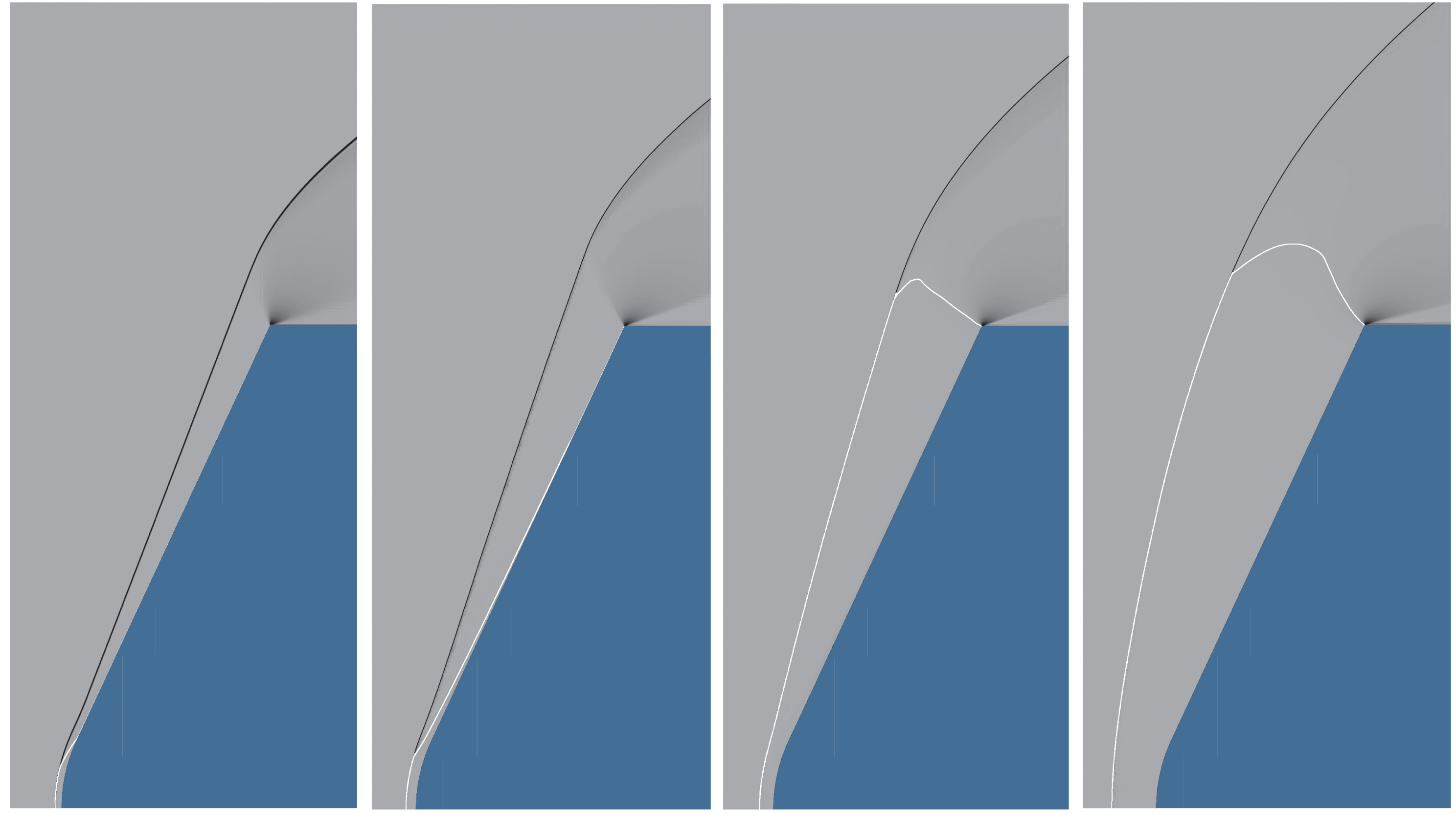
In order to illustrate the transition between sphere behaviour and cone behaviour, it is convenient to use results of Euler computations of the flow. Examples presented in figure 2 show this transition.
Pseudo-schlieren images from computations of inviscid perfect-gas flows over a
 $65^{\circ }$
spherically blunted cone with the ratio of the radius from the axis to the shoulder to the nose radius,
 $R/R_{N}=3$
at
 $M_{\infty }=10$
and (from left)
 $\unicode[STIX]{x1D6FE}=1.09$
, 1.15, 1.21 and 1.4, i.e. inverse normal-shock density ratio
 $\unicode[STIX]{x1D700}$
ranging from 0.0526 to 0.175. The sonic line is shown in white. Note how, in the first two frames on the left, the sonic line terminates either on the spherical part of the body or hugs the cone (sphere behaviour), while it reaches the shoulder at almost a right angle for the two larger values of
 $\unicode[STIX]{x1D6FE}$
(cone behaviour). During sphere behaviour, the shock wave has a straight portion that, if projected, intersects the axis at the same point as the projection of the cone surface.

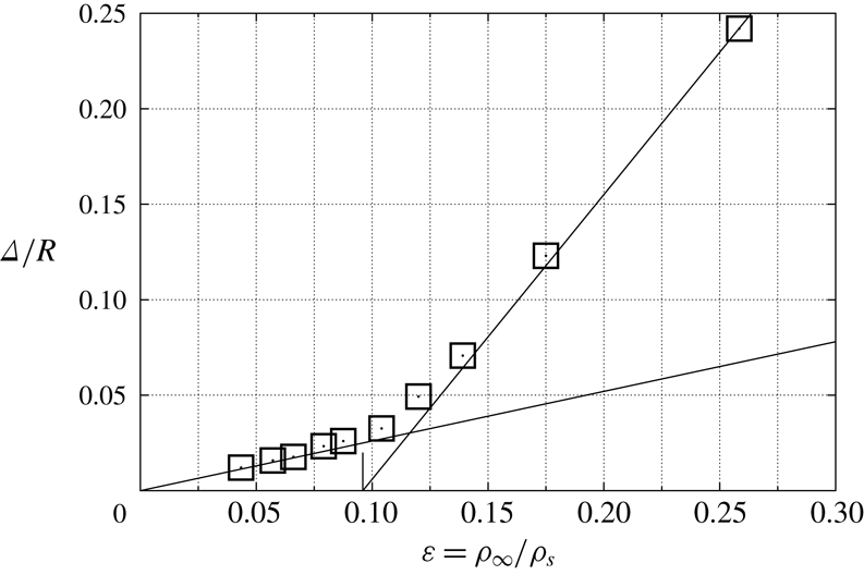
The difference between the two regimes is brought out nicely in a plot of the dimensionless shock wave stand-off distance,
 $\unicode[STIX]{x1D6E5}/R$
, where
 $\unicode[STIX]{x1D6E5}$
is the distance along the stagnation streamline of the shock from the stagnation point and
 $R$
is the radius from the axis to the shoulder, against
 $\unicode[STIX]{x1D700}$
. This plot is shown in figure 3 for
 $\unicode[STIX]{x1D703}=65^{\circ }$
. The straight line through the origin is the well-known relation
 $$\begin{eqnarray}\frac{\unicode[STIX]{x1D6E5}}{R_{N}}=0.78\unicode[STIX]{x1D700}\end{eqnarray}$$
for flow over a sphere (see e.g. Hornung Reference Hornung1972). The other straight line is drawn from the detachment condition (shown with a short vertical line on the abscissa) to fit the points in the cone behaviour regime.
Dimensionless stand-off distance, measured from computations like those of figure 2 and shown as open square symbols, plotted versus
 $\unicode[STIX]{x1D700}$
for a
 $65^{\circ }$
sphere-cone with
 $R/R_{N}=3$
. At small
 $\unicode[STIX]{x1D700}$
, the points fall on the straight line through the origin, equation (2.3) (sphere behaviour). At larger
 $\unicode[STIX]{x1D700}$
they depart drastically from this line. The short vertical line on the abscissa indicates the point
 $\unicode[STIX]{x1D700}=\unicode[STIX]{x1D700}_{d}$
, see (3.3), that corresponds to shock detachment from a sharp cone. A straight line has been drawn from this point to fit the cone behaviour at larger
 $\unicode[STIX]{x1D700}$
.

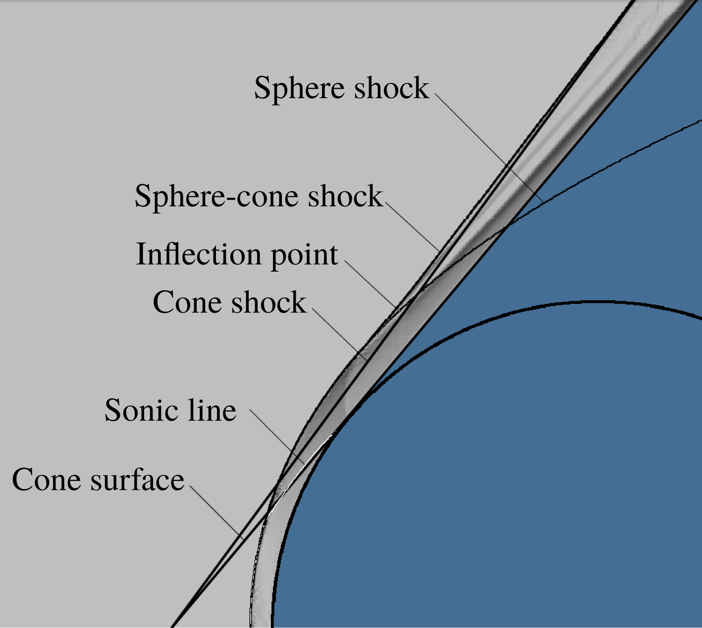
It is worth discussing the details of the appearance of a point of inflection in the shock wave, see also figure 2 left. In order to bring this out, figure 4 shows a superposition of results from computations of three flows. First, the results of a computation of a sphere-cone with half-angle
 $50^{\circ }$
and
 $R/R_{N}=3$
is inserted as a pseudo-schlieren image. Superimposed on this is the result from a computation of flow over a sharp
 $50^{\circ }$
cone tangent to the sphere. This shows only a particular contour of the density gradient that is chosen at a value such as to just select the shock wave. In the same fashion, the flow over a sphere is displayed. Common to the sphere flow and the sphere-cone flow in this situation is the sonic line, shown as a white line. First, note that the sphere-cone shock merges into the sharp-cone shock at large distances from the axis of symmetry (bottom edge of figure) and into the sphere shock at smaller distance. Because the sphere shock extends upstream of the cone shock at some point, this leads to a point of inflection in the sphere-cone shock. It is interesting that in the limit
 $\unicode[STIX]{x1D700}\rightarrow 0$
Freeman (Reference Freeman1960) showed that the shock layer on a sphere detaches from the body at the
 $60^{\circ }$
point and follows the shape
 $y\propto x^{1/3}$
. On a sphere-cone, such a shock layer would reimpinge on the conical part of the body (see e.g. Hornung Reference Hornung1969), so that a point of inflection would necessarily arise.
Overlay of computational results from flows over three different bodies: a sphere, a
 $50^{\circ }$
sphere-cone with the same nose radius as the sphere and a
 $50^{\circ }$
sharp cone, that is tangent to the sphere. The shock of the sphere-cone merges into the shock on the sphere near the axis of symmetry (bottom edge of figure) and into the sharp-cone shock at large radius.
 $M_{\infty }=10$
,
 $\unicode[STIX]{x1D6FE}=1.16$
,
 $\unicode[STIX]{x1D700}=0.0833$
.

Second, consider the point of intersection of the projection of the conical part of the surface of the sphere-cone (which is also the sharp-cone surface) with the projection of the far-field sphere-cone shock. Note that this intersection point lies on the axis. This is as it should be, because a sphere-cone with
 $R/R_{N}\rightarrow \infty$
behaves like a sharp cone and, in the range of sphere behaviour, so does the sphere-cone shock.
Two subtle points come out in the pseudo-schlieren image. One is that the part of the flow that has come through the strongly curved part of the shock wave shows up as a dark region near the sphere-cone surface. This is the so-called entropy layer, a region in which the entropy is higher than in the region where the flow has come through the almost straight part of the sphere-cone shock. This leads to increased density gradients that show up as darker regions in this representation.
The second is that there is a jump in surface curvature at the junction of the sphere with the cone, in this case just downstream of the sonic line. This causes a slight discontinuity of the density gradient in the flow that propagates along a characteristic toward the shock wave. It therefore shows up as a small discontinuity of grey shading along that characteristic. At the shock, this separates the part of the shock wave that is affected by the conical part of the sphere-cone from that which is not. No information about the conical part of the body reaches the region upstream of this characteristic. The converse is not true, because the displacement effect of the entropy layer changes the effective surface of the conical part of the sphere-cone. This displacement effect is small and asymptotically approaches zero as the surface of the conical part of the sphere-cone. This displacement effect is small and asymptotically approaches zero as the cone circumference increases with distance from the tip.
3 Theoretical considerations for flow over a cone
Consider steady inviscid flow of a perfect gas over a right circular cone of half-angle
 $\unicode[STIX]{x1D703}$
at zero angle of attack. If
 $\unicode[STIX]{x1D703}$
is sufficiently small, the shock wave on the cone is conical and attached to the cone tip, and the flow between the shock and the cone is supersonic. The flow details are described by the equations of Taylor & Maccoll (Reference Taylor and Maccoll1933). As
 $\unicode[STIX]{x1D703}$
is increased it reaches a point beyond which the flow is mixed, with a conical sonic surface between the shock and the body, see e.g. Solomon (Reference Solomon1953). Taylor–Maccoll solutions exist even up to the point where the whole flow between the shock and the body is subsonic, although they then only apply to a cone of infinite extent and are not relevant to the physical situation of a finite cone. Beyond an angle
 $\unicode[STIX]{x1D703}_{d}$
Taylor–Maccoll solutions do not exist. This is called the detachment angle because, for
 $\unicode[STIX]{x1D703}>\unicode[STIX]{x1D703}_{d}$
, the shock wave is detached and curved with a normal shock on the stagnation streamline. Let the cone extend to a sharp shoulder at radius
 $R$
from the axis. The flow is then subsonic up to a sonic line that extends between the shock wave and the shoulder, at which a centred expansion wave accelerates the flow, see figure 2 right.
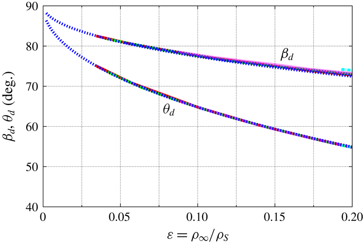
The conditions at the detachment point can be found by solving the Taylor–Maccoll equations. However, an excellent approximation is given by (Hayes & Probstein Reference Hayes and Probstein1959)
 $$\begin{eqnarray}\displaystyle & \displaystyle \unicode[STIX]{x1D6FD}_{d}=\arctan \sqrt{\frac{2}{\unicode[STIX]{x1D700}}}, & \displaystyle\end{eqnarray}$$
 $$\begin{eqnarray}\displaystyle & \displaystyle \unicode[STIX]{x1D703}_{d}=2\,\unicode[STIX]{x1D6FD}_{d}-\frac{\unicode[STIX]{x03C0}}{2}, & \displaystyle\end{eqnarray}$$
where
 $\unicode[STIX]{x1D6FD}$
is the (attached) shock angle that takes the value
 $\unicode[STIX]{x1D6FD}_{d}$
at the detachment point. Figure 5 illustrates the quality of these approximations, which is especially good in the case of
 $\unicode[STIX]{x1D703}_{d}$
. Thus,
 $\unicode[STIX]{x1D6FD}_{d}$
and
 $\unicode[STIX]{x1D703}_{d}$
which are functions of
 $M_{\infty }$
and
 $\unicode[STIX]{x1D6FE}$
, depend on these variables virtually only in the particular combination in
 $\unicode[STIX]{x1D700}$
, (2.2). With a given
 $\unicode[STIX]{x1D703}$
(3.1) and (3.2) may be solved for the value of
 $\unicode[STIX]{x1D700}$
at which the shock on a cone with that angle will detach,
 $$\begin{eqnarray}\unicode[STIX]{x1D700}_{d}=2(\tan ^{2}(\unicode[STIX]{x1D703}_{d}/2+\unicode[STIX]{x03C0}/4))^{-1}.\end{eqnarray}$$


The range of
 $\unicode[STIX]{x1D703}$
for which the shock is detached is of particular interest here. In this range, we introduce the variable
 $$\begin{eqnarray}\unicode[STIX]{x1D702}=\frac{\unicode[STIX]{x1D703}-\unicode[STIX]{x1D703}_{d}(\unicode[STIX]{x1D700})}{\unicode[STIX]{x03C0}/2-\unicode[STIX]{x1D703}_{d}(\unicode[STIX]{x1D700})},\end{eqnarray}$$
such that
 $\unicode[STIX]{x1D702}=0$
at detachment and
 $\unicode[STIX]{x1D702}=1$
at
 $\unicode[STIX]{x1D703}=\unicode[STIX]{x03C0}/2$
. For the shock stand-off distance, which is of special interest, we make the hypothesis that it follows the functional form
 $$\begin{eqnarray}\frac{\unicode[STIX]{x1D6E5}}{R}=g(\unicode[STIX]{x1D700})f(\unicode[STIX]{x1D702}).\end{eqnarray}$$
In order to test the hypothesis, we make a large number of computations covering the parameter space
 $(M_{\infty },\unicode[STIX]{x1D6FE},\unicode[STIX]{x1D703})$
. If the hypothesis is true, the results can be used to determine the functional forms of
 $g$
and
 $f$
.
4 Discussion of results of computations
4.1 Shock stand-off distance
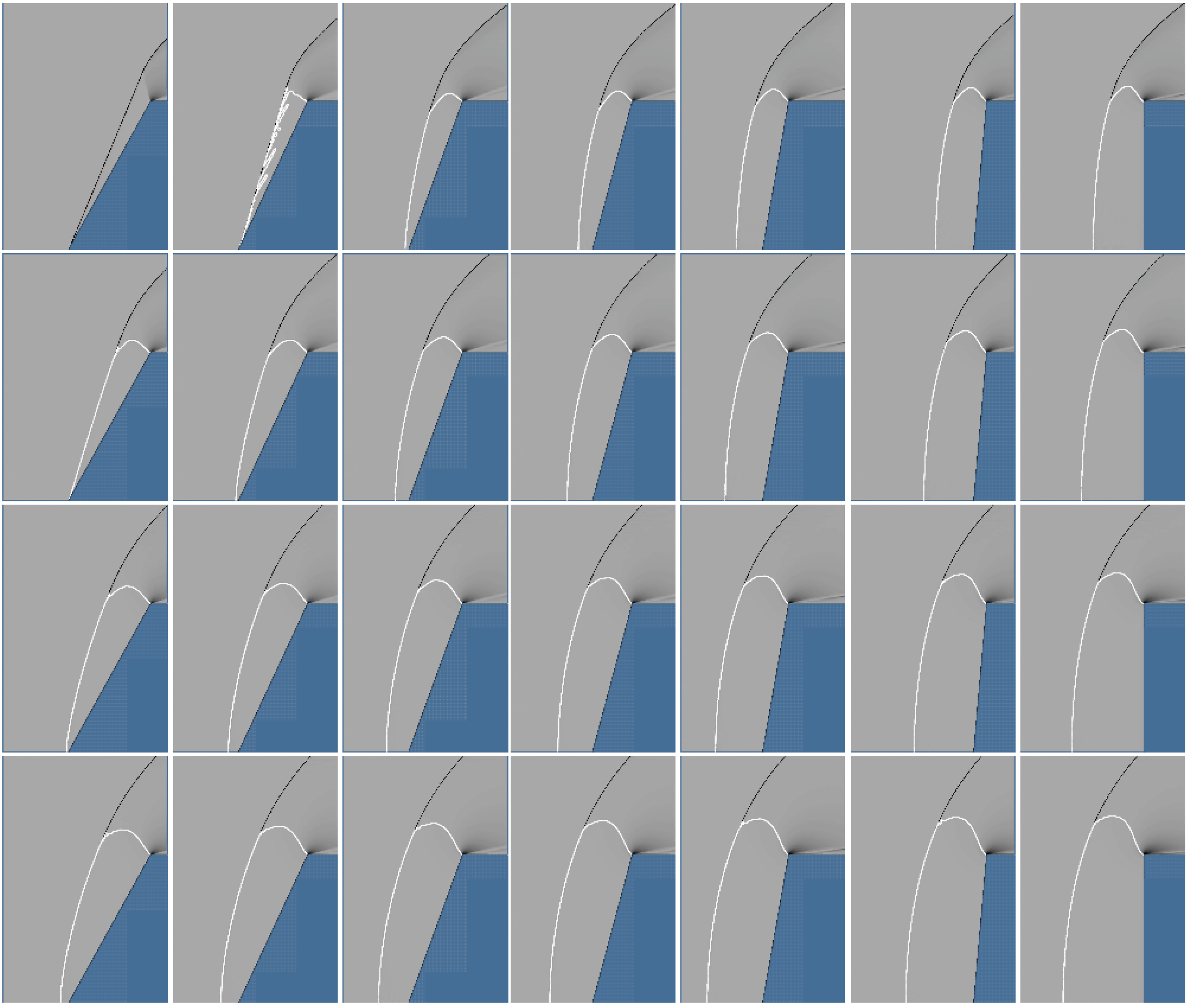
As indicated at the end of the last section, the parameter space was explored by computing the flow over cones using the Euler equations. Details about the computational technique are given in the Appendix. An example of the results is presented in figure 6 for the case of
 $M_{\infty }=5$
. Similar results were also obtained for
 $M_{\infty }=3.5$
and 10. Plotting the dimensionless shock stand-off distance against
 $\unicode[STIX]{x1D700}$
in the case
 $\unicode[STIX]{x1D703}=90^{\circ }$
(flat-faced cylinder), i.e. for
 $\unicode[STIX]{x1D702}=1$
, where
 $f(\unicode[STIX]{x1D702})=f(1)$
is a constant, provides a partial test of the hypothesis for the function
 $g(\unicode[STIX]{x1D700})$
.
Pseudo-schlieren images of flow over cones at
 $M_{\infty }=5$
. In columns, left to right,
 $\unicode[STIX]{x1D703}=$
61, 65, 70, 75, 80, 85 and 90 degrees. In rows, top to bottom,
 $\unicode[STIX]{x1D6FE}=$
1.1, 1.2, 1.3 and 1.4.

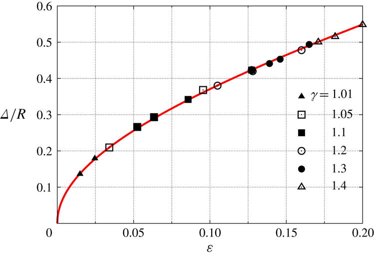
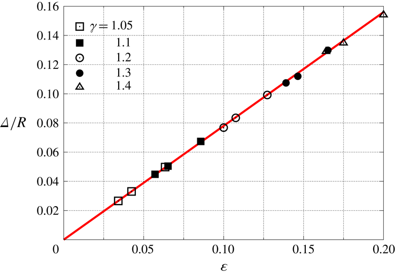
Dimensionless shock stand-off distance for
 $\unicode[STIX]{x1D703}=\unicode[STIX]{x03C0}/2$
from computations at
 $M_{\infty }=3.5$
, 5, 7.37 and 10, and
 $\unicode[STIX]{x1D6FE}$
, ranging from 1.01 to 1.4, showing that a unique function
 $g(\unicode[STIX]{x1D700})$
exists. The curve is (4.1) multiplied by
 $f(1)=1.12$
.

This has been done in figure 7. A fit to the points in figure 7 yields the interesting result that
 $$\begin{eqnarray}g(\unicode[STIX]{x1D700})=\sqrt{\unicode[STIX]{x1D700}}(1+\unicode[STIX]{x1D700}/2).\end{eqnarray}$$
Interesting, first, because it confirms part of our hypothesis, and second, because the leading term is the square root of
 $\unicode[STIX]{x1D700}$
as distinct from the case of a sphere. Results for a sphere are presented in figure 9 for completeness. We shall return to this difference later.
Although
 $g(\unicode[STIX]{x1D700})$
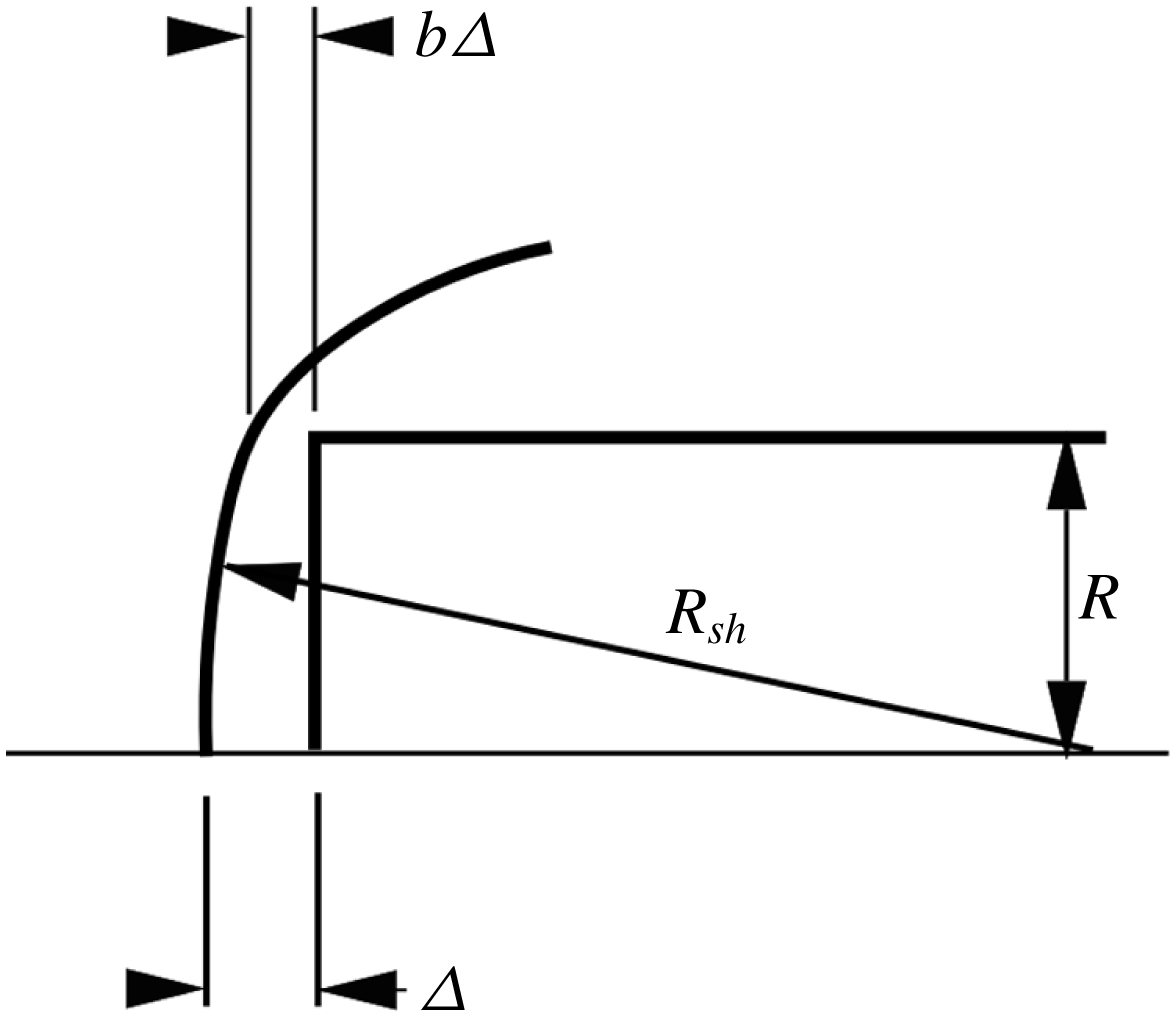
was obtained in an empirical manner, the power of the leading term may be seen to be plausible as follows: let the shock be located a distance
 $b(\unicode[STIX]{x1D700})\unicode[STIX]{x1D6E5}$
upstream of the shoulder of the
 $90^{\circ }$
cone, see figure 8. All the mass flux that crosses the shock up to the radius
 $R$
has to flow through this gap. Therefore
 $b(\unicode[STIX]{x1D700})$
cannot go to zero as
 $\unicode[STIX]{x1D700}\rightarrow 0$
. The leading term in an expansion of
 $b(\unicode[STIX]{x1D700})$
must therefore be a constant. Pythagoras’ theorem may be used to obtain the shock radius of curvature on the stagnation line,
 $R_{sh}$
approximately as
 $R^{2}/[2(1-b)\unicode[STIX]{x1D6E5}]$
. The control volume argument of Wen & Hornung (Reference Wen and Hornung1995) (see also Stulov Reference Stulov1969) shows that, for axisymmetric flow over any convex body, the leading term in
 $\unicode[STIX]{x1D6E5}/R_{sh}$
is proportional to
 $\unicode[STIX]{x1D700}$
. Since the leading term in
 $b$
is a constant, substituting for
 $R_{sh}$
shows that the leading term in
 $\unicode[STIX]{x1D6E5}/R$
is proportional to
 $\sqrt{\unicode[STIX]{x1D700}}$
.
While we were revising the manuscript, A. Tumin (2019, private communication) pointed out to us a sentence in Krasnov (Reference Krasnov1970) in which he states in the context of the
 $90^{\circ }$
cone: ‘An empirical form for the relative detachment distance can be established from experimental data in the form
 $$\begin{eqnarray}\frac{\unicode[STIX]{x1D6E5}}{R}=1.03\sqrt{\frac{\unicode[STIX]{x1D700}}{1-\unicode[STIX]{x1D700}}}\text{'}.\end{eqnarray}$$
It is interesting that, in the range of
 $\unicode[STIX]{x1D700}$
of interest here, the functional form of this expression is almost identical to
 $g(\unicode[STIX]{x1D700})$
, though the constant 1.03 differs from our value 1.12 significantly.
Assuming the shock to be a distance
 $b\unicode[STIX]{x1D6E5}$
upstream of the shoulder of a flat-faced cylinder, Pythagoras’ theorem may be used to obtain
 $R_{sh}\simeq R^{2}/[2(1-b)\unicode[STIX]{x1D6E5}]$
.

Dimensionless shock stand-off distance on a sphere at
 $M_{\infty }=5$
, 7.37 and 10,
 $\unicode[STIX]{x1D6FE}=1.05$
, 1.1, 1.2, 1.3 and 1.4, illustrating the linear behaviour. The straight line is (2.3).

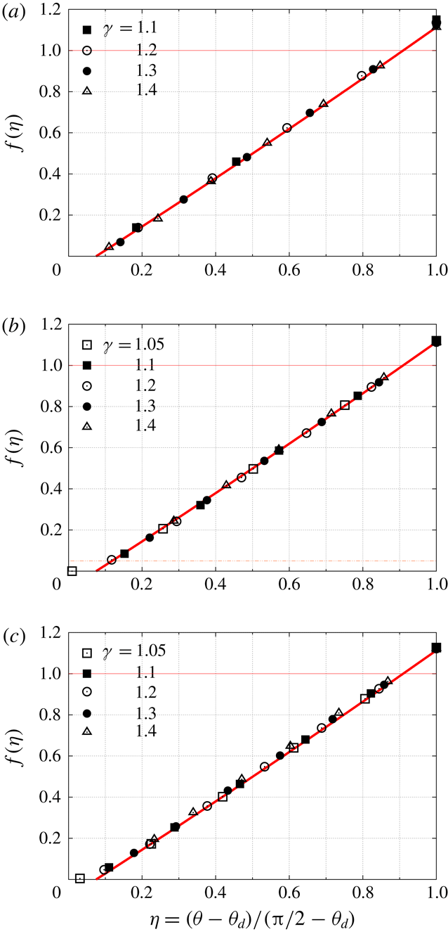
In order to test the second part of the hypothesis, figure 10 shows plots of
 $f(\unicode[STIX]{x1D702})=\unicode[STIX]{x1D6E5}/(Rg(\unicode[STIX]{x1D700}))$
for ranges of
 $M_{\infty }$
and
 $\unicode[STIX]{x1D6FE}$
. It is clear from these that, to an excellent approximation, the second part of the hypothesis is also confirmed, yielding the functional form to be
 $$\begin{eqnarray}f(\unicode[STIX]{x1D702})=1.15(\unicode[STIX]{x1D702}-0.075)+0.06(\unicode[STIX]{x1D702}-0.075)^{2}.\end{eqnarray}$$
Dimensionless shock stand-off distance divided by
 $g(\unicode[STIX]{x1D700})$
for
 $\unicode[STIX]{x1D703}=61$
, 65, 70, 75, 80, 85 and
 $90^{\circ }$
,
 $\unicode[STIX]{x1D6FE}=1.05$
, 1.1, 1.2, 1.3 and 1.4, at
 $M_{\infty }=10$
top, 5 middle and 3.5 bottom, plotted against
 $\unicode[STIX]{x1D702}$
. The curve is (4.2), and is the same in all three of the figures, illustrating that a unique function
 $f(\unicode[STIX]{x1D702})$
exists that covers all these cases.

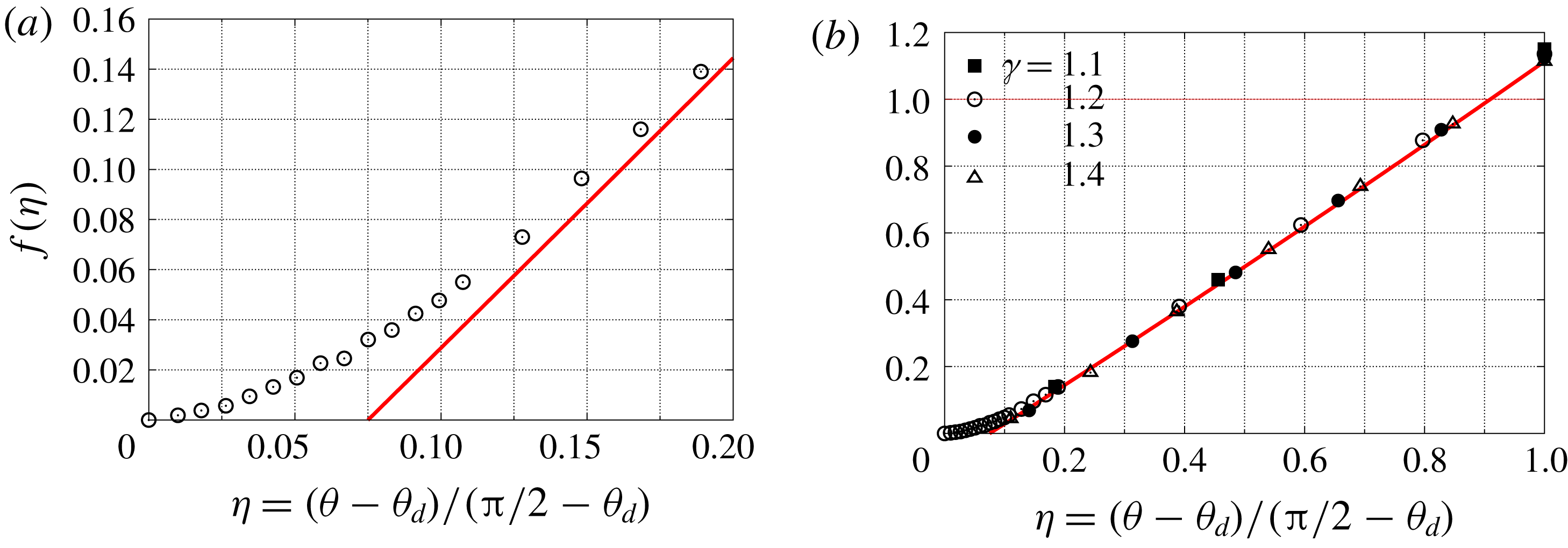
This result has the alarming feature that there seems to exist a small range
 $\unicode[STIX]{x1D702}<0.075$
, where the shock is attached. Since an attached shock cannot exist at
 $\unicode[STIX]{x1D703}>\unicode[STIX]{x1D703}_{d}$
, it is necessary to investigate this further. To this end, a series of computations were made with greatly increased resolution for the case of
 $M_{\infty }=10$
and
 $\unicode[STIX]{x1D6FE}=1.2$
. The results are shown in figure 11. This shows that, as
 $\unicode[STIX]{x1D702}$
increases from 0, the shock stand-off distance first increases very slowly, before taking off around
 $\unicode[STIX]{x1D702}=0.075$
. It should be pointed out that in order to obtain consistent measurements of
 $\unicode[STIX]{x1D6E5}$
it was measured from the well-defined tip of the cone to the thin sonic line within the shock. In this manner some degree of independence of the measurement from resolution is achieved.
(a) Behaviour of the solution near
 $\unicode[STIX]{x1D702}=0$
from more highly resolved computations,
 $M_{\infty }=10$
,
 $\unicode[STIX]{x1D6FE}=1.2$
. (b) Plot of the same results together with other
 $M_{\infty }=10$
points. Note the difference in the scales of the coordinates between (a) and (b). In both panels the curve is (4.2).

The confirmation of the hypothesis and the functional form of
 $g$
and
 $f$
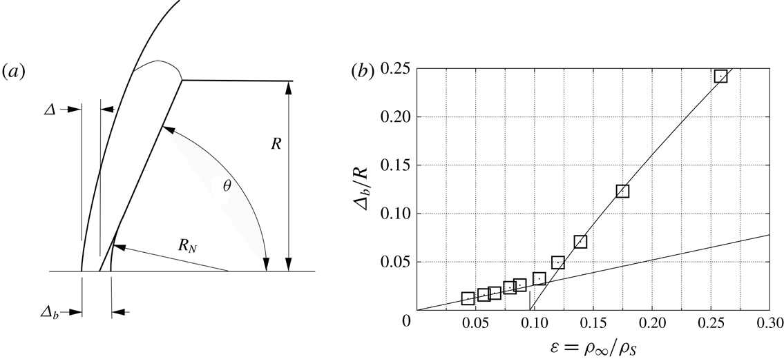
now permit us to replace the somewhat arbitrary cone behaviour line in figure 3 with an analytical one. However, since the analytical form is based on measurements from the sharp-cone tip, and the points in figure 3 represent measurements from the spherical nose, a correction needs to be applied. Figure 12 illustrates the basis of this correction and the quality of the resulting analytical cone behaviour line.
(a) Illustrating the need for the correction
 $R_{N}(1/\sin \unicode[STIX]{x1D703}-1)$
in comparing measurements of
 $\unicode[STIX]{x1D6E5}$
from spherical nose and sharp tip. (b) A replot of figure 3 with the cone behaviour curve derived from the analytical result, equation (4.2), with this correction.

Returning to the difference in the
 $\unicode[STIX]{x1D700}$
-dependence of the shock stand-off distance between the sphere and the
 $90^{\circ }$
cone,
 $$\begin{eqnarray}\frac{\unicode[STIX]{x1D6E5}}{R}=0.78\unicode[STIX]{x1D700}\quad \text{and}\quad \frac{\unicode[STIX]{x1D6E5}}{R}=1.12\sqrt{\unicode[STIX]{x1D700}}(1+\unicode[STIX]{x1D700}/2).\end{eqnarray}$$
Note that, in the range of
 $\unicode[STIX]{x1D700}$
of interest here, the latter is almost indistinguishable from the functional form
 $\sqrt{\unicode[STIX]{x1D700}(1+\unicode[STIX]{x1D700})}$
. Thus, if a way in which a smooth transition between the sphere and the
 $90^{\circ }$
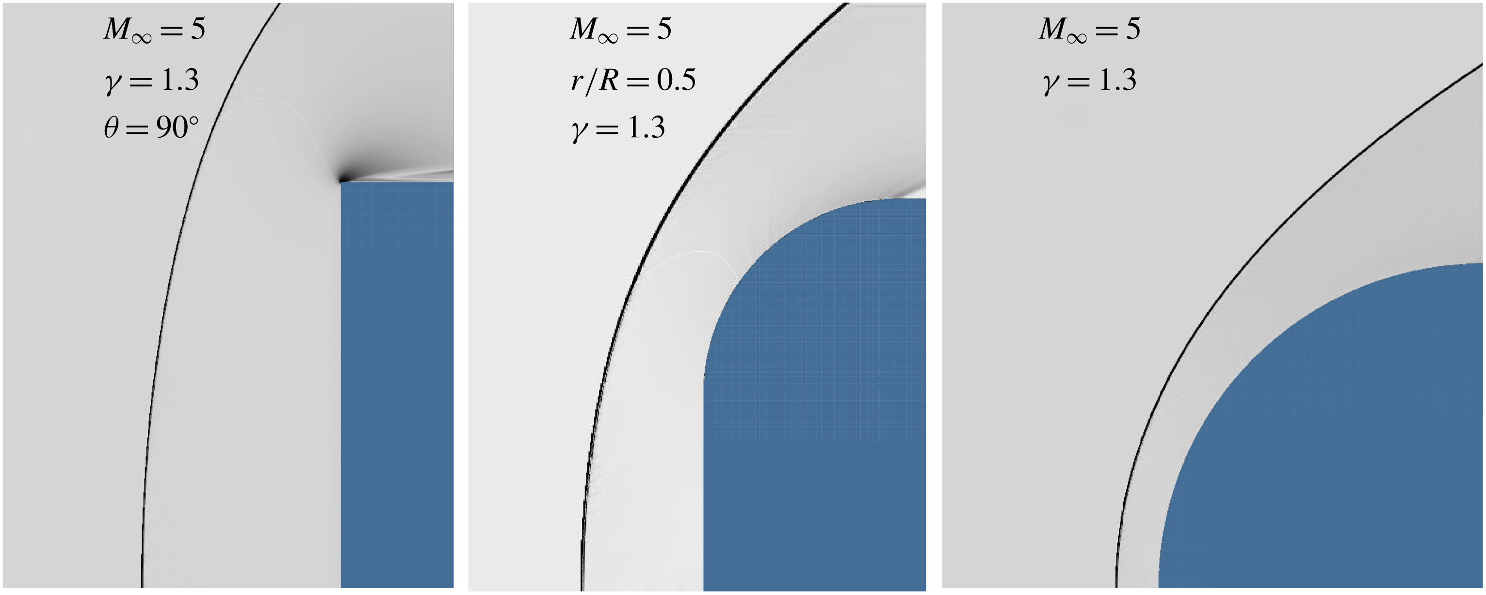
cone can be found such that the parameter describing it turns the value 1 in this expression to zero for the sphere, the difference in the functional forms for the two bodies might be accommodated. Such a smooth transition can be achieved by rounding the cone shoulder with a radius
 $r$
, as shown in figure 13. (In places where real capsule shapes are discussed, such as in § 1.1 and in Part 2,
 $r$
is denoted by
 $R_{S}$
).
Flow over a
 $90^{\circ }$
cone,
 $r/R=0$
, a
 $90^{\circ }$
cone with rounded shoulder,
 $r/R=0.5$
, and a sphere,
 $r/R=1$
, at
 $M_{\infty }=5$
,
 $\unicode[STIX]{x1D6FE}=1.3$
, showing the smooth transition controlled by the parameter
 $r/R$
.

A number of computations with
 $r/R$
ranging from 0 to 1,
 $M_{\infty }=5$
and 10,
 $\unicode[STIX]{x1D6FE}=1.1$
, 1.2, 1.3 and 1.4 gave results that were well fitted by
 $$\begin{eqnarray}\frac{\unicode[STIX]{x1D6E5}}{R}=1.12(1-0.301r/R)\sqrt{\unicode[STIX]{x1D700}(1-r/R+\unicode[STIX]{x1D700})}.\end{eqnarray}$$
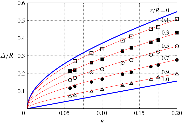
This is shown in figure 14. We note here that the case
 $r/R=0.1$
is relevant to the shapes considered in Part 2.
Results from computations of flow at
 $M_{\infty }=5$
and 10,
 $\unicode[STIX]{x1D6FE}=1.1$
, 1.2, 1.3 and 1.4,
 $r/R=0.1$
, 0.3, 0.5, 0.7 and 0.9 compared with (4.4). Also shown as thick lines are the limits for the
 $90^{\circ }$
cone (
 $r/R=0$
, equation (4.1) multiplied by
 $f(1)=1.12$
) and the sphere (
 $r/R=1$
, equation (2.3)).

4.2 Drag coefficient
If one dimensionless quantity follows the functional form of (3.5), then so should others. We therefore expect that the pressure drag coefficient
 $$\begin{eqnarray}C_{D}=\frac{2D}{\unicode[STIX]{x1D6FE}p_{\infty }M_{\infty }^{2}\unicode[STIX]{x03C0}R^{2}}\end{eqnarray}$$
behaves like
 $$\begin{eqnarray}C_{D}=g_{1}(\unicode[STIX]{x1D700})f_{1}(\unicode[STIX]{x1D702}).\end{eqnarray}$$
Here,
 $p_{\infty }$
is the free-stream pressure and the drag force
 $$\begin{eqnarray}D=\int _{0}^{R}2\unicode[STIX]{x03C0}(p-p_{\infty })y\,\text{d}y,\end{eqnarray}$$
 $p$
being the surface pressure and
 $y$
the distance measured normal to the cone axis. In the following we use only the forebody pressure for
 $p$
, so that our definition is equivalent to having a uniform base pressure equal to
 $p_{\infty }$
.
In order to determine whether a unique function
 $g_{1}(\unicode[STIX]{x1D700})$
exists, the drag coefficient of flow over
 $90^{\circ }$
cones is plotted in figure 15 for ranges of
 $M_{\infty }$
and
 $\unicode[STIX]{x1D6FE}$
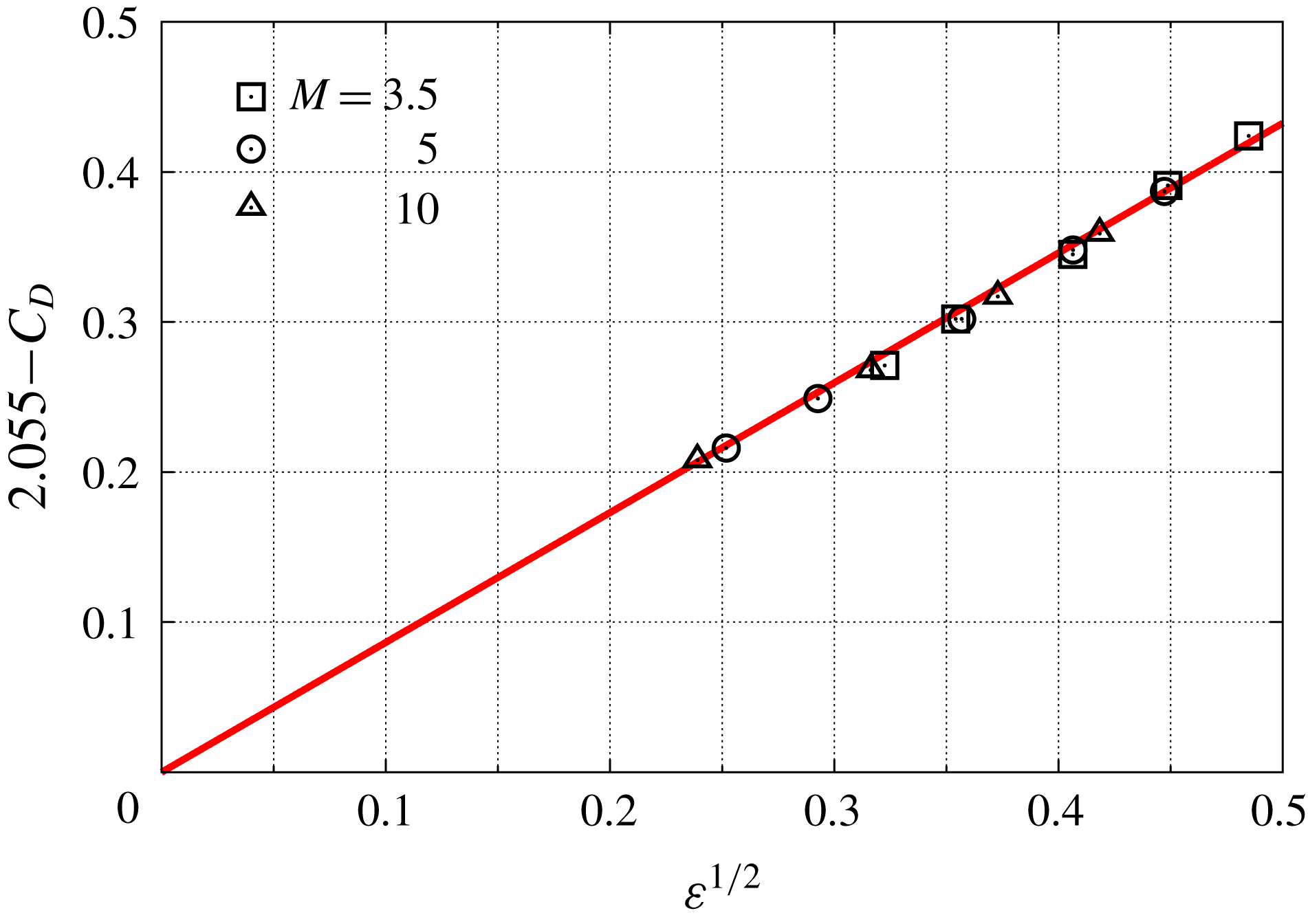
. This shows that such a function does indeed exist and is very well approximated by
 $$\begin{eqnarray}g_{1}(\unicode[STIX]{x1D700})=2.055-0.865\sqrt{\unicode[STIX]{x1D700}}.\end{eqnarray}$$
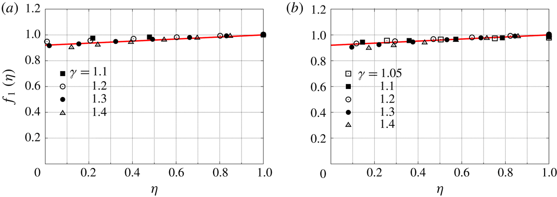
The uniqueness of the function
 $f_{1}(\unicode[STIX]{x1D702})$
is not as convincing as that of
 $f(\unicode[STIX]{x1D702})$
is in the case of
 $\unicode[STIX]{x1D6E5}/R$
, as may be seen in figure 16. However, the dependence of
 $C_{D}$
on
 $\unicode[STIX]{x1D702}$
is quite weak. An approximation to the results is
 $$\begin{eqnarray}f_{1}(\unicode[STIX]{x1D702})=0.92+0.08\unicode[STIX]{x1D702}.\end{eqnarray}$$
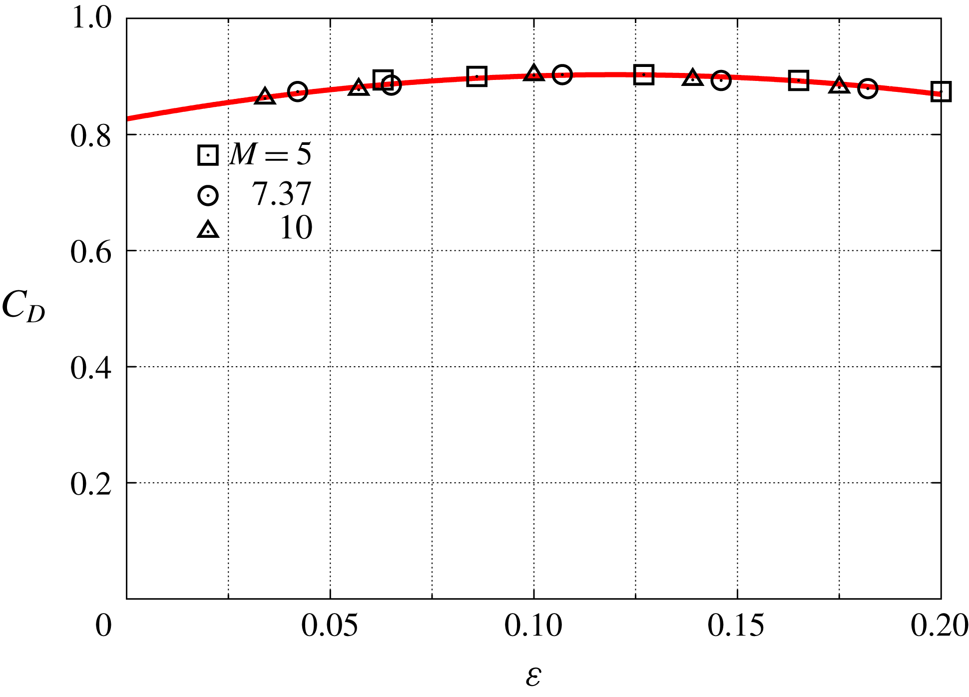
The drag coefficient of a sphere should also be a function only of
 $\unicode[STIX]{x1D700}$
. The plot in figure 17 shows that this is the case, and that
 $$\begin{eqnarray}C_{D}=0.903-5.2(\unicode[STIX]{x1D700}-0.12)^{2}.\end{eqnarray}$$
Plot of
 $2.055-C_{D}$
against
 $\sqrt{\unicode[STIX]{x1D700}}$
for flow over a
 $90^{\circ }$
cone at
 $M_{\infty }=3.5$
, 5 and 10, and
 $\unicode[STIX]{x1D6FE}=1.05$
, 1.1, 1.2, 1.3 and 1.4. The straight line corresponds to (4.8).

Test for the function
 $f_{1}(\unicode[STIX]{x1D702})$
using flows at
 $\unicode[STIX]{x1D703}=61$
, 65, 70, 75, 80, 85 and
 $90^{\circ }$
, and
 $\unicode[STIX]{x1D6FE}=1.05$
, 1.1, 1.2, 1.3 and 1.4. (a)
 $M_{\infty }=10$
, (b)
 $M_{\infty }=5$
. In both panels the line is (4.9).

Drag coefficient of a sphere at
 $M_{\infty }=5$
, 7.37 and 10, and
 $\unicode[STIX]{x1D6FE}=1.05$
, 1.1, 1.2, 1.3 and 1.4. The curve is (4.10).

5 Cone with
 $r/R=0.1$

All of the results presented in § 4 for the cone with sharp shoulder are repeated for the case of practical interest in Part 2, where the shoulder is rounded to
 $r/R=0.1$
. The results confirm the hypothesis equally convincingly in that case and the results are that
 $$\begin{eqnarray}\frac{\unicode[STIX]{x1D6E5}}{R}=1.049\sqrt{\unicode[STIX]{x1D700}}(1+0.55\unicode[STIX]{x1D700})[(\unicode[STIX]{x1D702}-0.075)+0.032(\unicode[STIX]{x1D702}-0.075)^{2}]\end{eqnarray}$$
and
 $$\begin{eqnarray}C_{D}=(1.9-0.94\sqrt{\unicode[STIX]{x1D700}})(0.95+0.05\unicode[STIX]{x1D702}).\end{eqnarray}$$
6 High-enthalpy real-gas effects
All the work in Part 1 assumes perfect-gas behaviour. However, as has been shown e.g. by Stulov (Reference Stulov1969) and by Wen & Hornung (Reference Wen and Hornung1995), replacing the normal-shock density ratio by the ratio of the average density along the stagnation streamline to the free-stream density permits such results to be carried over to the high-enthalpy real-gas case. Although Wen & Hornung (Reference Wen and Hornung1995) have only shown this to apply to flow over spheres, Stulov (Reference Stulov1969) proposes that it also applies to other blunt bodies. It is interesting that, because Wen & Hornung (Reference Wen and Hornung1995) use the average density, the constant in their relation between dimensionless stand-off distance and density ratio for a sphere is not 0.78 but 0.82. This is consistent with the fact that the average density along the stagnation streamline for perfect-gas flow over a sphere with
 $\unicode[STIX]{x1D6FE}=1.4$
is 5 % higher than the shock density.
7 Conclusions
A discussion of the extensive literature on the subject of blunted-cone capsules is presented. Sphere and cone behaviour of hypersonic flow over a spherically blunted cone are discussed and elucidated by considering the two elements: the sphere and the sharp cone. The inflection point in the shock shape for sphere behaviour is explained. A novel approach is applied in which a large number of computational results are used to discover analytical relationships that fit in with hypersonic similarity theory. Analytical functions of two independent variables (
 $\unicode[STIX]{x1D700},\unicode[STIX]{x1D702}$
) are found, in place of unknown functions of three independent variables (
 $M_{\infty },\unicode[STIX]{x1D6FE},\unicode[STIX]{x1D703}$
) for the shock wave stand-off distance and the drag coefficient. An analytical form is found for the shock stand-off distance in the transition from the
 $90^{\circ }$
cone to the sphere. This work is repeated for the case of the cone with 10 % rounded shoulder that is relevant to Part 2. The relevance of these perfect-gas results to high-enthalpy real-gas situations is explained.
Appendix
The software system Amrita, constructed by Quirk (Reference Quirk1998), was used. A detailed description of the features and phenomena encountered with some of the algorithms used for Riemann solvers, including the one used here, has also been given by Quirk (Reference Quirk1994). An example of a test of the software against experiment may be found in Quirk & Karni (Reference Quirk and Karni1996).
Amrita is a system that automates and packages computational tasks in such a way that the packages can be combined (dynamically linked) according to instructions written in a high-level scripting language. The present application uses features of Amrita that include the automatic construction of the Euler solver, documentation of the code, adaptive mesh refinement according to simply chosen criteria and scripting-language-driven computation, archiving and post-processing of the results. The automation of the assembly and sequencing of the tasks makes for dramatically reduced possibility of hidden errors. It also makes computational investigations transparent and testable by others. The ability to change one package at a time, without changing the rest of the scheme, facilitates detection of sources of error. In most of the work, the Euler solver generated was an operator-split scheme with HLLE flux (after Harten, Lax & van Leer (Reference Harten, Lax and van Leer1983) and Einfeldt (Reference Einfeldt1988)) and kappa-MUSCL reconstruction. In some cases with
 $\unicode[STIX]{x1D6FE}$
close to 1, the carbuncle problem arose, and the more robust equilibrium flux method of Pullin (Reference Pullin1980) was used. The (
 $x,y$
) plane was discretized by a Cartesian grid of
 $600\times 600$
coarse–grid cells that were adaptively refined by a factor of 3 to make an effective grid of
 $1800\times 1800$
cells. The criterion for adaptation was a chosen threshold of the magnitude of the density gradient. Solid boundaries are represented by a level set defined as the smallest distance of a field point from the solid boundary. In the case of the more highly resolved computations that were used to clear up the situation at small
 $\unicode[STIX]{x1D702}$
, a further adaptive refinement factor of 3 was applied to both coordinates. The grey shading of the visualizations is a monotonic function of the magnitude of the density gradient.