
1. Introduction
Many micro-organisms self-propel through liquid by continuously rotating a helical or screw-like filament. A prime example is Escherichia coli. In order to swim, it bundles its flagella in a single helical tail and rotates the bundle to propel itself forward. The prominence of this swimming strategy in the microscopic realm derives from the unique properties of highly viscous flows: owing to the linearity and time reversibility of the Stokes equation, a time-reversible sequence of mechanical deformations of a swimmer's body cannot induce a net displacement (Purcell Reference Purcell1977). Continuous rotation of a helical tail evades this so-called ‘scallop theorem’. In terms of mechanical forces, this swimming strategy exploits the anisotropy of the Stokes drag force on a moving rod; the entire tail can be regard as made up of rod-like segments, and the anisotropic drag, when integrated over the helix contour, yields a net propulsive force, i.e. thrust (Lauga & Powers Reference Lauga and Powers2009).
Recently, inspired by nature, and facilitated by advances in colloid fabrication methods, a wide range of artificial microswimmers has been developed. Initially, manufacturing capabilities limited those to simple shapes, e.g. spheres, spheroids and rods. However, more recently, complex and non-axisymmetric shapes have come into focus (Gibbs Reference Gibbs2020). For instance, Gibbs and Fischer showcase helical microdrills that consist of a spherical ‘head’ and helical ‘tail’ (Gibbs & Fischer Reference Gibbs and Fischer2015). On the surface, the design resembles the aforementioned E. coli. However, this design is a self-phoretic particle: it is covered by a catalyst, and when immersed in a solution containing molecular ‘fuel’, induces and sustains gradients of the various molecular species involved in the reaction. The chemical gradients, in conjunction with the molecular forces of interaction between the molecules and the particle surface, drive fluid flow in the vicinity of the particle surface, leading to directed motion (Anderson Reference Anderson1989). Accordingly, the superficial similarity between E. coli, a mechanical swimmer, and self-phoretic helical swimmers may not hold up upon more detailed investigation. For instance, it is not obvious whether self-phoretic helices would exhibit any significant rotation around the helix axis, or display circular trajectories when in the vicinity of a solid boundary, a well-known behaviour of E. coli (Lauga et al. Reference Lauga, Luzio, Whitesides and Stone2006; Berke et al. Reference Berke, Turner, Berg and Lauga2008). Furthermore, the optimal geometry of a helical self-phoretic swimmer for self-propulsion is of obvious interest, and may not be identical to that of a mechanical swimmer. As another example, we note that enhancing the screw axis rotation of a self-phoretic helix would enhance its function as a microdrill. However, rotations with respect to the other body axes would hinder this function. More generally, rotary micromotors and nanomotors are envisioned as key elements of future active colloidal machines (Kim et al. Reference Kim, Guo, Liang, Zhu and Fan2016; Aubret et al. Reference Aubret, Youssef, Sacanna and Palacci2018); being able to control their motion (e.g. by restricting rotation to only one body-fixed axis) by design would boost development of these applications.
The aim of this work is develop a framework to study implications of the helical geometry for self-phoretic swimmers, and their possibilities for a wide range of applications, e.g. in lab-on-a-chip devices or for targeted drug delivery. We start by introducing the mathematical description of the particle shape in § 2.1. We then outline the physical model and governing equations in § 2.2. In § 2.3, we specify activity profiles, i.e. distributions of catalytic activity over the particle surface. We detail three model activity profiles that are relevant to current experiments. Before presenting our results, we outline our numerical method in § 2.5. In the results (§ 3), we discuss the hydrodynamic resistance tensor in § 3.1, and then the concentration field and the particle velocities for three different activity profiles in §§ 3.2–3.4. Finally, we provide a novel and detailed development of slender body theory (SBT) for the concentration in § 3.5.
On this path, the hydrodynamic resistance tensor turns out to be a highly important quantity. Calculation of the hydrodynamic resistance tensor for a helix is a classical problem in low Reynolds number hydrodynamics that sparks interest in its own right (Gray & Handcock Reference Gray and Handcock1955; Johnson Reference Johnson1980; Purcell Reference Purcell1997; Rodenborn et al. Reference Rodenborn, Chen, Swinney, Liu and Zhang2013; Palusa et al. Reference Palusa, de Graaf, Brown and Morozov2018; du Roure et al. Reference du Roure, Lindner, Nazockdast and Shelley2019). Moreover, it has additional relevance for application to magnetically driven helical swimmers (Ghosh & Fischer Reference Ghosh and Fischer2009; Man & Lauga Reference Man and Lauga2013; Peyer et al. Reference Peyer, Tottori, Qiu, Zhang and Nelson2013; Bianchi et al. Reference Bianchi, Sosa, Vizsnyiczai and Di Leonardo2020; Mirzae et al. Reference Mirzae, Rubinstein, Morozov and Leshansky2020). With our numerical implementation of the boundary element method (BEM), we obtain good agreement with the experimental estimates of resistance tensor components obtained by Purcell (Reference Purcell1997) and corresponding numerical calculations from Cortez, Fauci & Medovikov (Reference Cortez, Fauci and Medovikov2005), validating our approach. Moreover, we find that SBT, which resolves hydrodynamic interactions between particle segments – but not the finite thickness of the particle – exhibits excellent agreement with detailed calculations obtained with the BEM. In contrast, resistive force theory, which neglects hydrodynamic interactions, performs poorly (Rodenborn et al. Reference Rodenborn, Chen, Swinney, Liu and Zhang2013). These findings have implications for the study of helix sedimentation dynamics (Palusa et al. Reference Palusa, de Graaf, Brown and Morozov2018).
Regarding the concentration, our numerical calculations and extended SBT show that, in general, there will be circumferential spatial variations (i.e. variations circling around the contour tangent vector) in the vicinity of the particle surface. Notably, these variations are absent for simple geometries, e.g. spheres and spheroids with axisymmetric patterning, and they contribute to particle motion. Depending on the helix parameters (pitch, catalyst coverage, etc.), these variations can become negligible compared with, or dominate over, the tangential variations. In the latter case, one can observe significant motion perpendicular to the helix screw axis. This qualitative dependence on the helix parameters allows one to choose between a wide range of possible trajectories by changing only one or two aspects of the helix.
2. Theory
2.1. Particle geometry
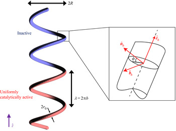
We consider a solid particle that has the shape of a cylindrical tube bent into a helical contour (figure 1). The tube radius is  $r_0$, the radius of the tube centreline around the helix axis is
 $R$, the helix pitch is
 $\lambda$, the end-to-end distance is
 $L$ and the total contour length of the helix is
 $\mathscr {L}$. The two ends of the particle are terminated by hemispherical caps with radius
 $r_0$. The centreline of the tube (between the two caps) is described by a space curve
 $\boldsymbol {x}_h(t)$ parameterized by
 $t$
 \begin{equation} \left.\begin{array}{c@{}} x_h = R \cos t \\ y_h = R \sin t \\ z_h = bt \end{array}\right\}, \end{equation}
where  $2 {\rm \pi}b = \lambda$. The helix has
 $N$ turns, so that
 ${L} = N \lambda$,
 $\mathscr {L} = N \sqrt {\lambda ^{2} + (2 {\rm \pi}R)^{2}}$ and
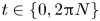 $t \in \{0, 2 {\rm \pi}N\}$. The surface of the tube (between the end caps) is described by
 \begin{equation} \left.\begin{array}{c@{}} \displaystyle x_s = R \cos t - r_0 \cos t \cos \phi + \dfrac{r_0 b}{\sqrt{R^{2} + b^{2}}} \sin t \sin \phi \\ \displaystyle y_s = R \sin t - r_0 \sin t \cos \phi - \dfrac{r_0 b}{\sqrt{R^{2} + b^{2}}} \cos t \cos \phi \\ \displaystyle z_s = bt + \dfrac{r_0 b}{\sqrt{R^{2} + b^{2}}} \cos \phi \end{array}\right\}, \end{equation}
where  $\phi \in \{0, 2 {\rm \pi}\}$ is an angle that describes position on the circular cross-section of the tube surface centred at position
 $t$ on the centreline. At any point
 $t$ on the helix, the tangent vector
 $\hat {\boldsymbol {t}}_h \equiv {\partial \boldsymbol {x}_h}/{\partial t} / |{\partial \boldsymbol {x}_h}/{\partial t}|$, normal vector
 $\hat {\boldsymbol {n}}_{h} \equiv {\partial \hat {\boldsymbol {t}}_h}/{\partial t} / |{\partial \hat {\boldsymbol {t}}_h}/{\partial t}|$ and binormal vector
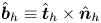 $\hat {\boldsymbol {b}}_h \equiv \hat {\boldsymbol {t}}_h \times \hat {\boldsymbol {n}}_h$ define three orthogonal vectors, where
 $\hat {\boldsymbol {t}}_h = (- {{R} \sin t}/{\sqrt {{R}^{2} + b^{2}}}, {{R} \cos t}/{\sqrt {{R}^{2} + b^{2}}}, {b}/{\sqrt {{R}^{2} + b^{2}}} )$,
 $\hat {\boldsymbol {n}}_h = (- \cos t, -\sin t, 0)$ and
 $\hat {\boldsymbol {b}}_h = ( {b \sin t}/{\sqrt {{R}^{2} + b^{2}}}, -{b \cos t}/{\sqrt {{R}^{2} + b^{2}}}, {{R}}/{\sqrt {{R}^{2} + b^{2}}} )$. Accordingly, for a point on the surface of the tube,
 $\phi = 0^{\circ }$ if the point is displaced from the tube centreline along the local normal
 $\hat {\boldsymbol {n}}_h$, and
 $\phi = 90^{\circ }$ if it is displaced from the centreline along the local binormal
 $\hat {\boldsymbol {b}}_h$. Note that the local surface normal
 $\hat {\boldsymbol {n}}_h$ always points towards the axis of the helix, entailing that a point on the particle surface with
 $\phi = 0^{\circ }$ is in the interior space.
Schematic illustration of the particle geometry. The particle consists of a solid ‘tube’ with a helical contour and circular cross-section, plus two solid hemispherical endcaps. Here, we label the contour radius  $R$, the helix pitch
 $\lambda$, the tube radius
 $r_0$, the local tangent vector
 $\hat {\boldsymbol {t}}_h$, the local surface normal
 $\hat {\boldsymbol {n}}_h$ and the local surface binormal
 $\hat {\boldsymbol {b}}_h$. For a given point on the tube centreline, the angle
 $\phi$ defines a point on the tube surface. In this example, the particle has a ‘lengthwise Janus’ catalytic activity profile.

For the following analysis, we also find it useful to define the tangential position  $s \in [-1,1]$ along the centreline of the cylindrical tube, where
 $s = -1$ corresponds to the centre of the base of one hemispherical endcap,
 $s = 1$ to the centre of the base of the other hemispherical endcap and
 $s = 0$ to the midpoint of the contour. Additionally, all geometric quantities will be specified in terms of a characteristic length scale
 $L_0 \sim R$.
2.2. Physical model and governing equations
We consider a stationary reference frame in which the instantaneous position of the geometric centroid of the helix is  $\boldsymbol {x}_p = (x_p, y_p, z_p)$. The helix is immersed in a liquid solution containing reactant (‘fuel’) molecules, and part of the surface of the helix catalyses the decomposition of the reactant, producing a reaction product that has a number density field
 $c(\boldsymbol {x})$ (hereafter called the concentration field), where
 $\boldsymbol {x}$ is a position in the solution. We assume that the characteristic time scale for diffusion of the reactant is much smaller than the characteristic time scale for particle motion. Therefore, the concentration field can be regarded as quasi-static, and it satisfies the Laplace equation
 $\nabla ^{2} c = 0$. The concentration field is subject to the boundary conditions
 $c(|\boldsymbol {x}| \rightarrow \infty ) = 0$ and
 $-D [\hat {\boldsymbol {n}} \boldsymbol {\cdot } \boldsymbol {\nabla } c] = \kappa j(\boldsymbol {x}_s)$ on the particle surface. Here,
 $D$ is the diffusion coefficient of the product molecules,
 $\kappa$ is a characteristic rate of solute production per unit area,
 $\boldsymbol {x}_s$ is a position on the particle surface and
 $\hat {\boldsymbol {n}}$ is a unit vector locally normal to the particle surface. The normal is defined to point into the fluid. (Note that the surface normal
 $\hat {\boldsymbol {n}}$ is distinct from the space curve normal
 $\hat {\boldsymbol {n}}_h$ introduced in the previous section. In particular,
 $\hat {\boldsymbol {n}} = \cos \phi \hat {\boldsymbol {n}}_h + \sin \phi \hat {\boldsymbol {b}}_h$ over the tube surface.) The function
 $j(\boldsymbol {x}_s)$ is dimensionless, and describes the distribution of catalytic activity over the particle surface. For simplicity, we have assumed zeroth-order kinetics, i.e. the activity has no dependence on the product concentration
 $c(\boldsymbol {x})$.
The above problem for  $c(\boldsymbol {x})$ can be solved numerically, using the BEM. Once
 $c(\boldsymbol {x})$ is known, one can obtain the surface gradient
 $\nabla _s c$, where
 $\nabla _s \equiv (\boldsymbol {1} - \hat {\boldsymbol {n}}\hat {\boldsymbol {n}}) \boldsymbol {\cdot } \boldsymbol {\nabla }$. Since
 $\nabla _s c$ is defined on the surface of the particle, it lies within a plane that is locally tangent to the tube surface and has normal
 $\hat {\boldsymbol {n}}$. Conceptually, we can decompose
 $\nabla _s c$ into a tangential component,
 $(\hat {\boldsymbol {t}}_h \boldsymbol {\cdot } \nabla _s c) \hat {\boldsymbol {t}}_h$, and a circumferential component
 $(\boldsymbol {1} - \hat {\boldsymbol {t}}_h \hat {\boldsymbol {t}}_h ) \boldsymbol {\cdot } \nabla _s c = (\hat {\boldsymbol {n}}_h \boldsymbol {\cdot } \nabla _s c) \hat {\boldsymbol {n}}_h + (\hat {\boldsymbol {b}}_h \boldsymbol {\cdot } \nabla _s c) \hat {\boldsymbol {b}}_h$. This decomposition will be useful in the subsequent analysis.
The suspending fluid is assumed to be Newtonian and governed by the Stokes equation
 \begin{equation} -\boldsymbol{\nabla} P + \mu \nabla^{2} \boldsymbol{u} = 0, \end{equation}
and incompressibility condition  $\boldsymbol {\nabla } \boldsymbol {\cdot } \boldsymbol {u} = 0$, where
 $\boldsymbol {u}(\boldsymbol {x})$ is the velocity of the fluid,
 $P(\boldsymbol {x})$ is the fluid pressure, and
 $\mu$ is the viscosity. The fluid velocity is subject to the boundary conditions
 \begin{equation} \boldsymbol{u}(\boldsymbol{x}_s) = \boldsymbol{U} + \boldsymbol{\varOmega} \times (\boldsymbol{x}_s - \boldsymbol{x}_p) + \boldsymbol{v}_s(\boldsymbol{x}_s), \end{equation}
on the surface of the helical particle, where  $\boldsymbol {U}$ and
 $\boldsymbol {\varOmega }$ are the (unknown) translational and angular velocities of the particle, as well as
 $\boldsymbol {u}(|\boldsymbol {x}| \rightarrow \infty ) = 0$. The quantity
 $\boldsymbol {v}_s$, the so-called phoretic slip velocity, is obtained as
 $\boldsymbol {v}_s = -b(\boldsymbol {x}_s) \nabla _s c$, where
 $b(\boldsymbol {x}_s)$, the so-called surface mobility, is a material dependent quantity that encodes interactions between the reactant and the particle surface (Anderson Reference Anderson1989). Finally, to close the system of equations, we specify that the particle is force free,
 \begin{equation} \int_S \boldsymbol{\sigma} \boldsymbol{\cdot} \hat{\boldsymbol{n}} \,{\textrm{d}}S = 0, \end{equation}
and torque free,
 \begin{equation} \int_S (\boldsymbol{x}_s - \boldsymbol{x}_p) \times \boldsymbol{\sigma} \boldsymbol{\cdot} \hat{\boldsymbol{n}}\, {\textrm{d}}S = 0, \end{equation}
where  $S$ indicates an integral over the particle surface.
In order to solve this problem for  $\boldsymbol {U}$ and
 $\boldsymbol {\varOmega }$, we use the Lorentz reciprocal theorem. This theorem relates two solutions to the Stokes equation with the same geometry but different boundary conditions. For an auxiliary problem
 $(j)$, we write
 \begin{equation} \int_S \boldsymbol{u} \boldsymbol{\cdot} \boldsymbol{\sigma}^{(j)} \boldsymbol{\cdot} \hat{\boldsymbol{n}}\, {\textrm{d}}S = \int_S \boldsymbol{u}^{(j)} \boldsymbol{\cdot} \boldsymbol{\sigma} \boldsymbol{\cdot} \hat{\boldsymbol{n}}\, {\textrm{d}}S, \end{equation}
where auxiliary problem  $(j)$ has the boundary conditions
 \begin{equation} \boldsymbol{u}^{(j)}(\boldsymbol{x}_s) = \boldsymbol{U}^{(j)} + \boldsymbol{\varOmega}^{(j)} \times (\boldsymbol{x}_s - \boldsymbol{x}_p), \end{equation}
and  $\boldsymbol {u}^{(j)}(|\boldsymbol {x}| \rightarrow \infty ) = 0$, i.e. the particle moves as a rigid body with no slip on the surface. We specify six auxiliary problems
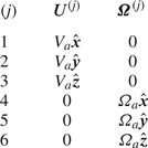
 $j \in \{1, 2,\ldots , 6\}$, with the boundary conditions for each
 $(j)$ given in table 1.
Boundary conditions for the auxiliary problem  $(j)$.

Combining (2.4), (2.7) and (2.8), we obtain
 \begin{align} &\boldsymbol{U} \boldsymbol{\cdot} \int_S \boldsymbol{\sigma}^{(j)} \boldsymbol{\cdot} \hat{\boldsymbol{n}} \, {\textrm{d}}S + \boldsymbol{\varOmega} \boldsymbol{\cdot} \int_S (\boldsymbol{x}_s - \boldsymbol{x}_p) \times \boldsymbol{\sigma}^{(j)} \boldsymbol{\cdot} \hat{\boldsymbol{n}} \, {\textrm{d}}S + \int_S \boldsymbol{v}_s(\boldsymbol{x}_s) \boldsymbol{\cdot} \boldsymbol{\sigma}^{(j)} \boldsymbol{\cdot} \hat{\boldsymbol{n}} \, {\textrm{d}}S \nonumber\\ &\quad =\boldsymbol{U}^{(j)} \boldsymbol{\cdot} \int_S \boldsymbol{\sigma} \boldsymbol{\cdot} \hat{\boldsymbol{n}} \, {\textrm{d}}S + \boldsymbol{\varOmega}^{(j)} \boldsymbol{\cdot} \int_S (\boldsymbol{x}_s- \boldsymbol{x}_p) \times \boldsymbol{\sigma} \boldsymbol{\cdot} \hat{\boldsymbol{n}} \, {\textrm{d}}S. \end{align}
According to (2.5) and (2.6), the two integrals on the right-hand side vanish. Moreover, on the left-hand side, we recognize that the integrals represent components of the hydrodynamic resistance matrix  ${\boldsymbol{\mathsf{R}}}$ (with a negative sign). Accordingly, the equation can be represented as a linear system
 \begin{equation} 6 {\rm \pi}\mu {{\boldsymbol{\mathsf{R}}}} \boldsymbol{\cdot} \begin{pmatrix} \boldsymbol{U} \\ \boldsymbol{\varOmega} \end{pmatrix} = \boldsymbol{b}, \end{equation}
where the six-component right-hand side vector  $\boldsymbol {b}$ is
 \begin{equation} b_j = \int_S \boldsymbol{v}_s(\boldsymbol{x}_s) \boldsymbol{\cdot} \boldsymbol{\sigma}^{(j)} \boldsymbol{\cdot} \hat{\boldsymbol{n}} \, {\textrm{d}}S / V^{(j)}, \end{equation}
where  $V^{(j)} = V_a$ for
 $j \in \{1, 2, 3\}$, and
 $V^{(j)} = \varOmega _a$ for
 $j \in \{4, 5, 6\}$. Note the factor of
 $6 {\rm \pi}\mu$ appears in (2.10) because of how we choose to define
 ${\boldsymbol{\mathsf{R}}}$. The various components of
 ${\boldsymbol{\mathsf{R}}}$ are proportional to, and have the same units as,
 $L_0$,
 $L_0^{2}$ or
 $L_0^{3}$. Equation (2.10) can be solved by standard methods to determine
 $\boldsymbol {U}$ and
 $\boldsymbol {\varOmega }$. Interestingly, the right-hand side vector
 $\boldsymbol {b}$ can be regarded as a generalized effective swimming force; the first three rows have units of force, and last three rows have units of torque.
Finally, from consideration of the governing equations, we determine a characteristic concentration  $c_0 \equiv \kappa L_0 / D$ and a characteristic velocity
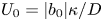 $U_0 = |b_0| \kappa / D$, where
 $|b_0|$ is a characteristic surface mobility coefficient. A characteristic force can be defined as
 $F_0 \equiv \mu U_0 L_0$. In the following, we will present quantitative results in terms of these characteristic quantities, except where noted.
2.3. Specification of catalytic activity and surface chemistry
In this work, we consider three choices of  $j(\boldsymbol {x_s})$. For all choices, we present results for uniform surface mobility, i.e.
 $b(\boldsymbol {x}_s) = b_0$, where
 $b_0 < 0$. The sign of
 $b_0$ ensures that the solute/surface interaction is repulsive, such that the particle tends to propel away from regions of high solute concentration. Although we examined the effect of a surface mobility contrast between the catalytic and inert regions, we did not find it to qualitatively change the results presented below.
2.3.1. Lengthwise Janus particle
For the ‘lengthwise Janus’ particle, like the one shown in figure 1, we choose  $j(\boldsymbol {x_s}) = \varTheta (-s)$ for a position on the surface of the cylindrical tube, where
 $\varTheta (s)$ is the Heaviside step function. Additionally, the hemispherical endcap with its base at the point
 $s = -1$ has
 $j(\boldsymbol {x_s})$ = 1, and the endcap with its base at the point
 $s = 1$ has
 $j(\boldsymbol {x_s}) = 0$. In other words, half of the particle is uniformly catalytic, and the other half is inert.
2.3.2. The  $z$-wise Janus particle

For the ‘ $z$-wise Janus’ particle, we choose
 $j(\boldsymbol {x_s}) = -(\hat {\boldsymbol {n}} \: \boldsymbol {\cdot } \hat {\boldsymbol {z}}) \varTheta (-\hat {\boldsymbol {n}} \boldsymbol {\cdot } \hat {\boldsymbol {z}})$. For this particle, the region of the surface with a negative
 $z$-component of the local surface normal
 $\hat {\boldsymbol {n}}$ is catalytically active. Additionally, over this region, the catalytic activity is proportional to the
 $z$-component of the local surface normal. This activity profile is shown in figure 8(a) for a particular choice of helix geometry. Note that this particle has an inherent polarity in the activity profile, so that one expects translational motion in the
 $z$-direction and rotation around the
 $z$-axis.
There are several motivations for examining this activity profile. First, it is similar to the experimentally relevant case of a Janus particle with a coating of catalytic material whose thickness smoothly varies, with position on the surface, from zero thickness to some maximum (Campbell & Ebbens Reference Campbell and Ebbens2013; Popescu et al. Reference Popescu, Uspal, Eskandari, Tasinkevych and Dietrich2018b). This spatially varying thickness is often obtained in coating deposition processes. It is also similar to the case of a light-activated Janus particle, for which the catalytic activity on the surface is locally proportional to the flux of incident light (Uspal Reference Uspal2019b). As a further motivation, to be developed below, one can expect phoretic motion of these particles to be dominated by circumferential concentration gradients.
2.3.3. Inside–outside Janus particle
For the third model activity profile, we designate  $j(\boldsymbol {x}_s) = \varTheta (\phi +{\rm \pi} /2)\varTheta (-\phi -{\rm \pi} /2)$. In this case, the activity varies only with the circumferential angle
 $\phi$. The surfaces pointing towards the interior space of the helix are inert, and the chemical reaction is limited to the outside facing surfaces.
Helical fibres with this activity profile could be obtained using a coaxial capillary microfluidic system, as shown by Yu et al. (Reference Yu, Fu, Shang, Cheng, Gu and Zhao2017). Additionally, one can imagine obtaining it in a deposition process. The particle is first formed out of an inert material, and in a second step, the catalyst is deposited onto it. For this activity profile, we assume the catalyst only covers the easier to reach outside of the helix and leaves the inside inert.
2.4. Three-dimensional trajectories
In general, for a chemically active helical particle, all six components of the translational and rotational velocity will be non-zero, except when components vanish by symmetry (e.g. for a particle with uniform activity and uniform surface mobility). Therefore, one expects active helices to generally exhibit helical trajectories (Wittkowski & Löwen Reference Wittkowski and Löwen2012). The radius  $r_{{traj}}$ of the helical trajectory is given as
 \begin{equation} r_{{traj}} = \frac{|\boldsymbol{U} \times \boldsymbol{\varOmega}|}{|\boldsymbol{\varOmega}|^{2}}, \end{equation}
and the pitch as
 \begin{equation} \lambda_{{traj}} = 2 {\rm \pi}\frac{|\boldsymbol{U} \boldsymbol{\cdot} \boldsymbol{\varOmega}|}{|\boldsymbol{\varOmega}|^{2}}, \end{equation}
where  $\boldsymbol {U}$ and
 $\boldsymbol {\varOmega }$ are evaluated in a body-fixed coordinate system. Although we do not further consider particle trajectories in this work, we note that they can be straightforwardly calculated from (2.12), (2.13) and the velocities calculated below.
2.5. Numerical method for solution of PDEs
In order to solve the Laplace and Stokes equations numerically, we use the BEM (Pozrikidis Reference Pozrikidis1992, Reference Pozrikidis2002; Uspal Reference Uspal2019a). Briefly, in this method, the partial differential equation (PDE) of interest is recast as an integral equation over the surface of the particle. For instance, for Laplace's equation, one can obtain the following equation via manipulation of Green's identities (Uspal Reference Uspal2019a):
 \begin{equation} \int_{\mathcal{V}} c(\boldsymbol{x}) \nabla^{2} G(\boldsymbol{x}, \boldsymbol{x}_0) \, {\textrm{d}}V ={-}\int_{\mathcal{S}} [c(\boldsymbol{x}) \boldsymbol{\nabla} G(\boldsymbol{x}, \boldsymbol{x}_0) - G(\boldsymbol{x}, \boldsymbol{x}_0) \boldsymbol{\nabla} c(\boldsymbol{x})] \boldsymbol{\cdot} \hat{\boldsymbol{n}} \, {\textrm{d}}S. \end{equation}
Here,  $\mathcal {V}$ is the fluid domain (i.e. the domain exterior to the particle),
 $\mathcal {S}$ is the particle surface and
 $\boldsymbol {x}_0$ is an observation point, which may be placed anywhere (i.e. in
 $\mathcal {V}$, inside the particle, or on the particle surface
 $\mathcal {S}$). The integrals are taken with respect to
 $\boldsymbol {x}$. The Green's function
 $G(\boldsymbol {x}, \boldsymbol {x}_0)$ solves the Poisson equation
 \begin{equation} {\nabla^{2} G(\boldsymbol{x}, \boldsymbol{x}_0) + \delta(\boldsymbol{x} - \boldsymbol{x}_0) = 0}, \end{equation}
and is given by
 \begin{equation} {G(\boldsymbol{x}, \boldsymbol{x}_0) = \frac{1}{4 {\rm \pi}|\boldsymbol{x} - \boldsymbol{x}_0|}.} \end{equation}
For  $\boldsymbol {x}_0$ on the particle surface, the single-layer term in (2.14) has a singularity. Taking the Cauchy principal value, we obtain the following boundary integral equation:
 \begin{equation} {\frac{1}{2} c(\boldsymbol{x}_0) = \int_{\mathcal{S}} [c(\boldsymbol{x}) \boldsymbol{\nabla} G(\boldsymbol{x}, \boldsymbol{x}_0) - G(\boldsymbol{x}, \boldsymbol{x}_0) \boldsymbol{\nabla} c(\boldsymbol{x})] \boldsymbol{\cdot} \hat{\boldsymbol{n}} \, {\textrm{d}}S, {\boldsymbol{x}_0 \in \mathcal{S}}.} \end{equation}
In the problem considered in this work, (2.17) relates the unknown surface concentration  $c$ to the given
 $\hat {\boldsymbol {n}} \boldsymbol {\cdot } \boldsymbol {\nabla } c$.
For the Stokes equation, one can obtain the following single-layer formulation of the boundary integral equation, given in index notation (Pozrikidis Reference Pozrikidis1992; Ishikawa, Simmonds & Pedley Reference Ishikawa, Simmonds and Pedley2006; Ishimoto & Gaffney Reference Ishimoto and Gaffney2013):
 \begin{equation} u_k(\boldsymbol{x}_0) ={-} \int_{\mathcal{S}} [ \mathcal{G}_{ik}(\boldsymbol{x}_0, \boldsymbol{x}) q_i ] \, {\textrm{d}}S, \quad \boldsymbol{x}_0 \in \mathcal{S}, \end{equation}
where  $\boldsymbol {x}_0$ is on the particle surface. Here, the Green's function
 $\boldsymbol {\mathcal {G}}$ for the Stokes equation is
 \begin{equation} \mathcal{G}_{ij}(\boldsymbol{x}, \boldsymbol{x}_0) = \frac{1}{8 {\rm \pi}\mu r} \left(\delta_{ij} + \frac{\tilde{x}_i \tilde{x}_j}{r^{2}} \right), \end{equation}
where  $\tilde {x}_{j} = x_j - x_{0,j}$ and
 $r \equiv |\boldsymbol {x} - \boldsymbol {x}_0|$. Concerning the quantity
 $\boldsymbol {q}$, we define it as the difference in traction exerted on the particle surface
 $\mathcal {S}$ by the fluid exterior to the particle
 $\boldsymbol {f}$ and a fictitious interior fluid
 $\boldsymbol {f}_{in}$. The interior fluid is subject to the same boundary conditions on
 $\mathcal {S}$ as the exterior fluid. The quantity
 $\boldsymbol {q}$ is given as
 \begin{equation} \boldsymbol{q} = \boldsymbol{f} - \boldsymbol{f}_{in}= \boldsymbol{\sigma} \boldsymbol{\cdot} \hat{\boldsymbol{n}} - \boldsymbol{\sigma_{in}} \boldsymbol{\cdot} \hat{\boldsymbol{n}}, \end{equation}
and the unknown distribution of  $\boldsymbol {q}$ is related to a prescribed surface distribution of
 $\boldsymbol {u}$ (e.g. rigid body motion in the six auxiliary problems) by (2.18). The quantity
 $\boldsymbol {q}$ is defined up to a constant multiple of the surface normal
 $\hat {\boldsymbol {n}}$, as incompressibility implies
 $\int _S \boldsymbol {\mathcal {G}} \boldsymbol {\cdot } \hat {\boldsymbol {n}} \, {\textrm {d}}S = 0$. One can choose for this constant to be zero by imposing
 $\int _S \boldsymbol {q} \boldsymbol {\cdot } \hat {\boldsymbol {n}} \, {\textrm {d}}S = 0$. For the case of rigid body motion,
 $\boldsymbol {f}_{in}$ is simply a constant multiple of
 $\hat {\boldsymbol {n}}$, and
 $\boldsymbol {q}$ can simply be replaced with
 $\boldsymbol {f}$.
Each boundary integral equation can be discretized by meshing the surface of the particle, yielding a dense linear system that can be solved numerically. To implement the BEM for active colloids, we adapt the open source numerical library BEMLIB (Pozrikidis Reference Pozrikidis2002). For the helical filaments considered here, the large variation in length scales can make this geometry numerically challenging. Furthermore, the interface between catalytic and inert regions of the particle surface must be resolved carefully. For all data points obtained with the BEM and presented below, we confirm numerical convergence with respect to mesh refinement. Specifically, as a rule of thumb, we consider numerical convergence to be obtained when we obtain no more than  $3\,\%$ change in all quantities of interest upon addition of 10 000 or more surface elements. Where possible, we compare our numerical data against SBT for further validation. For the ‘lengthwise Janus’ catalytic activity profile, it is potentially difficult to capture the abrupt change in activity with a discrete number of meshed points. Accordingly, we have considered both a ‘hard’ step function activity profile and a ‘soft’ hyperbolic tangent activity profile with a length scale
 $l_0 \sim r_0$, and found good quantitative agreement between them for
 $\sim 50\ 000$ surface elements.
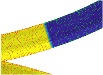
To obtain insight into the conditions for numerical convergence, we visually inspected the activity profiles by plotting  $j(\boldsymbol {x}_s)$. We found that numerical convergence is associated with having a sufficiently smooth interface between the active and inert sides of the particle. An illustrative example of this smoothness is provided in figure 2. The BEM code solves for the concentration at nodes of the particle mesh (coloured points). The red points represent catalytically active nodes of the mesh, while the green points represent inert nodes. The area elements of the mesh are coloured by interpolation from the surrounding nodes; blue represents inert and yellow represents active. The interface between the inert and active sides shows that the active and inert nodes are separated. Moreover, the interface between the two sides is smooth and approximately lies within a plane containing a circular cross-section of the article. The slight roughness observed is due to slight differences/non-uniformity between the local density of nodes (which are distributed during the meshing process on the two sides). For future work, we suggest that refinement of the mesh near the interface could lead to gains in computational efficiency (requiring fewer nodes and elements for the same level of accuracy).
Close-up of a meshed interface for a lengthwise Janus particle under conditions of numerical convergence. The red points represent catalytically active nodes of the mesh, while the green points represent inert nodes. The area elements of the mesh are coloured by interpolation from the surrounding nodes; blue represents inert and yellow represents active.

With regard to computational efficiency, we note that application of the Lorentz reciprocal theorem can save significant computational time in that, for a given helix geometry, the six auxiliary problems for the Stokes equation only need to be solved once. Solving these problems yields the resistance matrix and tractions that can be used for any distribution of surface slip. Therefore, one can examine different distributions of catalytic coverage, surface mobility parameters, etc. without having to perform additional hydrodynamic calculations.
Solution of the system in (2.10) yields the particle velocity, but not the flow field  $\boldsymbol {u}(\boldsymbol {x})$. When desired, the flow field can be obtained by subsequent additional numerical solution of (2.18), subject to the (now completely known) boundary condition (2.4). One can then obtain the velocity field using the boundary integral equation
 \begin{equation} u_k(\boldsymbol{x}_0) ={-} \int_{\mathcal{S}} [ \mathcal{G}_{ik}(\boldsymbol{x}_0, \boldsymbol{x}) q_i ] \, {\textrm{d}}S, \quad \boldsymbol{x}_0 \in \mathcal{V}. \end{equation}
3. Results
3.1. Hydrodynamic resistance tensor
As our starting point, we consider the hydrodynamic resistance tensor  ${\boldsymbol{\mathsf{R}}}$ of a helical filament, as it is a key quantity entering into (2.10). Each row
 $j$ of
 ${\boldsymbol{\mathsf{R}}}$ can be obtained by solving auxiliary problem
 $(j)$ for rigid body motion of the helix and, from the solution for
 $\boldsymbol {u}^{(j)}$, calculating the force and torque on the particle. We can solve each auxiliary problem numerically, using the BEM.
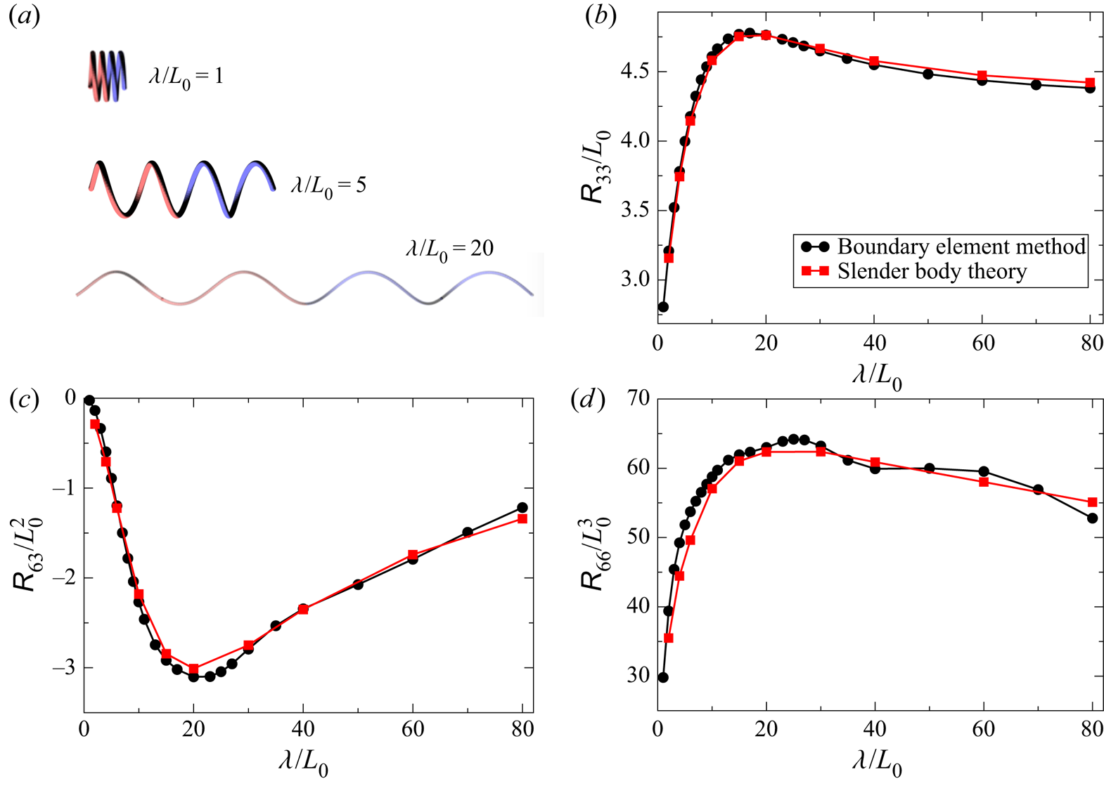
In figure 3, we consider an example problem in order to both validate our numerical scheme and to shed some light on how the hydrodynamic resistance of a helix depends on its shape. Specifically, we obtain the components of  ${\boldsymbol{\mathsf{R}}}$ as a function of pitch
 $\lambda$ for a helix with fixed contour length
 $\mathcal {L}$, fixed tube radius
 $r_0$, and fixed contour radius
 $R$. This variation of
 $\lambda$ can be regarded as ‘stretching out’ an initially tightly coiled helix, as shown schematically in figure 3(a). Of particular interest are
 ${\mathsf{R}}_{33}$,
 ${\mathsf{R}}_{36} = {\mathsf{R}}_{63}$ and
 ${\mathsf{R}}_{66}$. The quantity
 ${\mathsf{R}}_{33}$ represents the coefficient for hydrodynamic drag (in the
 $\hat {\boldsymbol {z}}$ direction) on a helix translating along its screw axis, i.e. in the
 $\hat {\boldsymbol {z}}$ direction. Likewise,
 ${\mathsf{R}}_{66}$ represents the rotational drag coefficient for rotation around the helix axis. Finally,
 ${\mathsf{R}}_{63}$ represents translational–rotational coupling, i.e. the torque in the
 $\hat {\boldsymbol {z}}$ direction that results when a helix translates in the
 $\hat {\boldsymbol {z}}$ direction, or the force in the
 $\hat {\boldsymbol {z}}$ direction that results when a helix rotates around the
 $\hat {\boldsymbol {z}}$ axis.
(a) Schematic illustration of three helices with different values of pitch  $\lambda$, but identical contour length
 $\mathcal {L}/L_0 = 57.5$, contour radius
 $R/L_0 = 2.5$ and filament radius
 $r_0/L_0 = 0.265$. (b) Variation of
 ${\mathsf{R}}_{33}$, the dimensionless drag coefficient for translational motion along the axis, with
 $\lambda$. Black circles were obtained with the boundary element method, and red circles were obtained by the SBT described in Koens & Lauga (Reference Koens and Lauga2014). (c) Variation of the translational–rotational coupling coefficient
 ${\mathsf{R}}_{63}$ with
 $\lambda$. Note that
 ${\mathsf{R}}_{63} = {\mathsf{R}}_{36}$. (d) Variation of
 ${\mathsf{R}}_{66}$, the dimensionless rotational drag coefficient for rotation around the helix axis, as a function of
 $\lambda$.

Interestingly, we obtain non-monotonic behaviour for all three quantities shown in figure 3, with a minimum in  ${\mathsf{R}}_{63}$ and maxima in
 ${\mathsf{R}}_{33}$ and
 ${\mathsf{R}}_{66}$ appearing around
 $\lambda / L_0 \approx 20$. In order to cross-check our results, we also performed calculations with SBT, as described in the work of Koens & Lauga (Reference Koens and Lauga2014). The BEM and SBT broadly agree, except that with the BEM we obtain a slight oscillation in
 ${\mathsf{R}}_{66}$ as a function of
 $\lambda$ (figure 3d). The minor discrepancies between SBT and BEM could be due to the fact the SBT does not account for the circumferential variation of hydrodynamic stress (i.e. variation with
 $\phi$) over the surface of the particle. Moreover, the SBT equations in Koens & Lauga (Reference Koens and Lauga2014) assume that the cross-sectional radius of the particle varies as
 $r_b \sqrt {1-s^{2}}$, where
 $r_b$ is the maximum thickness; recall that our particle has uniform cross-section, except for the hemispherical endcaps.
We have also sought to compare our results with resistive force theory (RFT), using the expressions in Palusa et al. (Reference Palusa, de Graaf, Brown and Morozov2018) and Chattopadhyay et al. (Reference Chattopadhyay, Moldovan, Yeung and Wu2006). For calculation of the components of the resistance tensor, RFT treats the filament as consisting of hydrodynamically non-interacting rod-like segments. We obtained semi-quantitative agreement of RFT with SBT and BEM for the variation of  ${\mathsf{R}}_{36}$ with
 $\lambda$, semi-quantitative agreement for the variation of
 ${\mathsf{R}}_{{66}}$ with
 $\lambda$ for
 $\lambda /L_0 > 30$, and poor agreement for
 ${\mathsf{R}}_{33}$. It has been known since the work of Rodenborn et al. that RFT generally has poor quantitative agreement with theories that include non-local hydrodynamic interactions, such as SBT and BEM; therefore, we do not include the RFT results here.
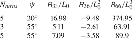
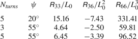
As another check, we consider the helix geometries studied experimentally by Purcell (Reference Purcell1997) using metal wire and numerically with the regularized BEM by Cortez et al. (Reference Cortez, Fauci and Medovikov2005). Specifically, both works consider a helix with fixed end-to-end distance  $L$, number of turns
 $L/\lambda$, pitch angle
 $\psi = 2 {\rm \pi}R / \lambda$ and filament radius
 $r_0$, with
 $R$ determined from the fixed parameters. The treatment of the two helix ends is not explicitly reported in Cortez et al. (Reference Cortez, Fauci and Medovikov2005). The quantities
 $A$,
 $B$ and
 $D$ in Purcell (Reference Purcell1997) correspond to our
 ${\mathsf{R}}_{33}$,
 ${\mathsf{R}}_{36}$ and
 ${\mathsf{R}}_{66}$, respectively, and are tabulated in table 2. Likewise, in Cortez et al. (Reference Cortez, Fauci and Medovikov2005), the quantities
 ${\mathsf{T}}_{33}$,
 ${\mathsf{P}}_{33}$ and
 ${\mathsf{R}}_{33}$, correspond to
 ${\mathsf{R}}_{33}$,
 ${\mathsf{R}}_{36}$ and
 ${\mathsf{R}}_{66}$ in this work, and are tabulated in table 3. However, the quantities given in Purcell (Reference Purcell1997) and Cortez et al. (Reference Cortez, Fauci and Medovikov2005) are dimensional. We rescaled the quantities to be dimensionless in table 2 and table 3 by choosing the length scale to be
 $L_0 = \frac {2}{5}R$. Moreover, for the coordinate system chosen in this work, the off diagonal
 ${\mathsf{R}}_{36}$ is negative for a right-handed helix, as also noted by Purcell (Purcell Reference Purcell1997). The sign can be understood from the force balance on a helix segment in RFT (Poon Reference Poon2013). In table 4, we show that our implementation of the BEM has good agreement with Cortez et al. (Reference Cortez, Fauci and Medovikov2005) and good convergence with mesh refinement. The slight discrepancy between our results and those of Cortez et al. (Reference Cortez, Fauci and Medovikov2005) may be due to the treatment of the helix ends.
Experimental measurements from Purcell (Reference Purcell1997), rescaled to be dimensionless for comparison with our BEM results in table 4.

Numerical calculations from Cortez et al. (Reference Cortez, Fauci and Medovikov2005), rescaled to be dimensionless for comparison with our BEM results in table 4.

Results of BEM numerical calculations for resistance matrix of a helix. Per cent error is calculated with respect to the numerical data of Cortez et al. (Reference Cortez, Fauci and Medovikov2005).

3.2. Lengthwise Janus chemically active particle
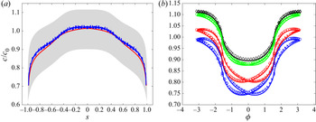
Now we consider the effect of catalytic activity for a lengthwise Janus particle, beginning with the concentration field  $c$. In order to validate our boundary element numerical method, we compare the results of BEM for
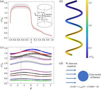
 $c$ against predictions of a slender body approach that will be developed in detail in § 3.5 below. In figure 4(a), the grey area shows the range of variation of concentration on the surface of a particle as a function of tangential position
 $s$, determined with the BEM. Note that for each tangential position
 $s$ there is a range of values of concentration
 $c$, indicated by the vertical extent of the grey area, due to variation of
 $c$ with the circumferential angle
 $\phi$. The red curve is the prediction of SBT, for this geometry and activity profile, of the circumferentially averaged concentration on the particle surface as a function of
 $s$. The red curve shows excellent agreement with the variation of the grey region with
 $s$. In figure 4(b), we show the concentration on the surface of the particle; the variation of
 $c$ is dominated by tangential gradients, but circumferential variation is also clearly visible.
(a) Concentration with respect to the tangential position  $s$ for
 $\lambda /L_0 = 5$ and other parameters the same as in figure. 3. The shaded grey area shows the range of values that were obtained for
 $c$ for a given
 $s$ and various circumferential angles
 $\phi$ (individual data points are omitted for clarity). The solid curve is a theoretical expression for the circumferentially averaged concentration obtained with SBT. The inset shows the definition of the angle
 $\phi$ with respect to the local
 $\hat {\boldsymbol {n}}_h$ at a position
 $s$ along the centreline, as well as decomposition of the surface concentration gradient
 $\nabla _s c$ into tangential and circumferential (i.e. in the plane of the helix cross-section at
 $s$) components. (b) Three-dimensional plot of the concentration
 $c$ on the surface of the particle. (c) Variation of concentration
 $c$ as a function of circumferential angle
 $\phi$ for various values of
 $s$. The dashed line indicates
 $\phi = -{\rm \pi} /2$. (d) Schematic illustration of the modification of the SBT to obtain the circumferential variation of concentration around the cross-section at
 $s$. To obtain the solid curves in (c), it is assumed that the local concentration gradient created by the rest of the particle induces a dipolar variation of concentration on the filament surface with respect to
 $\phi$. In (c), the values of
 $s$ are as follows: black circles,
 $s = -0.95$; blue circles,
 $s = -0.65$; red circles,
 $s = -0.15$; magenta diamonds,
 $s = -0.02$; blue diamonds,
 $s = 0$; magenta crosses,
 $s = 0.05$; black crosses,
 $s = 0.15$; red crosses,
 $s = 0.35$; blue crosses,
 $s = 0.65$; green crosses,
 $s = 0.85$.

In order to gain a better understanding of the circumferential variation, we plot  $c$ as function of
 $\phi$ for different values of
 $s$ in figure 4(c). The symbols were obtained with the BEM. For each value of
 $s$, we find that
 $c$ varies with
 $\phi$ in a sinusoidal fashion, with the amplitude and phase depending on
 $s$. Interestingly, in the inert region of the particle (
 $s > 0$), the curves generally have maxima that approach
 $\phi \approx -{\rm \pi} /2$ as
 $s$ approaches
 $s = 1$. As detailed in § 3.5, we extend SBT to account for circumferential variation of concentration. Briefly, we hypothesize that the concentration on the surface of a circular cross-section of the filament, at a given
 $s$, is polarized by an ambient gradient in concentration created by the rest of the particle. This hypothesis is shown schematically in figure 4(d). By making an analogy with a cylinder in uniform potential flow, we are able to obtain the solid curves in figure 4(c).
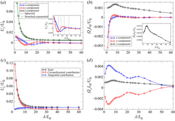
Now we consider the velocity of the lengthwise Janus particle as a function of pitch  $\lambda$, with other geometric parameters the same as in figure 3. In figure 5(a), we show the three components of translational velocity. As one might expect,
 $U_z$ is significantly greater in magnitude than
 $U_x$ and
 $U_y$. Moreover, is
 $U_z$ everywhere positive, as the particle is repelled from regions of high concentration. For
 $\lambda /L_0 \gg 1$,
 $U_z$ asymptotes to a constant value, since the filament geometry approaches the limit of a straight cylinder with hemispherical ends. For comparison, we plotted the velocity of a spheroidal particle with major axis diameter
 $\mathcal {L}$ and minor axis diameter
 $2r$ (dashed line), obtained from Ibrahim et al. (Reference Ibrahim, Golestanian and Liverpool2018). The asymptotic value and the velocity of the spheroid are comparable, as expected. As a side note, we find that the variation of
 $U_z$ with
 $\lambda$ is captured by a stretched exponential fit.
(a) Components of the translational velocity  $\boldsymbol {U}$ of a lengthwise Janus particle as a function of pitch
 $\lambda$ and parameters
 $r$,
 $\mathcal {L}$ and
 $R$ the same as in figure 3. In the main figure, the dashed line shows the value of
 $U_z$ for a spheroidal particle with major axis diameter
 $\mathcal {L}$ and minor axis diameter
 $2r$, as determined from Ibrahim, Golestanian & Liverpool (Reference Ibrahim, Golestanian and Liverpool2018). The green curve shows a stretched exponential fit to
 $U_z$. In the inset, the dashed lines indicate values of
 $\lambda$ for which the number of turns is a half-integer. (b) Components of the angular velocity
 $\boldsymbol {\varOmega }$ of a lengthwise Janus particle as a function of pitch
 $\lambda$ and other parameters the same as in figure 3. The inset shows the peak in
 $\varOmega _z$. (c) The contributions of circumferential and tangential concentration gradients to
 $U_z$ as a function of
 $\lambda$. (d) The contributions of circumferential and tangential concentration gradients to
 $\varOmega _z$ as a function of
 $\lambda$.

The components  $U_x$ and
 $U_y$ exhibit a decaying oscillatory behaviour as a function of
 $\lambda$. As expected from symmetry considerations,
 $U_x$ and
 $U_y$ approach zero for large
 $\lambda$. In the inset of figure 5(a), we show the oscillatory behaviour in closer detail. Hypothesizing that the oscillation is due to end effects for a finite length helix, we indicate with dashed lines the values of
 $\lambda$ for which the number of turns
 $N_{{turns}}$ is a half-integer. These values approximately correspond to the locations of the maxima and minima of
 $U_x$ and
 $U_y$, giving credence to our hypothesis.
Now we consider the decomposition of the surface concentration gradient into circumferential and tangential components. In figure 5(c) and 5(d), we observe that the contributions of circumferential concentration gradients to  $U_z$ and
 $\varOmega _z$ are surprisingly important. Concerning
 $U_z$, one expects that, for large pitch, i.e. for a geometry approaching that of a straight rod, tangential gradients should dominate circumferential gradients, and this is indeed the case in figure 5(c). However, we also find a cross-over at intermediate pitch, and circumferential gradients are dominant at low pitch. Moreover, tangential and circumferential gradients compete with regard to rotation around the helix screw axis: tangential gradients tend to rotate the particle counter-clockwise around this axis, while circumferential gradients drive clockwise rotation (figure 5d). As a result, the angular velocity
 $\varOmega _z$ is small. These findings suggest designing an activity profile to deliberately suppress one of the two contributions to particle motion.
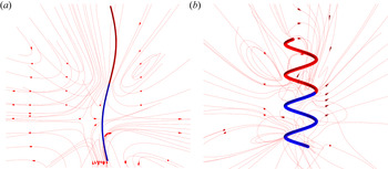
The significance of circumferential gradients for low pitch helices additionally has impact on the flow field in the vicinity of the particle. In figure 6, we show streamlines (obtained in a stationary frame) in the vicinity of helices with small and large pitch. For the large pitch helix, the flow field is only weakly perturbed from being axisymmetric. A stagnation point is identifiable near the middle of the active side of the particle. Noting that fluid is drawn into the poles of the particle and expelled from the sides, we expect that the particle is a hydrodynamic ‘puller’. For the small pitch helix, in contrast, the structure of streamlines is much more complex. Streamlines can wrap around the helix surface over and over, owing to the strong circumferential flows. However, a stagnation point and a puller-like structure of streamlines in the far field are still recognizable.
Streamlines (obtained in the stationary frame) of flow in the vicinity of a helix with (a) large pitch ( $\lambda /L_0 = 60$) and (b) small pitch (
 $\lambda /L_0 = 5$).

As an additional note, from the peak in  ${\mathsf{R}}_{33}$ in figure 3(b), one might expect a corresponding minimum in
 $U_z$ at the same value of
 $\lambda$. However, in figure 5(a), we observe monotonic decay of
 $U_z$ with
 $\lambda$. To resolve this apparent paradox, we note that in solving (2.10), we effectively multiply both sides of the equation by the inverse of the resistance matrix, i.e. the mobility matrix
 ${\boldsymbol{\mathsf{M}}} \equiv {\boldsymbol{\mathsf{R}}}^{-1}$. The extrema of the mobility matrix components may not appear at the same
 $\lambda$ as the extrema of the resistance matrix. Moreover, the components of the right-hand side vector
 $\boldsymbol {b}$ will also vary with
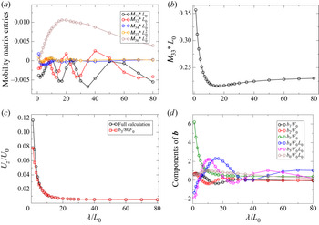
 $\lambda$. In figure 7(a,b), we show the entries of the third row of the mobility matrix. The diagonal entry
 ${\mathsf{M}}_{33}$ clearly dominates the third row, which determines
 $U_z$. Moreover,
 ${\mathsf{M}}_{33}$ is approximately flat over a broad range of
 $\lambda /L_0$, and exhibits only a very shallow minimum at
 $\lambda /L_0 \approx 13$. This finding permits the approximation shown in figure 7(c). Taking
 $6 {\rm \pi}/80 \approx 0.236$ as a characteristic value of the flat region of figure 7(b), we approximate
 $U_z/U_0$ as
 $b_3 / 80 F_0$, obtaining good agreement with the complete calculation. Thus, translation along the axis is largely determined by the
 $z$-component of the effective ‘force’
 $\boldsymbol {b}$, and coupling to other modes of motion is negligible. Moreover, the variation of
 $U_z$ with
 $\lambda$ is determined, for most
 $\lambda$, by the variation of
 $b_3$ with
 $\lambda$. In figure 7(d), we show the variation of the components of
 $\boldsymbol {b}$ as a function of
 $\lambda$ for the lengthwise Janus particle. It can be observed that the dependence of
 $b_3$ on
 $\lambda$ resembles the dependence of
 $U_z$ on
 $\lambda$.
(a) Off-diagonal entries of the third row of the mobility tensor  ${\boldsymbol{\mathsf{M}}}$ as a function of pitch
 $\lambda$, and other parameters as given in figure 3. (b) Mobility tensor component
 ${\mathsf{M}}_{33}$ as a function of pitch
 $\lambda$. Note the difference in scale from (a); the diagonal entry dominates the third row of
 ${\boldsymbol{\mathsf{M}}}$. (c) Translational velocity component along the helix axis
 $U_z$ for a lengthwise Janus activity profile as a function of pitch (all other parameters are the same as in figure 5). The full calculation that takes into account all components of
 ${\boldsymbol{\mathsf{M}}}$ and the right-hand side vector
 $\boldsymbol {b}$ shows good agreement with an approximate solution obtained as
 $b_3/80F_0$, where
 ${6 {\rm \pi}}/80$ is chosen as a characteristic value of the ‘flat’ part of the curve in (b). (d) Components of the right-hand side vector
 $\boldsymbol {b}$ as a function of pitch
 $\lambda$ for the lengthwise Janus particle.

3.3. The ‘$z$-wise’ Janus particle

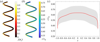
We now consider the ‘ $z$-wise’ Janus particle (figure 8a). For this particle, one can expect circumferential gradients to be strong, while tangential gradients should be weak by symmetry of the activity profile along the contour. These expectations are borne out by our numerical calculations of the concentration, shown in figure 8(b) and figure 8(c). In particular, we note that the broad width of the grey area in figure 8(c) for fixed
 $s$, at most values of
 $s$, which indicates strong circumferential gradients. Additionally, the circumferentially averaged concentration (red curve, obtained by SBT) is fairly flat, except for the helix ends, indicating that tangential gradients are small.
(a) Dimensionless catalytic activity  $j(\boldsymbol {x}_s)$ on the surface of a
 $z$-wise Janus particle with
 $\lambda /L_0 = 5$ and parameters
 $r$,
 $\mathcal {L}$ and
 $R$ the same as in figure 3. (b) Three-dimensional plot of the concentration
 $c$ on the surface of the particle. (c) Concentration with respect to the tangential position
 $s$. The shaded grey area shows the range of values that were obtained for
 $c$ for a given
 $s$ and various circumferential angles
 $\phi$ (not shown). The solid curve is a theoretical expression for the circumferentially averaged concentration obtained with SBT.

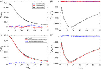
Turning to the results for the velocity, we find that the particle has strong rotation around the screw axis, i.e. the  $z$-axis, while rotation around the perpendicular axes is negligible (figure 9b). This is useful for applications – the particle will show strong directed motion along the screw axis direction, and will not tumble haphazardly. Concerning the decomposition into tangential and circumferential contributions, we find that our expectations are confirmed (figure 9c,d).
(a) Components of the translational velocity  $\boldsymbol {U}$ of a
 $z$-wise Janus particle as a function of pitch
 $\lambda$, with parameters
 $r$,
 $\mathcal {L}$ and
 $R$ the same as in figure 3. (b) Components of the angular velocity
 $\boldsymbol {\varOmega }$. (c) The
 $z$-component
 $U_z$ of the particle translational velocity as a function of pitch, as well as the contributions of circumferential and tangential concentration gradients to
 $U_z$. (d) The
 $z$-component
 $\varOmega _z$ of the particle angular velocity as a function of pitch, as well as the contributions of circumferential and tangential concentration gradients.

3.4. ‘Inside–outside’ Janus particle
Finally, we consider the ‘inside–outside’ Janus particle. As one might expect, the circumferential variations in the concentration field  $c$ are substantial (see figure 10a), and dominate the tangential variations. Following the slender body approach in (3.5), we can identify three distinct factors that contribute to the concentration profile. First, the averaged SBT (red line) again lies very well within the variation of the concentration field (grey area). It also matches the mean concentration field (blue line) to a high degree, despite only accounting for the averaged catalytic activity (see § 3.5.2). As expected, it is symmetric with respect to
 $s$. However, for this activity profile, two additional factors lead to circumferential variation (for a given
 $s$) of the concentration profile (see figure 10b).
(a) Concentration with respect to the tangential position  $s$ for an ‘inside–outside’ Janus helix. The shaded grey area shows the range of values that were obtained for
 $c$ for a given
 $s$ and various circumferential angles
 $\phi$ (not shown), and the blue line shows the mean value as a function of
 $s$. The solid curve is a theoretical expression for the circumferentially averaged concentration obtained with SBT. (b) Variation of concentration
 $c$ as a function of circumferential angle
 $\phi$ for various values of
 $s$. The values of
 $s$ are as follows: blue circles,
 $s = -0.85$; blue crosses,
 $s = 0.85$; red circles,
 $s = -0.65$; red crosses,
 $s = 0.65$; green circles,
 $s = -0.35$; green crosses,
 $s = 0.35$; black diamonds,
 $s = 0$.

The second factor is the circumferential variation of the activity profile, i.e. the dependence of  $j(\boldsymbol {x}_s)$ on
 $\phi$. In the slender body approach, this factor can be accounted for in the construction of the inner solution. Specifically, we solve for the concentration field around an infinite, half-covered cylinder with translational symmetry via a series expansion. Therefore, this factor can be reduced to and solved in two dimensions. The third factor is, as before, polarization of the surface concentration at
 $s$ induced by the ambient concentration gradient created by the rest of the particle. Concerning these second and third factors, the contribution from the local catalytic activity (i.e. the second factor) is dominant, and ensures that the minimal concentration is always close to the centre of the inert region (
 $\phi \approx 0$) and the maximum on the opposite side (
 $\phi \approx \pm {\rm \pi}$). Away from the centre (
 $s = 0$) of the helix (represented by black diamonds in figure 10b), the average concentration drops, and a circumferential asymmetry develops. This circumferential asymmetry is due to the third factor, i.e. the dipolar polarization introduced by the rest of the particle. Due to the symmetry of the activity profile along the contour, the disturbances at locations
 $s$ and
 $-s$ are mirror symmetric with respect to
 $s = 0$. The asymmetry becomes more significant further away from the centre.
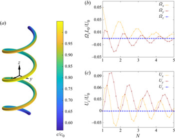
Analysing the velocity components for ‘inside–outside’ Janus helices (see figure 11) we immediately see that, due to their symmetric design, both the  $U_z$ and
 $\varOmega _z$ components vanish. All other components exhibit a decaying oscillation with respect to the total number of turns
 $N$ in the helix. These particles have completely different trajectories compared with the first two examples and are not propelled in the direction of the screw axis. For both the translation and the rotational velocity, the minima and maxima in the
 $x$-component lead the corresponding maxima and minima in the
 $y$-component by a quarter turn. This can again be understood by our hypothesis that the movement in
 $xy$ plane is mainly due to end effects. In order to illustrate this, we will take a closer look at the
 $U_y$ component. Recall that our helices are constructed by fixing the bottom end to point in the
 $y$ direction; the tangential direction of top end depends on the number of turns
 $N$ and other parameters. For an integer number of turns, the ends point in opposite (
 $y$ and
 $-y$) directions and balance each other. Upon increasing
 $N$, the top (
 $s = 1$) rotates by an angle
 $\gamma =2 {\rm \pi}\mod (N,1)$ and increases its
 $y$- component
 $\hat {\boldsymbol {t}}_h (s = 1) \boldsymbol {\cdot } \hat {y} \propto -\cos (\gamma )$, while the bottom end stays in place. At the next half-integer turn, the top and the bottom end are pointing in the same direction, i.e.
 $y$, and the overall velocity
 $U_y$ reaches a maximum. Further growth of the helix causes the top contribution to shrink, until the two balance each other again at the next full turn. Note that
 $U_y$ is never negative because of the construction of the helix. For the other three non-zero velocities,
 $U_x$,
 $\varOmega _x$ and
 $\varOmega _y$, the periodicity can be explained similarly. When inspecting
 $U_x$ more closely, we see that these end effects do not entirely account for the variation of the velocity, e.g.
 $U_x$ is not exactly
 $0$ at
 $N=1,2,3,4,5$. This offset is caused by the finite size of the body and can be understood best by examining the details of the
 $N = 1$ helix. The centre of this helix (
 $s = 0$) lies on the
 $x$-axis, and circumferential variations in the concentration field at
 $s = 0$ can only induce movement in the
 $x$-direction. For any off-centre values
 $s_0 \neq 0$, the helix can have
 $y$-contributions. However, due to the symmetry in the concentration field, the
 $y$-contribution at
 $s=-s_0$ has to be of equal magnitude and opposite sign. Thus, the two cancel each other out, and there is no movement in the
 $y$- direction for helices with an integer number of turns. This is not true for the
 $x$-component. The
 $s = 0$ contribution to
 $U_x$ is counteracted by the points
 $\pm s_0=\pm {1}/{4N}$ half a turn up and down the helix axis, which have normal vectors
 $\hat {\boldsymbol {n}}_h(s_0) = \hat {\boldsymbol {n}}_h(-s_0)$ in the opposite direction, i.e.
 $\hat {\boldsymbol {n}}_h(s_0) = -\hat {\boldsymbol {n}}_h(0)$. However, the finite size of the helix causes the concentration field to decrease away from the helix centre towards the ends. The two contributions at
 $\pm s_0$ do not add up to the same magnitude as at the centre, and the particle has a net velocity in the
 $x$-direction. In summary, we consider that a finite size effect is responsible for the slight shift of the zeros of
 $U_x$, as a function of
 $N$, away from integer values of
 $N$ (figure 11c).
(a) Three-dimensional plot of the concentration  $c$ on the surface of the ‘inside–outside’ Janus helix. (b) Components of the transitional velocity
 $\boldsymbol {U}$ as a function of the number of turns
 $N$ and pitch
 $\lambda /L_0 = 5$, contour radius
 $R/L_0=2.5$ and filament radius
 $r_0/L_0 = 0.265$. (c) Components of the and angular velocity
 $\boldsymbol {\varOmega }$ as a function of the number of turns
 $N$.

3.5. SBT for helix surface concentration
In this section, we introduce an analytical approximation that relies on the ‘slenderness’ parameter  $\epsilon \equiv 2r_0 / \mathscr {L}$ being very small, i.e.
 $\epsilon \ll 1$. We neglect the role of the hemispherical caps. Our treatment is influenced by the work in Ibrahim et al. (Reference Ibrahim, Golestanian and Liverpool2018) and Schnitzer & Yariv (Reference Schnitzer and Yariv2015) on slender, axisymmetric self-phoretic particles, as well as Keller & Rubinow (Reference Keller and Rubinow1976) on the hydrodynamic resistance of slender bodies. In particular, our presentation in § 3.5.1 closely follows the formal manipulations and asymptotic mathematics of Keller & Rubinow (Reference Keller and Rubinow1976). It can be regarded as transposing some of their results to the context of Laplace's equation and active colloids. Our presentation in the subsequent section, in contrast, is intended as a phenomenological, physically motivated attempt to model circumferential variations of concentration. It is developed on the basis of a physical hypothesis and a physical analogy to potential flow. Specifically, the connection with potential flow is possible because the concentration field in steady-state diffusion and the velocity potential in potential flow are both governed by Laplace's equation.
We note that, recently, a systematic and rigorous derivation of SBT for a chemically active filament was published by Katsamba, Michelin & Montenegro-Johnson (Reference Katsamba, Michelin and Montenegro-Johnson2020), who work from the alternative basis provided by Koens & Lauga (Reference Koens and Lauga2018). One advantage of working from that basis is that it facilitates consideration of circumferential variation of the surface stress. Thus, Katsamba et al. (Reference Katsamba, Michelin and Montenegro-Johnson2020) are able to (numerically) calculate particle velocities in the framework of SBT; in that sense, their formulation of SBT is complete. Here, we restrict our attention to calculation of the concentration field. Additionally, we make no pretence to the level of formal rigor and systematic mathematical development provided in Katsamba et al. (Reference Katsamba, Michelin and Montenegro-Johnson2020). However, our brief treatment may provide an accessible point of entry into SBT for some readers. Additionally, by being grounded in a physical model, it sheds light on underlying physical mechanisms.
For the slender body analysis, the governing equations for the concentration will be non-dimensionalized using a characteristic length  $L_0 \equiv \mathscr {L}/2$ (i.e. the half-length of the particle) and characteristic concentration
 $C_0 \equiv \kappa r_0/ D$, distinct from the previously defined
 $c_0$. Accordingly, the equations become
 \begin{equation} \nabla^{2} c = 0, \end{equation}
and
 \begin{equation} \hat{\boldsymbol{n}} \boldsymbol{\cdot} \boldsymbol{\nabla} c ={-}j(s)/\epsilon, \end{equation}
with  $c(|\boldsymbol {x}| \rightarrow \infty ) = 0$, where
 $c$ and the gradient operator are understood to be dimensionless. We will use this non-dimensionalization for the rest of § 3.5.
3.5.1. Circumferentially averaged concentration
Using asymptotic expansions, the solution for  $c(\boldsymbol {x})$ can be separated into ‘inner’ and ‘outer’ regions in the limit
 $\epsilon \rightarrow 0$. The outer region is defined such that, for a position
 $\boldsymbol {x}$ in the outer region, the distance
 $r$ to the closest point on the helix backbone is
 ${O}(1)$, i.e. much larger than
 $\epsilon$ in the limit
 $\epsilon \rightarrow 0$. In this region, we can represent the concentration as being due to a distribution of sources
 $\alpha (s)$ along an infinitesimally thin space curve
 \begin{equation} c_{{out}}(\boldsymbol{x}) = \int_{{-}1}^{1} \frac{\alpha(s')}{|\boldsymbol{x} - \boldsymbol{x}_h(s')|} \, {\textrm{d}}s' . \end{equation}
In the inner region, where  $r$ is
 ${O}(\epsilon )$ as
 $\epsilon \rightarrow 0$, the particle resembles an infinitely long cylinder. Here, we introduce the stretched coordinate
 $\rho \equiv r/\epsilon$. Following the logic of Schnitzer & Yariv (Reference Schnitzer and Yariv2015), we integrate (3.1) (assuming an effectively two-dimensional problem) and impose the boundary condition in (3.2) to obtain
 \begin{equation} c_{{in}}(\rho, s) = C(s; \epsilon) - j(s) \ln \rho, \end{equation}
where the function  $C(s;\epsilon )$ will be determined by matching to the outer solution. Physically, the logarithmic term can be interpreted as the (two-dimensional) concentration field due to an infinitely long and uniformly active cylinder. The function
 $C(s;\epsilon )$ is an ‘integration constant’ for the contour position
 $s$.
Our next task is to perform asymptotic matching between the inner region and outer region in the limit  $\epsilon \rightarrow 0$ to obtain
 $C(s;\epsilon )$ and
 $\alpha (s)$. Concerning the outer solution, we consider a position
 $\boldsymbol {x} = \boldsymbol {x}_h(s) + \boldsymbol {r}$, with
 $\boldsymbol {r} \boldsymbol {\cdot } \hat {\boldsymbol {t}}(s) = 0$ (i.e. the position
 $\boldsymbol {x}$ is in the plane defined by the particle cross-section at
 $s$) and
 $|\boldsymbol {r}| =r$. We wish to examine the limits
 $\boldsymbol {r} \rightarrow 0$ as
 $\epsilon \rightarrow 0$. We expect that the concentration
 $c_{{out}}(\boldsymbol {r},s) \equiv c_{{out}}(\boldsymbol {x}_h(s) + \boldsymbol {r})$ is singular as
 $\boldsymbol {r} \rightarrow 0$, since the domain of the integral includes
 $s$ itself, and since the evaluation point
 $\boldsymbol {x}$ approaches the helix backbone as
 $\boldsymbol {r} \rightarrow 0$.
In the following, we closely follow the procedure in appendix A of Keller & Rubinow (Reference Keller and Rubinow1976). Our aim is to isolate the singularity, i.e. move it out of the integral, and evaluate it analytically. First, we first change the integration variable  $q=s'-s$ in (3.3)
 \begin{equation} c_{{out}}(\boldsymbol{x}) = \int_{-(1+s)}^{1+s} \frac{\alpha(s+q)}{|\boldsymbol{x}_h(s) + \boldsymbol{r} - \boldsymbol{x}_h(s+q)|} \, {\textrm{d}}q. \end{equation}
We define  $\boldsymbol {R}_0 \equiv \boldsymbol {x}_h(s) - \boldsymbol {x}_h(s + q)$, with
 $R_0 \equiv |\boldsymbol {R}_0|$, as well as
 \begin{equation} R^{2} \equiv |\boldsymbol{R}_0 + \boldsymbol{r}|^{2} = R_0^{2} + 2 \boldsymbol{r} \boldsymbol{\cdot} \boldsymbol{R}_0 + r^{2}. \end{equation}
We also define the quantity  $K^{2}(\boldsymbol {R}_0, \boldsymbol {r})$ by
 $R^{2} \equiv r^{2} + K^{2} q^{2}$. The usefulness of
 $K$ will become apparent shortly, when discussing the limit
 $q \rightarrow 0$. The integral can be rewritten as
 \begin{equation} c_{{out}}(\boldsymbol{x}) = \int_{-(1+s)}^{1+s} \frac{\alpha(s+q)}{R} \, {\textrm{d}}q = \int_{-(1+s)}^{1+s} \frac{\alpha(s+q)}{\sqrt{r^{2} + K^{2} q^{2}}} \, {\textrm{d}}q. \end{equation}
For small  $q$, we can expand
 $\boldsymbol {R}_0$ in powers of
 $q$, and thereby obtain the following:
 \begin{equation} {{R}_0^{2} + 2 \boldsymbol{r} \boldsymbol{\cdot} \boldsymbol{R}_0} = \left(\frac{\partial \boldsymbol{x}_h}{\partial s}\right)^{2} q^{2} - \left(\frac{\partial^{2} \boldsymbol{x}_h}{\partial s^{2}} \boldsymbol{\cdot} \boldsymbol{r} \right) q^{2} + {O}(q^{3}). \end{equation}
The vector  $\boldsymbol {i} \equiv {\partial \boldsymbol {x}_h}/{\partial s}$ is tangent to the backbone and, since length is non-dimensionalized by
 $\mathscr {L}/2$ in this section, has unit length. We also define
 $\boldsymbol {i}_s \equiv {\partial ^{2} \boldsymbol {x}_h}/{\partial s^{2}}$, giving
 \begin{equation} {{R}_0^{2} + 2 \boldsymbol{r} \boldsymbol{\cdot} \boldsymbol{R}_0} = (1 - \boldsymbol{r} \boldsymbol{\cdot} \boldsymbol{i}_s ) q^{2} + {O}(q^{3}), \end{equation}
and
 \begin{equation} K^{2} = 1 - \boldsymbol{r} \boldsymbol{\cdot} \boldsymbol{i}_s + {O}(q). \end{equation}
From (3.7) and (3.10), it is apparent that, for small  $r$ and
 $q$, the singularity in the integral has the form
 $1/\sqrt {r^{2} + q^{2}}$. We attempt to isolate it from the integral as follows:
 \begin{equation} c_{{out}}(\boldsymbol{x}) = \int_{-(1+s)}^{1+s} \left[ \frac{\alpha(s+q)}{\sqrt{r^{2} + K^{2} q^{2}}} - \frac{\alpha(s)}{\sqrt{r^{2} + q^{2}}} \right] \, {\textrm{d}}q + \int_{-(1+s)}^{1+s} \frac{\alpha(s)}{\sqrt{r^{2} + q^{2}}} \, {\textrm{d}}q. \end{equation}
For  $r = 0$, the first integral is finite. This can be shown through a Laurent expansion of the first summand in powers of
 $q$; the singular term in the expansion,
 $\alpha (s)/q$, is exactly cancelled by the second summand. Interestingly, the numerator of the second integral has no dependence on
 $q$. Thus, the second integral can be evaluated analytically
 \begin{equation} \int_{0}^{t} \frac{{\textrm{d}}q}{\sqrt{r^{2} + q^{2}}} = [ \ln(\sqrt{t^{2} + r^{2}} + t) - \ln r ]. \end{equation}
We thus obtain
 \begin{align} \lim_{r \rightarrow 0} c_{{out}}(\boldsymbol{r},s) &= 2 \alpha (s) \ln \left(\frac{1}{r} \right) + \int_{-(1+s)}^{1-s} \left[ \frac{{\alpha}(s+q)}{|\boldsymbol{x}_h(s+ q) -\boldsymbol{x}_h(s)|} - \frac{ {\alpha}(s)}{|q|} \right] \, {\textrm{d}}q \nonumber\\ &\quad + \alpha(s) \ln [4 (1+s)(1-s)], \end{align}
or equivalently
 \begin{align} {\lim_{r \rightarrow 0}} c_{{out}}(\boldsymbol{r},s) &= 2 \alpha (s) \ln \left(\frac{2}{r} \right) + \int_{-(1+s)}^{1-s} \left[ \frac{{\alpha}(s+q)}{|\boldsymbol{x}_h(s+ q) -\boldsymbol{x}_h(s)|} - \frac{ {\alpha}(s)}{|q|} \right] \, {\textrm{d}}q \nonumber\\ &\quad + \alpha(s) \ln [(1+s)(1-s)], \end{align}
which exposes the logarithmic singularity. Note that (3.14) does not capture circumferential variations of concentration. Secondly, note that the ‘non-local’ integral contains information about the helical shape of the backbone. In asymptotic matching, we determine the unknown  $\alpha (s)$ and
 $C(s;\epsilon )$ from
 \begin{equation} \lim_{r \rightarrow 0} c_{{out}}(\boldsymbol{r},s) = \lim_{\rho \rightarrow \infty} c_{{in}}(\rho, s), \end{equation}
as  $\epsilon \rightarrow 0$. Matching (3.4) and (3.14), we find
 \begin{gather} \alpha(s) = \frac{1}{2} j(s), \end{gather}
 \begin{gather}C(s;\epsilon) = j(s) \ln \left(\frac{2}{\epsilon}\right) + C_{{o}}(s), \end{gather}
and
 \begin{equation} C_{{o}}(s) \equiv \frac{1}{2} \int_{-(1+s)}^{1-s} \left[ \frac{j(s+q)}{|\boldsymbol{x}_h(s+ q) -\boldsymbol{x}_h(s)|} - \frac{ j(s)}{|q|} \right] \, {\textrm{d}}q + \frac{1}{2} j(s) \ln [(1+s)(1-s)]. \end{equation}
Using (3.4) and associated expressions evaluated at the helix surface  $r = \epsilon$ (recall the non-dimensionalization of length in this section), we plot the red curve in figure 4(a) (reverting to the previous characteristic concentration
 $c_0$ in the figure). This curve runs through the scattered data points very well; however, it cannot account for the scatter, because (3.18) has no
 $\phi$ dependence. (Recall that the scatter represents the range of the variation of concentration in the angle
 $\phi$ for a given value of
 $s$.)
3.5.2. Circumferential variation of concentration
The slender body analysis in § 3.5.1 gave an expression for concentration that had no dependence on  $\phi$, and which can therefore be regarded as a circumferentially averaged concentration. This expression is useful for considering variations of concentration with
 $s$, i.e. the component of the surface gradient in the
 $\hat {\boldsymbol {t}}$ direction. However, the circumferential component of the surface concentration gradient could also contribute to self-propulsion, as discussed above.
Moreover, the numerical results clearly show a circumferential variation of concentration. In figure 4(c), we show the concentration on the surface of the lengthwise Janus particle, obtained via the BEM, as a function of  $\phi$ for various values of
 $s$. (Specifically, for each
 $s$, we consider values of
 $c$ on the surface for numerical mesh points within a small neighbourhood of
 $s$.) By inspection, there seems to be a sinusoidal dependence on
 $\phi$, with the phase depending on
 $s$. For
 $s$ within the active region, i.e.
 $s < 0$, the maximum in concentration is around
 $\phi = 0$ and the minimum at
 $\phi = \pm {\rm \pi}$, indicating that the circumferential variation in concentration is largely variation between the ‘inside’ and ‘outside’ of the helix. For the inert region
 $s > 0$, the maximum is shifted to approximately
 $-90^{\circ }$. This indicates that the circumferential variation of concentration is dominated by
 $\hat {\boldsymbol {b}}_h$. Note that
 $\hat {\boldsymbol {b}}_h$ has a
 $\hat {z}$ component and
 $\hat {\boldsymbol {n}}_h$ does not; since the maximum is at
 $-90^{\circ }$, the high concentration region is oriented towards the active side of the particle, i.e. towards
 $-\hat {z}$.
Based on these observations, we make the following hypothesis: at a point  $s$, the circumferential variation of concentration is due to polarization by the ‘external’ concentration gradient
 $\boldsymbol {\nabla } c$, i.e. the concentration gradient created by catalytic activity on other points of the helix. For instance, this would explain why, in the inert region of the helix, the high concentration region is oriented towards the active side of the helix. We can make an analogy with the classical problem of an infinite cylinder in uniform, two-dimensional potential flow, shown schematically in figure 4(d). This problem is also governed by Laplace's equation, subject to a no-flux boundary condition on the cylinder and a uniform gradient far from the cylinder. The solution can be obtained by linear superposition of the external gradient and a source dipole oriented in the opposite direction as the gradient. On the basis of this analogy, we expect that the amplitude of the sinusoidal variation at
 $s$ to be twice the magnitude of the component of external gradient in the plane defined by
 $\hat {\boldsymbol {n}}_h$ and
 $\hat {\boldsymbol {b}}_h$, i.e.
 $(\boldsymbol {1} - \hat {\boldsymbol {t}} _h \hat {\boldsymbol {t}}_h ) \boldsymbol {\cdot } \boldsymbol {\nabla } c$, evaluated at the centreline position
 $\boldsymbol {x}_{h}(s)$. Secondly, the phase of sinusoidal variation will be such that, for a particular
 $s$, the vector between the concentration minimum and concentration maximum (defined in three-dimensional space) will be aligned with the in-plane component of
 $\boldsymbol {\nabla } c$. Our analogy receives further motivation when we consider that we had regarded the tube surface as a ‘quasi-infinite cylinder’ when solving for the inner concentration in the previous section.
Based on these ideas, we proceed to consideration of  $\boldsymbol {\nabla } c$ for a lengthwise Janus helix. For a point
 $s > 0$ in the inert region, we can simply write
 \begin{equation} \boldsymbol{\nabla} c(\boldsymbol{x}_h) ={-}\frac{1}{2} \int_{{-}1}^{1} \frac{j(s') [\boldsymbol{x}_{h}(s) - \boldsymbol{x}_{h}(s')] \, {\textrm{d}}s'}{|\boldsymbol{x}_{h}(s) - \boldsymbol{x}_{h}(s') |^{3}}, \end{equation}
or
 \begin{equation} \boldsymbol{\nabla} c(\boldsymbol{x}_h) ={-}\frac{1}{2} \int_{{-}1}^{0} \frac{ [\boldsymbol{x}_{h}(s) - \boldsymbol{x}_{h}(s')] \, {\textrm{d}}s'}{|\boldsymbol{x}_{h}(s) - \boldsymbol{x}_{h}(s') |^{3}}. \end{equation}
For the second expression, we do not have any issues with integrating through a singularity, as  $s > 0$ in inert region. Specifically, we are interested in the normal and binormal components, since we need to know the orientation of the external gradient with respect to the local value of
 $\hat {\boldsymbol{n}}_h$. We obtain
 \begin{gather} \boldsymbol{\nabla} c(\boldsymbol{x}_h) \boldsymbol{\cdot} \hat{\boldsymbol{n}}_h ={-}\frac{1}{2} \int_{{-}1}^{0} \frac{ (\boldsymbol{x}_{h}(s) - \boldsymbol{x}_{h}(s')) \boldsymbol{\cdot} \hat{\boldsymbol{n}}_h(s) \, {\textrm{d}}s'}{|\boldsymbol{x}_{h}(s) - \boldsymbol{x}_{h}(s') |^{3} }, \end{gather}
 \begin{gather}\boldsymbol{\nabla} c(\boldsymbol{x}_h) \boldsymbol{\cdot} \hat{\boldsymbol{b}}_h ={-}\frac{1}{2} \int_{{-}1}^{0} \frac{ (\boldsymbol{x}_{h}(s) - \boldsymbol{x}_{h}(s')) \boldsymbol{\cdot} \hat{\boldsymbol{b}}_h(s) \, {\textrm{d}}s'}{|\boldsymbol{x}_{h}(s) - \boldsymbol{x}_{h}(s') |^{3} }. \end{gather}
We find the amplitude  $A$ of the sinusoidal variation as
 \begin{equation} A = 2 |\boldsymbol{\nabla} c(\boldsymbol{x}_h) \boldsymbol{\cdot} \hat{\boldsymbol{b}}_h + \boldsymbol{\nabla} c(\boldsymbol{x}_h) \boldsymbol{\cdot} \hat{\boldsymbol{n}}_h|, \end{equation}
and the phase  $\psi$ as
 \begin{equation} \psi = \textrm{arg}(\boldsymbol{\nabla} c(\boldsymbol{x}_h) \boldsymbol{\cdot} \hat{\boldsymbol{n}}_h + i \boldsymbol{\nabla} c(\boldsymbol{x}_h) \boldsymbol{\cdot} \hat{\boldsymbol{b}}_h( s) ). \end{equation}
Numerically integrating equations (3.21) and (3.22), we obtain the theoretical curves (solid lines) for the inert region of the particle (corresponding to the cross symbols) in figure 4(c).
For the active region of the particle  $(s < 0)$, the line integral in (3.19) has to been handled with care, since there is a singularity at
 $s = s'$. As in § 3.5.1, we follow the procedure in appendix A of Keller & Rubinow (Reference Keller and Rubinow1976) (see equations (A1) and (2) of that work). Via similar manipulations, we can isolate the singularities, obtaining
 \begin{align} &\boldsymbol{\nabla} c(\boldsymbol{x}_h(s)) \boldsymbol{\cdot} \hat{\boldsymbol{n}}_h ={-}\frac{1}{2} \left[ (\hat{\boldsymbol{n}}_h \boldsymbol{\cdot} \boldsymbol{i}_s) {\ln} \epsilon - \frac{1}{2} (\hat{\boldsymbol{n}}_h \boldsymbol{\cdot} \boldsymbol{i}_s) {\ln} [(1-s)(1+s)] \right. \nonumber\\ &\quad + \left.\hat{\boldsymbol{n}}_h(s) \boldsymbol{\cdot} \left( \int_{-(1+s)}^{1-s} \left[ \frac{\boldsymbol{R}}{R^{3}} - \frac{-\boldsymbol{i}(s) q + \left[- \frac{1}{2} \boldsymbol{i}_{s}(s) - j_s(s) \boldsymbol{i}(s) \right] q^{2}}{q^{3}} \right] \, {\textrm{d}}q \right) \right], \end{align}
and
 \begin{align} \boldsymbol{\nabla} c(\boldsymbol{x}_h(s)) \boldsymbol{\cdot} \hat{\boldsymbol{b}}_h ={-}\frac{1}{2} \hat{\boldsymbol{b}}_h(s) \boldsymbol{\cdot} \left( \int_{-(1+s)}^{1-s} \left[ \frac{\boldsymbol{R}}{R^{3}} - \frac{-\boldsymbol{i}(s) q + \left[- \frac{1}{2} \boldsymbol{i}_{s}(s) - j_s(s) \boldsymbol{i}(s) \right] q^{2}}{q^{3}} \right] \, {\textrm{d}}q \right), \end{align}
on the surface of the particle. Here,  $\boldsymbol {R} \equiv \boldsymbol {x}_h(s) - \boldsymbol {x}_h(s + q)$; quantities with
 $s$ subscripts indicate partial differentiation with respect to
 $s$; and the quantity
 $\boldsymbol {i} \equiv {\partial \boldsymbol {x}_h}/{\partial s}$, i.e.
 $\boldsymbol {i}$ is tangent to the contour and
 $\boldsymbol {i}_s$ is normal to it. The integrals can be evaluated numerically.
These expressions are valid over the whole contour of the particle, and in the inert region return the same results as (3.21) and (3.22). In figure 4(c), we plot the theoretical curves in the active region (circle symbols and diamond symbols). We obtain generally good agreement with the numerical data. Note that some of the disagreement is because the slender body expressions for the mean/circumferentially averaged concentration tend to underestimate  $c$ (possibly because these expressions neglect the catalytic endcap); if the theoretical curves were shifted upward, better agreement would be obtained. The greatest disagreement is for
 $s$ close to
 $s = 0$, i.e. the interface between the active and inert halves of the particle, but the theoretical curves still capture the general shape here.
3.5.3. Including circumferential variation of the activity profile
For a particle that has an activity profile that depends on  $\phi$, like the ‘inside–outside’ Janus particle, the initial approach to obtain the circumferentially averaged concentration does not change significantly. Using the circumferentially averaged activity profile
 $\bar j(s) \equiv ({1}/{2{\rm \pi} })\int _0^{2{\rm \pi} }j(s,\phi ) \, {\textrm {d}} \phi$ instead of
 $j(s)$ in the framework of § 3.5.1 is sufficient.
However, to obtain the circumferential variation of the concentration, additional terms in the inner solution are needed. In particular, for the ‘inside–outside’ Janus particle the azimuthal deviation from the average needs to be accounted for. One can achieve this by solving Laplace's equation in two dimensions for the boundary condition
 \begin{equation} \hat{\boldsymbol{n}} \boldsymbol{\cdot} \boldsymbol{\nabla} c (\boldsymbol{x})\vert_{r=r_0} = \left.\frac{\partial c}{\partial r} \right\vert_{r=r_0} ={-}\left.\left(\varTheta(\phi+{\rm \pi}/2)\varTheta(-\phi-{\rm \pi}/2){-\frac{1}{2}}\right)\right/\epsilon. \end{equation}
Essentially, one must solve for the concentration around a Janus cylinder with translational symmetry in the  $z$ direction. The parameters
 $a_n$ and
 $b_n$ in the multipole solution to Laplace's equation in two dimensions,
 \begin{equation} c(r,\theta)=a_0 \ln \left(\frac{1}{r}\right)+\sum_{n=1}^{\infty} \frac{a_n\cos(n\theta)+b_n\sin(n\theta)}{r^{n}}, \end{equation}
can be determined by applying the boundary conditions. One can substitute (3.28) into 3.27, substitute the step function  $\varTheta (\phi )$ by its Fourier series
 $\sum _{n} \beta _n \sin (n\phi )$ with
 $\beta _{n} \equiv ({-1}/{n{\rm \pi} })(\cos (n{\rm \pi} )-1)$, and match terms to determine
 $a_n$ and
 $b_n$.
4. Conclusions
Overall, the framework developed here provides a set of analytical and numerical tools for modelling self-phoretic helical particles. In particular, we outline methods to solve the two principal subproblems: diffusion of the product chemical and hydrodynamic reaction to the resulting slip velocity.
By including three-dimensional finite size effects, our extended SBT captures both tangential and circumferential variations in the concentration field surrounding the particle. We find that both the magnitude  $|c_{max}-c_{min}|$ and the phase
 $\phi _{max/min}$ of these (quasi-sinusoidal) variations depend on the geometric and chemical parameters of the helix (see §§ 3.2 and 3.4). In both cases, our analytical results are in line with numerical calculations done with the BEM. The BEM results for the second subproblem also show good agreement with previously published numerical and experimental data (§ 3.1). Although our development of SBT is limited to the chemical concentration field, the spatial variation of concentration near a catalytically active particle is of broad interest in active colloids, e.g. for understanding the phoretic motion of tracer particles (Aubret et al. Reference Aubret, Youssef, Sacanna and Palacci2018), and chemical kinetics (Piazza & Grebenkov Reference Piazza and Grebenkov2019). Concerning calculation of active particle velocities, our formulation of SBT is relatively simple and easy to implement, and could replace BEM for the first subproblem, i.e. calculation of the chemical field. For a given geometry, this would allow rapid consideration of many different activity profiles, since the stresses on a rigidly translating or rotating helix in the auxiliary problems only need to be computed once.
We recovered the intriguing recent finding of Katsamba et al. (Reference Katsamba, Michelin and Montenegro-Johnson2020) that circumferential variations in the concentration field can lead to circumferential slip. This is not seen for simpler geometries. A systematic analysis of contributions to particle motion revealed a natural division of self-phoretic helices into three categories: tangentially driven, circumferentially driven and intermediate. The first group mostly includes helices with large pitches, which closely resemble straight rods, while the second group mostly includes helices with very small pitches or activity profiles that vary circumferentially. Furthermore, for the latter two groups we can obtain significant movement in the plane orthogonal to the helix screw axis. This perpendicular motion is mainly driven by the ends of the helix (see §§ 3.2 and 3.4). However, the decreasing concentration away from the centre for finite-sized helices can introduce disturbances. Sections of the helix with opposite normal vectors (defined with respect to the helix contour) do not perfectly balance each other, allowing for net movement even if the end pieces point in opposite directions. Overall, awareness of the groups allows selection of one of the groups by design, through judicious choice of the catalyst coverage.
Self-phoretic helices have fewer inherent restrictions to their movement in all six degrees of freedom than most other particles of this type, while still being a well-known and easy to understand geometry. Furthermore, to radically change the movement patterns, only two parameters, pitch size and catalytic coverage, need to be controlled. This makes self-phoretic helices a prime option for many applications, such as targeted drug delivery or chemical clean up. To fully evaluate their potential, further research is needed to answer questions such as: How do they react to confining surfaces (Lauga et al. Reference Lauga, Luzio, Whitesides and Stone2006; Berke et al. Reference Berke, Turner, Berg and Lauga2008) and external fields, e.g. chemical gradients (Popescu et al. Reference Popescu, Uspal, Bechinger and Fischer2018a) or flows (Marcos et al. Reference Fu, Powers and Stocker2009; Makino & Doi Reference Makino and Doi2017; Katuri et al. Reference Katuri, Uspal, Simmchen, Miguel-López and Sánchez2018)? How do they interact with each other, e.g. can they synchronize their rotations (Kim & Powers Reference Kim and Powers2004; Reichert & Stark Reference Reichert and Stark2005)? How do geometric perturbations, such as a slow variation of pitch  $\lambda$ or radius
 $R$ with
 $s$, change the behaviour (Yariv Reference Yariv2020)? Can the flow field in the vicinity of a helix be engineered for cargo uptake and transport (Baker et al. Reference Baker, Montenegro-Johnson, Sediako, Thomson, Sen, Lauga and Aranson2019)? We note that the SBT developed in § 3.5 can easily be adapted, through choice of the function
 $\boldsymbol {x}_h(s)$, to interacting helices or a helix with geometric perturbations. For helices with a ‘backbone’ with non-circular cross-section, conformal mapping or shape perturbation theory could be used to solve for the multipole coefficients in (3.28), exploiting the analogy to potential flow.
As an outlook and stimulus for future work, we briefly speculate on motion near surfaces. We anticipate from previous work (Uspal et al. Reference Uspal, Popescu, Dietrich and Tasinkevych2015) that we may observe ‘sliding’ steady states in which the particle axis is aligned in the plane of the surface, and ‘hovering’ steady states in which the particle axis is aligned with the surface normal, i.e. the helix is ‘standing up’ on the surface. In both scenarios, the particle could continuously rotate around its axis. Concerning ‘sliding’, translation with continuous axial rotation was observed in active helices by Gibbs & Fischer (Reference Gibbs and Fischer2015). We anticipate that sufficient strong rotation could lead to circular trajectories, similar to those seen for E. coli. For ‘hovering’ states, in which the helix centre has a steady position, continuous rotation may be interesting from an applications standpoint (for development of self-powered micromachines). In particular, the results in this manuscript suggest that ‘hovering’ may be relevant, provided that the particles are not too heavy. The flow fields for the lengthwise Janus particle have a puller-like far-field structure. and it is known that pullers tend to orient perpendicular to surfaces, i.e. adopt hovering states. Additionally, the repulsive interaction with solute assumed here would tend to drive the active side of a lengthwise Janus particle away from confining surfaces. However, both of these aspects are dependent on the surface chemistry of a particle. For instance, changing the sign of the surface mobility in this work, i.e. changing the particle/solute interaction to effective attraction would reverse the streamlines and the direction of particle motion, i.e. make the particle an active-forward ‘pusher’. Moreover, a surface mobility contrast between the active and inert sides could change the pusher/puller character of the particle. These considerations suggests that an immediately fruitful direction for continuing work would be to systematically characterize the flow and concentration fields in the vicinity of a self-phoretic helix, including the pusher/puller character, as a function of geometry and surface mobility contrast. The pusher/puller character could be quantified via numerical calculation of the particle's active stresslet. We also note that in addition to ‘sliding’ and ‘hovering’, new scenarios of near-surface motion, in comparison with spheres and spheroids, could be unlocked by the non-axisymmetric shape of helices. In particular, the configuration space of a helix near a surface would be three-dimensional (defined by the height above the surface and two rotational degrees of freedom), which could lead to chaotic dynamics.
Acknowledgements
We gratefully acknowledge the Donors of the American Chemical Society Petroleum Research Fund for support of this research, grant number 60809-DNI9.
Declaration of interests
The authors report no conflict of interest.