


INTRODUCTION
The relationship between weed species and crops in arable fields is explored by several authors in terms of competitive aspects and crop yield losses (Bastiani et al., Reference Bastiani, Lamego, Agostinetto, Langaro and Silva2016; Franco et al., Reference Franco, Agostinetto, Langaro, Perboni and Vargas2017). However, only recently the interactions within the weed community in arable fields are gaining importance in weed science (Adegas et al., Reference Adegas, Oliveira, Vieira, Prete, Gazziero and Voll2010; Santos et al., Reference Santos, Rodrigues, Silva, Correa and Mesquita2017). A community is defined as a group of populations which co-exist in space and time and, therefore, interact with each other directly or indirectly at some degree (Gurevitch et al., Reference Gurevitch, Scheiner and Fox2009; Schöb et al., Reference Schöb, Macek, Pistón, Kilkvidze and Pugnaire2017). These interactions are based on associations, which are different clusters of plant species, found generally together in sites with similar conditions (Spotswood et al., Reference Spotswood, Mariotte, Farrer, Nichols and Suding2017). The first theory regarding plant association was proposed by Clements (Gurevitch et al., Reference Gurevitch, Scheiner and Fox2009), which states that plant communities are very organized entities. Thus, the emergence and disappearance of a given plant community could be precisely estimated. In contrast to Clements's ideas, Gleason defended that each species had its own tolerance to given selection factors; thus, they responded to environmental stresses in particular ways (Nicholson, Reference Nicholson2016).
Currently, it is believed that plant association exists to a certain degree, the gradient of plant composition of clusters is defined by the environment (or management in arable areas), and abrupt changes are observed in the composition of species when abrupt selection factors are applied (Gurevitch et al., Reference Gurevitch, Scheiner and Fox2009). In arable fields that follow the same weed management practices season after season (i.e. same herbicide, soil tillage, crop species), the associations among weed species are expected to be valid at a higher degree as species that are not adapted to these conditions tend to be eliminated. This association, however, should not be confused with interdependence at all (Herben et al., Reference Herben, Tackenberg and Klimešová2016), which is the mutual reliance for survival between two or more groups (Callaway, Reference Callaway2007).
In weed science, an overall comprehension regarding plant associations is usually ignored, but its importance lies on two aspects: (1) weed species that build up a positive association will respond better to environmental stresses, such as extreme temperatures and water stress (Paterno et al., Reference Paterno, Siqueira and Ganade2016); and (2) the understanding of the association among weed species in arable fields would make possible to elaborate management strategies, whether they are chemical or not, that would control a wider range of weed species occurring simultaneously. The understanding of these two aspects would provide weed researchers with information about the species that are most prone to survive, reproduce, and increase its frequency into the community as they work together. Moreover, the main benefit on holding knowledge of weed species associations in the field is to subsidize the development of sustainable techniques for weed control. For instance, after characterizing the associations within an arable field, the choice of herbicide to be applied will not depend solely on the most troublesome weed species (main target). It should be able to control the other weed species that are associated to the main target. In the long term, such decision may help to delay the selection of those weeds that are most adapted to the system – weeds with similar environmental requirements compared to the main weed into the association (Singh et al., Reference Singh, Batish and Hohli2006), but that are not as susceptible to the herbicide as the main weed.
As plant association studies are relatively common in ecology but not used as tool in weed science, this study was done to evaluate the chi-square (χ 2)-based technique for weed monitoring and characterization of its occurrence under field conditions. Our hypothesis is that there is an association among plant species aiming survival. Thus, we aimed with the present study to assess the association among weed species as a tool to understand weed occurrence for further supporting long-term management programs.
MATERIAL AND METHODS
History and management of the area
A sequence of summer crops (sorghum-2010/rice-2011/sorghum-2012/rice-2013) was established at the experimental area, which measured 1.5 ha. In March 2015, the area was subsoiled with application of limestone to raise soil pH and eliminate aluminium from soil solution. Immediately, superficial drains were made in order to aid in the drainage of excess water from rainfall. Ryegrass (Lolium multiflorum) was planted in April 2015, leaving an area without succession of crops after ryegrass cultivation.
The methodology we are proposing to be used in the weed science is traditional in plant ecology surveys. The key point for testing it into an agricultural context is that ecological approaches are focused in surveying natural environments, usually stabilized and with low stress and disturbance. This would allow the occurrence of pioneer, competitor, and stress tolerant plant species all together. In arable fields, competitor plant species (the weeds) represent the majority of the occurrence. To validate the methodology into an agricultural context, we should guarantee that only plants from a single extract (all competitor plants) are present. In this initial test, the occurrence of plants with different heights and extracts of vegetation would tend to add too much noise into the data, making difficult to validate the interdependences. Thus, a herbicide application with ACCase-inhibitor was carried out in early March 2016 in order to eliminate the grass weeds. One month later, the present study was implanted.
Contingency tables
Field survey was carried out on 100 quadrats with 0.5-m side (0.25 m2) that were randomly sampled into the experimental area. For each sampling, all plant species rooted into the quadrat were identified and recorded. Unknown plant species at the time of the evaluation were taken to the lab for identification by a plant taxonomist. Plant species occurring into each quadrat were listed and compared in pairs; the data was organized in 2 × 2 contingency tables. Contingency tables are the first step for calculation of a χ 2-test (Chapman, Reference Chapman1976):

where a is the number of quadrats containing both species, b is the number of quadrats containing only species ‘y’, c is the number of quadrats containing only species ‘x’, d is the number of quadrats with both species absent, and n is the total number of quadrats in the contingency table.
The association between plant species was estimated by the χ 2-test, both at 1% and 0.1% level of significance, simply represented by the following formula (Chapman, Reference Chapman1976):
 $$\begin{equation}
{\chi _T^{\rm{2}} = \sum {\frac{{{{\left( {{\rm{obs}} - {\rm{exp}}} \right)}^{\rm{2}}}}}{{{\rm{exp}}}}} }
\end{equation}$$
where χ2T is traditional χ 2 estimation, obs represents observed values for species occurrence, and exp represents expected values for species occurrence.
The expected values for each pair of occurrence in the 2 × 2 contingency tables were estimated by using the observed values from field sampling, obtained as follows (Barbour et al., Reference Barbour, Burk and Pitts1998):
 $$\begin{equation}
\left[ {\left( {a + b} \right)/n} \right] \times \left( {a + c} \right)\ = K
\end{equation}$$
when ‘x’ and ‘y’ were present;
 $$\begin{equation}
\left( {a + b} \right) - K = L
\end{equation}$$
when only ‘y’ was present;
 $$\begin{equation}
\left( {a + c} \right) - K = M
\end{equation}$$
when only ‘x’ was present; and
 $$\begin{equation}
n - \left( {K + L + M} \right)
\end{equation}$$
when none of the species was present.
As the association analysis used 2 × 2 contingency tables, there is only one degree of freedom for the χ 2-test. As rare species (whose occurrence frequency is less than ‘5’) were reported, it was necessary to use Yates correction for the χ 2-test; thus, the following formula was adopted as replacement for the traditional χ 2-test, which automatically applies Yates’ correction:
 $$\begin{equation}
{{\chi ^{\rm{2}}} = \frac{{n{{\left[ {\left( {|ad - bc|} \right) - {\rm{0}}{\rm{.5}}n} \right]}^{\rm{2}}}}}{{\left( {a + b} \right)\left( {c + d} \right)\left( {a + c} \right)\left( {b + d} \right)}}}
\end{equation}$$
where χ 2 represents χ 2 estimation with Yates’ correction, a is the number of quadrats containing both species, b is the number of quadrats containing only species ‘y’, c is the number of quadrats containing only species ‘x’, d is the number of quadrats containing both species, and n is the total number of quadrats in the contingency table.
The results of the calculated χ 2 were compared to the respective tables at one degree of freedom, and the results were presented as a χ 2 matrix crossing all species in pairs. The results indicate no association between a given pair of species when the probability in the χ 2 tables at the given number of degrees of freedom was higher than 1% or 0.1% – significance levels previously established herein. The association was considered significant, as positive or negative association between two species, when the observed values of occurrence for a given pair of species were significantly higher or lower than the expected values, respectively.
All equations and procedures followed recommendations by Barbour et al. (Reference Barbour, Burk and Pitts1998) for synecological analyses.
Diversity index
A diversity index is a quantitative parameter that reflects how many plant species are into a community, and simultaneously considers how evenly the individuals from different species are distributed into the community (Barbour et al., Reference Barbour, Burk and Pitts1998). A species–area curve (SAC curve) describes the relationship between a geometrical area into an ecosystem or community, and the number of plant species found in such area (Gurevitch et al., Reference Gurevitch, Scheiner and Fox2009). The SAC curve was obtained; it relates the number of species (richness) to the size of the sampled area in the interval from 0.25 m2 to 25 m2 (1 to 100 quadrats), with the respective confidence intervals at 5%. SAC curve steepness (z) was used to represent the index of beta diversity, as follows:
 $$\begin{equation}
{{B_W} = \frac{S}{{\alpha - {\rm{1}}}}}
\end{equation}$$
where BW is the beta diversity of Whittaker (Reference Whittaker1960), S is the total number of species, and α is the average number of species per site. The beta diversity was presented in this study as function of its quantiles (sampling steps) as the sampled area was increased.
Relative occurrence
The relative occurrence of species and botanical families in the sampled area was determined by its frequency, considering only the number of quadrats in which a given species was reported, related to the total number of quadrats, disregarding the number of individuals per quadrat:
 $$\begin{equation}
{Fr = {\rm{100}}\frac{f}{F}}
\end{equation}$$
where Fr is the frequency of occurrence for the given species, f is the number of quadrats where the given species was present, and F is the total number of sampled quadrats.
Frequency was presented in a wordcloud, by crossing either species or family names with their respective occurrence in the samples. In the wordcloud, the font size adopted for each species is proportional to their respective values of frequency.
Constellation analysis
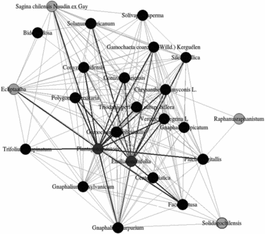
The constellation analysis, or network analysis, involves consolidation of calculation-relevant parameters specific for neighbour plant species with some kind of relationship into a community (Borsboom and Cramer, Reference Borsboom and Cramer2013). It was obtained from an adjacency matrix by using the Fruchterman–Reingold layout definitions, which determines the position of the nodes into the graph (Fruchterman and Reingold, Reference Fruchterman and Reingold1991). The constellation was simplified by an automated process to remove loops and/or multiple edges. This analysis was executed into the R environment with functions made available by the package ‘igraph’, and considering the same limitations proposed by Borsboom and Cramer (Reference Borsboom and Cramer2013). Traits which are less associated to the others are presented on the periphery of the constellation. The constellation analysis constitutes an optional step for studies of plant association. Herein, it was used with the sole aim of validating the associations determined by the χ 2-test, and there should be no need to execute it in studies of plant associations into arable fields. The χ 2-based test should be enough to validate the possible associations.
RESULTS AND DISCUSSION
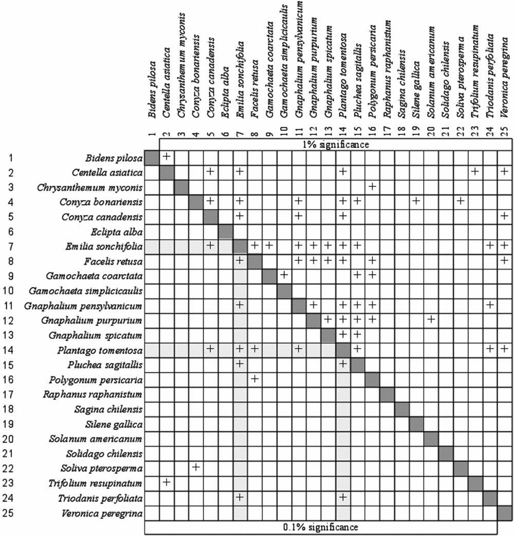
The contingency matrix indicated possibility of association between several pairs of weed species (Figure 1). At 1% significance, 51 associations were reported out of 300 possible associations (17% association possibility). At 0.1% significance, 4.7% of association possibility was reported (14 out of 300). The species that did not associate to any other (1% significance) were Eclipta alba, Raphanus raphanistrum, Sagina chilensis, and Solidago chilensis. On the other hand, the most sociable species were Emilia sonchifolia and Plantago tomentosa, which were able to associate to other six species even at 0.1% significance (Supplementary Figure S1, available online at https://doi.org/10.1017/S0014479718000029).
Complete chi-square contingency matrix for a pool of 100 samples, showing the relationships between pairs of broad-leaved weed species, at 1% and 0.1% significance levels. The species association tree for E. sonchifolia and P. tomentosa are highlighted at the 0.1% significance side of the table.

The χ 2-test, when significant, does not necessarily indicate that the presence of one of these species causes the occurrence of its associates (Herben et al., Reference Herben, Tackenberg and Klimešová2016). However, it reports that the positively associated weed species occur together more often than would be expected by chance (Voinov et al., Reference Voinov, Nikulin and Balakrishnan2013). Among the factors which could favour these positive associations are as follows: (1) similar demand for environmental resources (Gurevitch et al., Reference Gurevitch, Scheiner and Fox2009); (2) frequently imposed selection pressure which causes survival of a given group of independent plants; and (3) interdependence between species, where a factor connected to a given species increases the survival or occurrence of other (Herben et al., Reference Herben, Tackenberg and Klimešová2016). For (1), areas which are too large are most prone to the lack of homogeneity all along its extension; thus, clusters of species which present similar nutrient or moisture demand, as example, tend to naturally occur together with no direct relationships among the species into the cluster (Barbour et al., Reference Barbour, Burk and Pitts1998). The same is observed for small and too inhomogeneous areas. For (2), a frequently imposed selection pressure as the repetitive application of a given herbicide or frequent soil tillage with the same equipment at the same soil depth would naturally select plant species less susceptible to that stress; thus, an ecologically unrelated and independent group of plant species could often occur together while no dependence among species is established. For (3), a root exudate from a given species could promote the germination of seed of a positively associated weed species; the same would be observed in the case where one of the species attracts pollinators which will also pollinate its associates (Imperatriz-Fonseca et al., Reference Imperatriz-Fonseca, Saraiva and Jong2006).
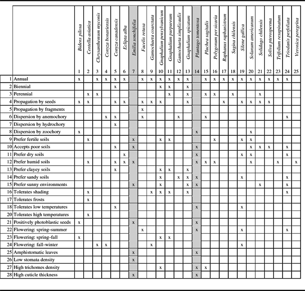
The main plant traits for all weed species that presented some type of association to others (according to Figure 1) are presented in Table 1. It can be seen that the associated species, as schematics in Figure S1, usually have a greater number of intrinsic ecological traits. E. sonchifolia and P. tomentosa presented 8 and 12 remarkable ecological traits, respectively (Table 1). The same occurs for C. canadensis and G. pensylvanicum, with 9 and 10 remarkable ecological traits. Among the common traits to E. sonchifolia and P. tomentosa, three of them are present in some of the other associated species (Table 1): adaptation to poor soils, and preference for humid and sunny environments. These two weed species were the pillars of the overall association (Figure S1) and also were the only ones to present thick cuticle layer on leaves, remarkably amphistomatic, and also positively photoblastic seeds, along with B. pilosa (Table 1).
Most notable plant traits, as cited in the specialized literature, of the weed species included in the study.

Note: Plant species traits present are only the main ones associated to each weed species.
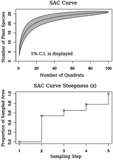
The SAC indicated that at least 25 quadrats (with 0.5-m side) would require sampling to provide a reliable inference about weed occurrence (Figure 2). When evaluating weed occurrence in these fields by using the phytosociological approach (Adegas et al., Reference Adegas, Oliveira, Vieira, Prete, Gazziero and Voll2010; Jakelaitis et al., Reference Jakelaitis, Ferreira, Silva, Agnes, Miranda and Machado2003; Tuffi-Santos et al., Reference Tuffi-Santos, Santos, Oliveira, Santos, Ferreira and Queiroz2004), an unbiased sampling by randomly launching 25 quadrats would supposedly be enough. Although the SAC indicated that 25 quadrats would be enough for a reliable sampling, the SAC steepness (z), which is an indicator of beta diversity, showed that the first quantile of the data was reached by sampling about 50% of the area (corresponding to about 50 quadrats). Thus, the area to be sampled for ecological studies of weed associations should be of at least 13 m2, under equivalent infestation and ecological conditions to the one in the present study, with quadrats randomly distributed.
SAC curve and SAC curve steepness as function of the number of sampled quadrats (and as consequence the sampled area), and the sampling step (quantiles).

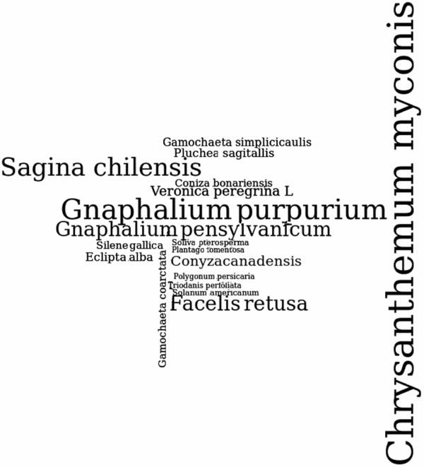
Regarding the overall proportion of species occurrence, C. myconis was the preponderant one, followed by G. purpureum, S. chilensis, F. retusa, and G. pensylvanicum (Figure 3). The remaining species (20 in total) occurred in smaller proportions. It should be noted, however, that there seems to be an inverse relationship between the association potential and the level of occurrence of these weeds in terms of frequency. With exception of F. retusa, the other associated species (Figure S1) occurred only in low levels (Figure 3), which indicates that association is important for survival in unfavourable environments (Dekker, Reference Dekker2009), but that the preponderant weed species are specialized ones, highly aggressive, which turns them into most competitive (Aldrich, Reference Aldrich1984) for environmental resources. Species dependent on associations to other plants for survival seem not to be competitive weeds, but to present mainly ruderal behaviour (Monquero, Reference Monquero2014). When considering the results of the constellation analysis (Figure 4), those species that were not associated to any other in the analysis by the χ 2-test (Figure 1) were located in the periphery of the constellation, being also among the less frequent ones (Figure 3), although with a relatively different overall association tree.
The wordcloud of occurrence of weeds in the sampled field. The occurrence level of the species is proportional to the font size adopted. Extremely rare species (those which were reported in five or less quadrats) were automatically excluded from the analysis.

Constellation analysis by using the Fruchterman–Reingold layout. Weed species represented by a gray circle were not associated to any other species according to the χ 2-test.

CONCLUSIONS
Our study supplies evidence that the hypothesis of plant association aiming survival in arable fields is valid. In general, the plant association technique seems to be appropriate for studies in weed science. Both the χ 2-based test and the constellation analysis, although with distinct groups, were able to indicate those weed species that were not associated to their neighbours. The χ 2-based test should be enough to validate the possible associations, and should be given preference due to easiness of execution and comprehension. The knowledge about plant species associations would allow management strategies to give preference for those herbicides that are efficient on most species into the cluster, in despite of those herbicides controlling only the dominant weed species. This will help reducing the long-term weed selection in arable fields and contribute to the sustainability of herbicide applications.
SUPPLEMENTARY MATERIAL
To view supplementary material for this article, please visit https://doi.org/10.1017/S0014479718000029