



1 Introduction
Among the difficulties arising in the investigation of turbulent free flows, the effects of confinement present an important challenge. This aspect, which will be referred to as saturation in the following, is particularly relevant for the analysis of the well-known test case of free decay of homogeneous isotropic turbulence (HIT). In the spectral space, HIT dynamics can be described by the Lin equation:
 $$\begin{eqnarray}\frac{\unicode[STIX]{x2202}E(k,t)}{\unicode[STIX]{x2202}t}+2\unicode[STIX]{x1D708}k^{2}E(k,t)=T(k,t),\end{eqnarray}$$
where
 $E(k,t)$
is the energy spectrum and
 $T(k,t)$
is the nonlinear energy transfer;
 $\unicode[STIX]{x1D708}$
is the molecular viscosity of the fluid,
 $k$
represents the spectral wavenumber and
 $t$
is the evolution time. The resulting decay regime is determined by a power-law time evolution of the main physical quantities, such as the turbulent kinetic energy
 ${\mathcal{K}}$
, the energy dissipation rate
 $\unicode[STIX]{x1D700}$
, the integral length scale
 $L$
and the Reynolds number
 $Re_{T}=\sqrt{2/3{\mathcal{K}}}L/\unicode[STIX]{x1D708}$
. Considering an unbounded spectral space, the power-law exponent
 $n_{Q}$
driving the time evolution of a general quantity
 $Q$
is determined by the turbulence production mechanisms/initial conditions prescribed (George Reference George1992, Reference George2012; Meldi & Sagaut Reference Meldi and Sagaut2013a
). By the use of theoretical analysis, Comte-Bellot & Corrsin (Reference Comte-Bellot and Corrsin1966) expressed
 $n_{{\mathcal{K}}}$
as an algebraic function of the parameter
 $\unicode[STIX]{x1D70E}$
, which describes the slope of the energy spectrum at the large scales
 $E(k,t)\propto Ak^{\unicode[STIX]{x1D70E}},\unicode[STIX]{x1D70E}\in [1,4]$
. Confinement effects make more complex the description of HIT decay. In fact, in a bounded domain, the growth of the characteristic scales will eventually lead to saturation (i.e. when
 $L$
is as large as the domain typical size, resulting in a constant integral scale decay regime) after a finite time. Extending the analysis by Comte-Bellot & Corrsin (Reference Comte-Bellot and Corrsin1966) to a finite spectral space, Stalp, Skrbek & Donnelly (Reference Stalp, Skrbek and Donnelly1999), Skrbek & Stalp (Reference Skrbek and Stalp2000) showed that the case
 $\unicode[STIX]{x1D70E}=+\infty$
corresponds to complete saturation. The resulting formulae for the main HIT statistical quantities are summarised in table 1.
Analytical formulae for the prediction of the power-law exponents of the decay of the main HIT statistical quantities. The high
 $Re_{\unicode[STIX]{x1D706}}$
formulae are proposed by Comte-Bellot & Corrsin (Reference Comte-Bellot and Corrsin1966) and revisited by Meldi & Sagaut (Reference Meldi and Sagaut2012). The coefficient
 $a=\max (0,0.65\times (\unicode[STIX]{x1D70E}-3.2))$
represents the effects of non-local triadic interactions. The formulae accounting for complete saturation were provided by Skrbek & Stalp (Reference Skrbek and Stalp2000).

While previous studies considered unbounded/completely saturated HIT, the systematic analysis of confinement effects in the transition region between the two asymptotic phenomena, which is the most realistic configuration, is still unexplored. Qualitative elements of discussion have been proposed by Davidson (Reference Davidson2004) and, very recently, by Thornber (Reference Thornber2016). The exclusion of confinement effects is problematic for both experimental analysis and numerical simulation. Due to the limits in size of wind tunnel facilities, the analysis of grid turbulence at high Reynolds number configurations in an unbounded space is a prohibitive task. In fact, anisotropy effects influence HIT evolution in the near grid region, while finite Reynolds number (FRN) effects and saturation govern turbulence dynamics downstream. As a result, quasi-isotropic turbulence for
 $Re_{\unicode[STIX]{x1D706}}>100$
can be observed over a very limited time window, not more than 10–100 initial turnover times
 $t_{0}={\mathcal{K}}(0)/\unicode[STIX]{x1D700}(0)$
(Mohamed & LaRue Reference Mohamed and Larue1990; Mydlarski & Warhaft Reference Mydlarski and Warhaft1996; White, Karpetis & Sreenivasan Reference White, Karpetis and Sreenivasan2002; Krogstad & Davidson Reference Krogstad and Davidson2011; Thormann & Meneveau Reference Thormann and Meneveau2014; Sinhuber, Bodenschatz & Bewley Reference Sinhuber, Bodenschatz and Bewley2015).
 $Re_{\unicode[STIX]{x1D706}}=\sqrt{2/3{\mathcal{K}}}\unicode[STIX]{x1D706}/\unicode[STIX]{x1D708}=\sqrt{20/3Re_{T}}$
is the Reynolds number based on the Taylor microscale
 $\unicode[STIX]{x1D706}$
. Direct numerical simulation (DNS) suffers similar drawbacks. Presently, the computational resources available impose very strict constraints for the analysis of HIT free decay. The resolution at the large scales progressively decreases in time as the integral length scale
 $L$
increases, so that a smaller initial
 $Re_{\unicode[STIX]{x1D706}}$
has to be imposed if longer observation times are required. This aspect is particularly complex to handle for classical numerical simulation, as the resolution at the large scales diminishes significantly in the time needed for a statistically converged observation. Ishida, Davidson & Kaneda (Reference Ishida, Davidson and Kaneda2006) performed a comprehensive analysis by DNS and indicated a minimum resolution of one decade at the large scales at the final time in order to avoid saturation effects. However, the analysis was based on observations for initial values of the Reynolds number in the range
 $250>Re_{\unicode[STIX]{x1D706}}(0)>31.3$
. Recent experimental studies by Djenidi, Kamruzzamana & Antonia (Reference Djenidi, Kamruzzamana and Antonia2015) show that finite Reynolds number effects are not negligible for
 $Re_{\unicode[STIX]{x1D706}}\leqslant 100$
, so that extrapolation towards high Reynolds number turbulence is questionable. Arguably, saturation effects play an important role in the lack of agreement between theoretical studies, experimental results and numerical simulations reported in the open literature.
In the present paper, the confinement effects before the fully saturated regime at high Reynolds number configurations are analysed via a theoretical study and eddy-damped quasi-normal Markovian (EDQNM) calculation (Orszag Reference Orszag1970). In both cases, a fixed resolution at the large scales is imposed i.e. the saturation threshold and the integral length scale
 $L$
follow the same time evolution. In this way, saturation effects can be isolated and quantified over long observation times, which are precluded in classical experimental and numerical analyses. The constant resolution at the large scales is numerically obtained by the use of the recent model proposed by Meldi & Sagaut (Reference Meldi and Sagaut2014), which resolves the EDQNM problem over an adaptive spectral mesh.
The paper is structured as follows. In § 2, saturation effects are isolated in the framework of an energy spectrum analysis. In § 3, numerical details about the model and the set-up of the simulations are provided. In § 4, the effects of saturation are investigated. In § 5, the theoretical/EDQNM results are elaborated in order to estimate confinement effects in DNS and experiments. Finally, in § 6, the final remarks are drawn.
2 Confinement effects in the unsaturated regime: a theoretical analysis
The effects of large-scale confinement over quasi-unbounded regimes in a bounded box are now investigated through theoretical analysis. The present work elaborates on the proposals by Comte-Bellot & Corrsin (Reference Comte-Bellot and Corrsin1966) and Skrbek, Niemela & Donnelly (Reference Skrbek, Niemela and Donnelly2000), Skrbek & Stalp (Reference Skrbek and Stalp2000). The first work addresses the case of unbounded regimes while the latter investigates completely saturated regimes. The present analysis aims at deriving information for the range of configurations between the two asymptotic regimes. Here the spectrum at the large scales is not neglected, but its size is finite and constant through the time evolution. A simplified energy spectrum as in figure 1 is used as a starting point:
 $$\begin{eqnarray}E(k,t)=\left\{\begin{array}{@{}ll@{}}0\quad & k<\unicode[STIX]{x1D6FC}k_{L}(t)\\ Ak^{\unicode[STIX]{x1D70E}}\quad & \unicode[STIX]{x1D6FC}k_{L}(t)\leqslant k\leqslant k_{L}(t)\\ C_{K}\unicode[STIX]{x1D700}^{2/3}(t)k^{-5/3}\quad & k_{L}(t)<k\leqslant k_{\unicode[STIX]{x1D702}}(t)\\ 0\quad & k>k_{\unicode[STIX]{x1D702}}(t),\end{array}\right.\end{eqnarray}$$
where
 $k_{L}(t)=1/L(t)$
and
 $k_{\unicode[STIX]{x1D702}}(t)=1/\unicode[STIX]{x1D702}(t)$
are the wavenumbers associated with the integral length scale
 $L$
and the Kolmogorov scale
 $\unicode[STIX]{x1D702}$
, respectively. They relate as
 $k_{\unicode[STIX]{x1D702}}=Re_{T}^{3/4}k_{L}$
.
 $C_{K}=1.5$
is the Kolmogorov constant and the parameter
 $A$
can be derived considering the continuity constraint of the energy spectrum at
 $k_{L}$
:
 $A^{3}k_{L}^{3\unicode[STIX]{x1D70E}+5}=C_{K}^{3}\unicode[STIX]{x1D700}^{2}$
. The constant
 $\unicode[STIX]{x1D6FC}$
represents the resolution at the large scales. More precisely,
 $\unicode[STIX]{x1D6FC}k_{L}(t)$
and
 $k_{L}(t)$
evolve following the same power law, so that the resolution at the large scales is hypothesised as constant. Thus, a physical system described by the energy spectrum in (2.1) would grow in space with the same time evolution of the integral length scale
 $L$
. Such an approximation is here used to investigate the effect of a constant confinement for very long observation times, so that a converged statistical behaviour can be quantified. Moreover, a time evolution of the parameter
 $A(t)=\overline{A}k_{L}^{-a}(t)$
is considered (Eyink & Thomson Reference Eyink and Thomson2000; Meldi & Sagaut Reference Meldi and Sagaut2012). The value of the parameter
 $a=\max (0,0.65\times (\unicode[STIX]{x1D70E}-3.2))$
is connected with the fulfilment of the permanence of large eddies hypothesis.
Time evolution of the energy spectrum introduced in (2.1).

If the spectrum in (2.1) is integrated, the following expression for
 ${\mathcal{K}}$
is obtained:
 $$\begin{eqnarray}{\mathcal{K}}=\left[\frac{\overline{A}k^{\unicode[STIX]{x1D70E}-a+1}}{\unicode[STIX]{x1D70E}-a+1}\right]_{\unicode[STIX]{x1D6FC}k_{L}}^{k_{L}}+\left[-\frac{3}{2}C_{K}\unicode[STIX]{x1D700}^{2/3}k^{-2/3}\right]_{k_{L}}^{k_{\unicode[STIX]{x1D702}}}.\end{eqnarray}$$
Using the continuity constraint of the spectrum at
 $k=k_{L}$
,
 $k_{L}$
and
 $k_{\unicode[STIX]{x1D702}}$
are elaborated to obtain an expression of
 ${\mathcal{K}}={\mathcal{K}}(\overline{A},C_{K},\unicode[STIX]{x1D70E},Re_{T},\unicode[STIX]{x1D6FC},\unicode[STIX]{x1D700})$
:
 $$\begin{eqnarray}{\mathcal{K}}=[B-C]D\unicode[STIX]{x1D700}^{2((\unicode[STIX]{x1D70E}-a+1)/(3(\unicode[STIX]{x1D70E}-a)+5))},\end{eqnarray}$$
where
 $$\begin{eqnarray}\left.\begin{array}{@{}c@{}}\displaystyle B=\frac{3(\unicode[STIX]{x1D70E}-a)+5}{2(\unicode[STIX]{x1D70E}-a+1)},\quad C=\left(\frac{\unicode[STIX]{x1D6FC}^{\unicode[STIX]{x1D70E}-a+1}}{\unicode[STIX]{x1D70E}-a+1}+\frac{3}{2Re_{T}^{1/2}}\right),\\ \displaystyle D=\overline{A}^{2/(3(\unicode[STIX]{x1D70E}-a)+5)}C_{K}^{3((\unicode[STIX]{x1D70E}-a+1)/(3(\unicode[STIX]{x1D70E}-a)+5))}.\end{array}\right\}\end{eqnarray}$$
The Lin equation (1.1) is now integrated over
 $k$
, yielding:
 $$\begin{eqnarray}\frac{\unicode[STIX]{x2202}{\mathcal{K}}}{\unicode[STIX]{x2202}t}+\unicode[STIX]{x1D700}=\unicode[STIX]{x0394}T,\end{eqnarray}$$
where
 $\unicode[STIX]{x0394}T=0$
in the case of full resolution of all the dynamically active scales of HIT. Equation (2.5) is now elaborated imposing a power-law solution of the form
 $\unicode[STIX]{x1D700}=\unicode[STIX]{x1D700}_{0}(1+t/t_{0})^{n_{\unicode[STIX]{x1D700}}}$
. As a consequence, the right-hand term must exhibit the same power-law evolution, which will be modelled as
 $\unicode[STIX]{x0394}T=\unicode[STIX]{x0394}T_{0}(1+t/t_{0})^{n_{\unicode[STIX]{x1D700}}}$
:
 $$\begin{eqnarray}\displaystyle & & \displaystyle (B-C)D\left(2\frac{\unicode[STIX]{x1D70E}-a+1}{3(\unicode[STIX]{x1D70E}-a)+5}\right)n_{\unicode[STIX]{x1D700}}\frac{\unicode[STIX]{x1D700}_{0}^{2((\unicode[STIX]{x1D70E}-a+1)/(3(\unicode[STIX]{x1D70E}-a)+5))}}{t_{0}}\left(1+\frac{t}{t_{0}}\right)^{n_{\unicode[STIX]{x1D700}}}+\unicode[STIX]{x1D700}_{0}\left(1+\frac{t}{t_{0}}\right)^{n_{\unicode[STIX]{x1D700}}}\nonumber\\ \displaystyle & & \displaystyle \quad =\unicode[STIX]{x0394}T_{0}\left(1+\frac{t}{t_{0}}\right)^{n_{\unicode[STIX]{x1D700}}}.\end{eqnarray}$$
In the case of fully resolved high Reynolds HIT, the value of the constants tend to
 $\unicode[STIX]{x1D6FC}\rightarrow 0$
,
 $Re_{T}\rightarrow +\infty$
and
 $\unicode[STIX]{x0394}T_{0}\rightarrow 0$
. Thus,
 $C=0$
and the result by Comte-Bellot & Corrsin (Reference Comte-Bellot and Corrsin1966) analysis in table 1 is recovered. Equation (2.6) is now divided by
 $(1+t/t_{0})^{n_{\unicode[STIX]{x1D700}}}$
. The following expression for
 $n_{\unicode[STIX]{x1D700}}$
is derived:
 $$\begin{eqnarray}\displaystyle n_{\unicode[STIX]{x1D700}} & = & \displaystyle \frac{3(\unicode[STIX]{x1D70E}-a)+5}{2(\unicode[STIX]{x1D70E}-a+1)}t_{0}\frac{\unicode[STIX]{x0394}T_{0}-\unicode[STIX]{x1D700}_{0}}{(B-C)D\unicode[STIX]{x1D700}_{0}^{2((\unicode[STIX]{x1D70E}-a+1)/(3(\unicode[STIX]{x1D70E}-a)+5))}}\nonumber\\ \displaystyle & = & \displaystyle -\frac{3(\unicode[STIX]{x1D70E}-a)+5}{2(\unicode[STIX]{x1D70E}-a+1)}\frac{t_{0}\unicode[STIX]{x1D700}_{0}^{(\unicode[STIX]{x1D70E}-a+3)/(3(\unicode[STIX]{x1D70E}-a)+5)}}{BD}(1+{\mathcal{F}})=n_{\unicode[STIX]{x1D700}}^{\star }(1+{\mathcal{F}})\end{eqnarray}$$
 $n_{\unicode[STIX]{x1D700}}^{\star }$
is the power-law exponent obtained by the Comte-Bellot & Corrsin analysis. The expression for
 $n_{\unicode[STIX]{x1D700}}^{\star }$
in (2.7) can be elaborated to obtain the result in table 1, using underlying relations between the parameters describing the energy spectrum and
 $\unicode[STIX]{x1D700}_{0}$
,
 $t_{0}$
. On the other hand,
 ${\mathcal{F}}(\unicode[STIX]{x1D6FC},Re_{T},\unicode[STIX]{x0394}T_{0})$
is a correction function which accounts for saturation and finite Reynolds number effects. Further manipulation of (2.7) gives the expression:
 $$\begin{eqnarray}{\mathcal{F}}=\frac{C-B\unicode[STIX]{x0394}T_{0}\unicode[STIX]{x1D700}_{0}^{-1}}{B-C}=\frac{2\unicode[STIX]{x1D6FC}^{\unicode[STIX]{x1D70E}-a+1}+3(\unicode[STIX]{x1D70E}-a+1)Re_{T}^{-1/2}-(3(\unicode[STIX]{x1D70E}-a)+5)\unicode[STIX]{x0394}T_{0}\unicode[STIX]{x1D700}_{0}^{-1}}{3(\unicode[STIX]{x1D70E}-a)+5-2\unicode[STIX]{x1D6FC}^{\unicode[STIX]{x1D70E}-a+1}-3(\unicode[STIX]{x1D70E}-a+1)Re_{T}^{-1/2}}.\end{eqnarray}$$
Considering the relation
 $n_{\unicode[STIX]{x1D700}}=n_{{\mathcal{K}}}-1$
, equation (2.7) can be rewritten with the same formalism for the power-law exponent
 $n_{{\mathcal{K}}}$
. The analysis of (2.7)–(2.8) indicates that saturation is responsible for a faster decay of
 $\unicode[STIX]{x1D700}$
and
 ${\mathcal{K}}$
. The same conclusion can be drawn for finite Reynolds number effects. On the other hand, the contribution of the term
 $\unicode[STIX]{x0394}T_{0}\unicode[STIX]{x1D700}_{0}^{-1}$
can be either positive or negative. Considering saturation effects only (i.e.
 $\unicode[STIX]{x0394}T_{0}=0,Re_{T}\rightarrow +\infty$
), one can observe that
 ${\mathcal{F}}\propto \unicode[STIX]{x1D6FC}^{\unicode[STIX]{x1D70E}-a+1}$
, so that the magnitude of the power-law exponent evolves towards the fully saturated value as
 $\unicode[STIX]{x1D6FC}$
increases. This last result implies as well that (2.8) can be well approximated by a power-law function of the parameter
 $\unicode[STIX]{x1D6FC}$
. However, for
 $\unicode[STIX]{x1D6FC}\rightarrow 1$
,
 ${\mathcal{F}}$
is expected to exhibit a progressively slower evolution. In fact, the slope of the energy spectrum evolves from the value
 $\unicode[STIX]{x1D70E}$
to the value
 $-5/3$
over approximately a decade in the spectral space
 $k$
for a realistic configuration (see figure 4
a).
3 The EDQNM model
A brief summary about the numerical details of the EDQNM model is now provided. A comprehensive analysis is reported in the works by Orszag (Reference Orszag1970), Sagaut & Cambon (Reference Sagaut and Cambon2008). The model is based on the Lin equation (1.1), which describes the time evolution of the energy spectrum in HIT decay. The EDQNM closure operates in the evolution equation for
 $T(k,t)$
. The fourth-order cumulants, which measure the difference between the actual velocity probability density function (PDF) from a Gaussian distribution, are modelled as a linear damping term. Moreover, the characteristic dissipation time is neglected with respect to the evolution time through the Markovian approximation. These two hypotheses produce a dramatic simplification in the evolution equation for
 $T(k,t)$
:
 $$\begin{eqnarray}T_{EDQNM}(k,t)=\int _{p+q=k}\unicode[STIX]{x1D6E9}_{kpq}(xy+z^{3})E(p,t)[E(p,t)pk^{2}-E(k,t)p^{3}]\frac{\text{d}p\,\text{d}q}{pq},\end{eqnarray}$$
where
 $x$
,
 $y$
,
 $z$
are geometrical coefficients associated with the spherical integration in the spectral space and
 $\unicode[STIX]{x1D6E9}_{kpq}$
is the characteristic time of relaxation recovered by the Markovianisation procedure. In the present work, the adaptive formulation by Meldi & Sagaut (Reference Meldi and Sagaut2014) is used to update the spectral mesh, which is defined by a geometrical distribution. The EDQNM equations are not modified, but a dynamic mesh calculation is implemented. This procedure allows one to prescribe a fixed large-scale/small-scale resolution. In the present analysis, the adaptive procedure conserves the total number of elements
 $N$
and imposes a fixed ratio
 $k_{L}(t)/k_{1}(t)=\unicode[STIX]{x1D6FC}^{-1}$
. Energy conservation through the dynamic mesh update is obtained using the following definition of
 ${\mathcal{K}}$
:
 $$\begin{eqnarray}{\mathcal{K}}(t)=\int _{0}^{k_{1}}Ak^{\unicode[STIX]{x1D70E}}\,\text{d}k+\int _{k_{1}}^{k_{N}}E(k,t)\,\text{d}k=A_{{\mathcal{K}}}+\int _{k_{1}}^{k_{N}}E(k,t)\,\text{d}k,\end{eqnarray}$$
where
 $k_{1}$
and
 $k_{N}$
are the smallest and largest resolved mode, respectively. The coefficient
 $A_{{\mathcal{K}}}$
is updated every time the mesh is adapted (i.e. smaller/larger elements are introduced), in order to conserve the total energy
 ${\mathcal{K}}$
. More precisely, the resolution at the large scales is checked at the beginning of each time step. Whenever
 $k_{L}(t)/k_{1}(t)<\unicode[STIX]{x1D6FC}^{-1}$
, the mesh is updated so that
 $k_{j}(t^{\ast })=k_{j}(t)/r_{s}$
. Where
 $r_{s}$
is the ratio of the geometrical distribution of the mesh elements and
 $t$
and
 $t^{\ast }$
represent the same time step, but they are defined as the time before/after the adaptive procedure, respectively. Additionally, the constant
 $A_{{\mathcal{K}}}$
is updated using the integral in (3.2):
 $A_{{\mathcal{K}}}(t^{\ast })=\int _{0}^{k_{1}(t^{\ast })}Ak^{\unicode[STIX]{x1D70E}}\,\text{d}k$
. In this way, the turbulent kinetic energy and all the other physical quantities investigated are exactly conserved through
 $t\rightarrow t^{\ast }$
. However,
 $A_{{\mathcal{K}}}$
does not play a role in the numerical computation of the EDQNM closure, which is performed on the spectral mesh
 $k_{1},\ldots ,k_{N}$
. While the adaptive EDQNM calculation does not use the energy spectrum in (2.1), it captures the essential feature of the theoretical model proposed in § 2, which is a constant large-scale resolution during HIT decay. The time evolution of all HIT statistical moments is calculated by the EDQNM procedure and is not affected by the mesh time evolution (Meldi & Sagaut Reference Meldi and Sagaut2014). The nonlinear energy transfer budget term
 $kT(k,t)$
at the beginning/end of a time step where the adaptive procedure is triggered is shown in figure 2. In the present analysis, a constraint is imposed for the large scales only, and the total number of mesh elements
 $N$
is conserved. As a consequence, the small-scale resolution increases in time from the initial value
 $k_{N}(0)/k_{\unicode[STIX]{x1D702}}(0)$
as
 $Re_{T}$
decreases.
Nonlinear energy transfer budget term
 $kT(k,t)$
at the beginning and at the end of a time step for which the mesh adaptive procedure is triggered. Data are taken from simulation 1 of the Saffman database, where the condition
 $\unicode[STIX]{x1D6FC}=10^{-1/30}$
is imposed.

The present work encompasses the analysis of energy statistical quantities and their pressure counterparts. The pressure spectrum
 $E_{p}$
is derived by the EDQNM model using the integration method proposed by Lesieur, Ossia & Metais (Reference Lesieur, Ossia and Metais1999), Meldi & Sagaut (Reference Meldi and Sagaut2013b
) through the joint Gaussian assumption:
 $$\begin{eqnarray}E_{p}(k,t)=\frac{k^{2}}{4\unicode[STIX]{x03C0}}\int _{p+q=k}E(p,t)E(q,t)\frac{\sin ^{4}\unicode[STIX]{x1D709}}{p^{4}}\,\text{d}q,\end{eqnarray}$$
where
 $[k,p,q]$
is the basis used to compute the triadic interactions and
 $\unicode[STIX]{x1D709}$
is the angle facing
 $p$
in the triangle formed by the three vectors of the basis. The statistical quantities analysed are:
-
(i) turbulent kinetic energy
 ${\mathcal{K}}(t)=\int _{0}^{+\infty }E(k,t)\,\text{d}k$
;
-
(ii) energy dissipation rate
$\unicode[STIX]{x1D700}(t)=\int _{0}^{+\infty }2\unicode[STIX]{x1D708}k^{2}E(k,t)\,\text{d}k$
; -
(iii) integral length scale
$L(t)=(3\unicode[STIX]{x03C0}/4)((\int _{0}^{+\infty }k^{-1}E(k,t)\,\text{d}k)/(\int _{0}^{+\infty }E(k,t)\,\text{d}k))$
; -
(iv) turbulence coefficient
$C_{\unicode[STIX]{x1D700}}(t)=\sqrt{27/8}L(t)\unicode[STIX]{x1D700}(t)/{\mathcal{K}}^{3/2}(t)$
; -
(v) pressure fluctuation variance
$\overline{p^{2}}(t)=\int _{0}^{+\infty }E_{p}(k,t)\,\text{d}k$
; -
(vi) velocity derivative skewness
$S(t)=-(3\sqrt{30}/14)((\int _{k_{1}}^{k_{N}}k^{2}T(k,t)\,\text{d}k)/((\int _{k_{1}}^{k_{N}}k^{2}E(k,t)\,\text{d}k)^{3/2}))$
; -
(vii) coefficient of the
$4/5$
Kolmogorov law
$C_{3}=-\max \,S_{3}(r)/(\unicode[STIX]{x1D700}r)$
.








Here
 $S_{3}=\langle (\unicode[STIX]{x1D6FF}u_{L})^{3}\rangle$
is the statistical third-order moment of the velocity increment along the separation vector
 $(r)$
of modulus
 $r$
.
3.1 Numerical set-up
The effects of saturation have been investigated by the use of two databases of EDQNM simulations. More precisely, the investigation is performed for the cases of Saffman turbulence (
 $\unicode[STIX]{x1D70E}=2$
) and Batchelor turbulence (
 $\unicode[STIX]{x1D70E}=4$
). Each database is composed by a total of 60 simulations, which are initialised prescribing the following functional form:
 $$\begin{eqnarray}E(k)=C_{k}\unicode[STIX]{x1D700}^{2/3}k^{-5/3}f_{L}(kL)f_{\unicode[STIX]{x1D702}}(k\unicode[STIX]{x1D702}),\end{eqnarray}$$
with:
 $$\begin{eqnarray}f_{L}(kL)=\left(\frac{kL}{[(kL)^{3/2}+c_{L} )]^{2/3}}\right)^{5/3+\unicode[STIX]{x1D70E}},\quad f_{\unicode[STIX]{x1D702}}(k\unicode[STIX]{x1D702})=\exp (-\unicode[STIX]{x1D709}([(k\unicode[STIX]{x1D702})^{4}+c_{\unicode[STIX]{x1D702}}^{4}]^{1/4}-c_{\unicode[STIX]{x1D702}})),\end{eqnarray}$$
where
 $c_{\unicode[STIX]{x1D702}}=0.4$
,
 $\unicode[STIX]{x1D709}=5.3$
and
 $c_{L}$
has been chosen to obtain
 $L(0)=1$
. The initial Reynolds number is
 $Re_{\unicode[STIX]{x1D706}}(0)=1.5\times 10^{5}$
. For every numerical simulation, the initial value of the largest resolved mode has been chosen as
 $k_{N}(0)/k_{\unicode[STIX]{x1D702}}(0)=2$
. The
 $N_{i}$
elements of the spectral mesh are distributed following a geometrical progression so that
 $k_{j+1}/k_{j}=10^{1/30},j=1,2,\ldots ,N-1$
. For the simulation
 $i\in [1,60]$
of the database, the resolution criterion at the large scales has been set so that
 $k_{L}/k_{1}=10^{i/30}$
. Thus, a constant resolution at the large scales in the range zero to two decades in the spectral space is analysed. As introduced in § 3, the adaptive procedure checks the value of
 $k_{L}/k_{1}$
at each time step. Whenever
 $k_{L}(t)/k_{1}<10^{i/30}$
, the mesh and the coefficient
 $A_{{\mathcal{K}}}$
are updated so that
 $k_{j}(t^{\ast })=k_{j}(t)/10^{1/30},j=1,2,\ldots ,N$
. Thus, the mesh slides towards smaller modes as
 $L$
increases in time, in order to conserve the ratio
 $k_{L}/k_{1}\approx \text{const}$
. The initial resolution at the large scales is set to
 $k_{L}/k_{1}=10^{(i+20)/30}$
, so that the adaptive procedure is not triggered during the initial transient. Moreover, as the initial values of
 $Re_{\unicode[STIX]{x1D706}}(0)$
and
 $k_{L}(0)$
are the same for every calculation, the total number of elements
 $N_{i}$
of the spectral mesh linearly increases with the resolution:
 $N_{i}=N_{1}+(i-1)$
. The power-law coefficients of HIT statistical quantities have been computed from data in the range
 $Re_{\unicode[STIX]{x1D706}}=10^{5}\rightarrow 300$
, in order to achieve a full statistical convergence of the results. This corresponds to an observation window of
 $8\rightarrow 25$
time decades, because of the sensitivity of
 $Re_{\unicode[STIX]{x1D706}}$
decay to the resolution criterion imposed and to the initially prescribed value of
 $\unicode[STIX]{x1D70E}$
(see table 1). For all cases, a very smooth behaviour of the power-law coefficients has been observed in the investigated range. In particular, local oscillations of
 $n_{{\mathcal{K}}}$
never exceeded 0.5 % of the average value calculated after a suitable transient, as shown in figure 3.
(a) Time evolution of
 ${\mathcal{K}}$
for simulation 1, 10 and 60 of the database (Saffman turbulence,
 $\unicode[STIX]{x1D70E}=2$
). (b) Power-law exponent
 $n_{{\mathcal{K}}}$
calculated by local polynomial fitting.

The EDQNM database produced with the adaptive method has been compared with classical calculations. For the latter case, fully resolved and fully saturated solutions have been derived. Important differences are highlighted by the comparison of
 $E(k,t)$
and
 $kT(k,t)$
, which are reported in figure 4(a,b). In fact, while the small-scale region is mostly unchanged, saturation effects progressively modify the shape of the spectra in the large-scale region. One important consequence observed is a non-zero energy transfer due to the coarse resolution at the large scales:
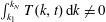 $\int _{k_{1}}^{k_{N}}T(k,t)\,\text{d}k\neq 0$
. This aspect will be investigated in detail in § 4. Moreover, the most saturated case investigated in the database, i.e.
 $\unicode[STIX]{x1D6FC}=10^{-1/30}$
, shows characteristics that are intermediate between the fully resolved case and the fully saturated counterpart. Thus, one can expect to observe a progressive change of the behaviour of HIT physical quantities while saturation effects become more important. At the same time, the observation of figure 4 suggests that the fully saturated statistics (and in particular
 $n_{{\mathcal{K}}}=-2$
) should not be observed in the database of adaptive EDQNM simulations. The same conclusion can be drawn by the analysis of (2.8). In fact, considering
 $\unicode[STIX]{x0394}T_{0}=0$
,
 $Re_{T}\rightarrow \infty$
and
 $\unicode[STIX]{x1D6FC}=1$
, the analytical values of the power-law exponent calculated using (2.7) are
 $n_{{\mathcal{K}}}\approx -1.42$
and
 $n_{{\mathcal{K}}}\approx -1.53$
for Saffman and Batchelor turbulence, respectively. These values are significantly smaller in magnitude when compared to the fully saturated case
 $n_{{\mathcal{K}}}=-2$
.
(a) Energy spectra
 $E(k,t)$
and (b) energy transfer budget term
 $kT(k,t)$
for different resolution at the large scales, calculated by the use of an EDQNM model. The Reynolds number is here
 $Re_{\unicode[STIX]{x1D706}}=10^{3}$
.

4 Results
The numerical results obtained by the adaptive EDQNM model are presented in the following. The effects of saturation over the energy transfer are first investigated. In figure 4, saturation modifies the shape of the energy spectrum in the large-scale region, which results in a non-zero energy transfer in the numerical simulation. A comprehensive analysis of this aspect for the two EDQNM databases is reported in figure 5. Firstly, the relation
 $\unicode[STIX]{x0394}T\propto \unicode[STIX]{x1D700}$
has been observed in all cases. This result, which is exemplified in figure 5(a), is consistent with (2.5). The value of the ratio
 $\unicode[STIX]{x0394}T_{0}/\unicode[STIX]{x1D700}_{0}$
has then been investigated for the databases and the results are shown in figure 5(b). For the case of Saffman turbulence, the term
 $\unicode[STIX]{x0394}T_{0}/\unicode[STIX]{x1D700}_{0}$
is positive, which implies that it contributes to a decrease in magnitude of the power-law exponents. This contribution can be well approximated by the relation
 $\unicode[STIX]{x0394}T_{0}/\unicode[STIX]{x1D700}_{0}\approx 10^{-2}\unicode[STIX]{x1D6FC}^{4.75}$
. Thus, it is negligible when compared to the saturation term
 $2\unicode[STIX]{x1D6FC}^{\unicode[STIX]{x1D70E}+1}=2\unicode[STIX]{x1D6FC}^{3}$
. The value 4.75 in the power-law relation for
 $\unicode[STIX]{x0394}T_{0}/\unicode[STIX]{x1D700}_{0}$
does not appear to have any connection with the physical evolution of HIT, but it is driven by the numerical discretisation of the Lin equation. In DNS, this term could have a significantly higher relevance with respect to
 $\unicode[STIX]{x1D6FC}$
, in particular if the numerical discretisation does not show good properties of conservation of the integral
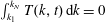 $\int _{k_{1}}^{k_{N}}T(k,t)\,\text{d}k=0$
. The results for the case of Batchelor turbulence are significantly more complex. While
 $\unicode[STIX]{x0394}T_{0}/\unicode[STIX]{x1D700}>0$
for high
 $k_{L}/k_{1}$
values, a change of sign is observed for
 $k_{L}/k_{1}\approx 3$
. Moreover, in this case, the saturation term and the energy transfer error term scale with a similar power law of
 $\unicode[STIX]{x1D6FC}$
. These observations are a result of the high sensitivity of Batchelor turbulence to non-local interaction (Meldi & Sagaut Reference Meldi and Sagaut2012). This feature sets the stage for more complex interactions of the different effects at play.
(a) Evolution of the error in the energy transfer
 $\unicode[STIX]{x0394}T/\unicode[STIX]{x1D700}$
for two simulations of the EDQNM database,
 $k_{L}/k_{1}=10^{1/6},10$
. (b) Sensitivity of the error in the energy transfer
 $\unicode[STIX]{x0394}T/\unicode[STIX]{x1D700}$
to the large-scale resolution
 $k_{L}/k_{1}$
.

4.1 Sensitivity of the large-scale physical quantities to confinement effects
The predicted value of the power-law exponent
 $n_{{\mathcal{K}}}$
is now discussed. The EDQNM results (symbols), along with the theoretical equation (2.7) (solid lines) are reported in figure 6. Each symbol represents an EDQNM calculation of the database for the corresponding value of the parameter
 $\unicode[STIX]{x1D6FC}$
. For the case of Saffman turbulence, the theoretical prediction is not far from the EDQNM observation, and a very good agreement is observed in the range
 $10^{-2}\leqslant \unicode[STIX]{x1D6FC}\leqslant 10^{-1}$
. For lower
 $k_{L}/k_{1}$
values, the complexity of the shape of the energy spectrum at the large scales is responsible for the deviation from the theoretical predictions. This observation is even more true for Batchelor turbulence. One can hypothesise that its sensitivity to non-local interaction amplifies the deviation from the theoretical prediction in (2.7), which is based on a simplification of the shape of the energy spectrum in the peak region.
Sensitivity of
 $n_{{\mathcal{K}}}$
to saturation effects. Theoretical and EDQNM results are shown.

A power-law approximation of the function
 ${\mathcal{F}}$
is now proposed, in order to derive a continuous formulation with respect to
 $\unicode[STIX]{x1D70E}$
. Here, only saturation effects are included. In this case,
 ${\mathcal{F}}$
evolves following a power law of the parameter
 $\unicode[STIX]{x1D6FC}$
. Thus, the approximation proposed is:
 $$\begin{eqnarray}n_{{\mathcal{K}}}=n_{{\mathcal{K}}}^{\star }[1+\overline{{\mathcal{F}}}]=n_{{\mathcal{K}}}^{\star }[1+a_{\unicode[STIX]{x1D70E}}\times \unicode[STIX]{x1D6FC}^{b_{\unicode[STIX]{x1D70E}}}].\end{eqnarray}$$
A constrained optimisation using the EDQNM database is performed, in order to determine the values of the coefficients
 $a_{\unicode[STIX]{x1D70E}}$
and
 $b_{\unicode[STIX]{x1D70E}}$
. The analysis is performed separately for the cases of Saffman and Batchelor turbulence. The two constraints are (i) minimised difference using an
 $L2$
norm between the EDQNM results and the analytical formula (2.8) and (ii) imposing a local difference smaller than 1 % for
 $\unicode[STIX]{x1D6FC}=10^{-1/30}$
. The optimisation results indicate values of the constants equal to
 $a_{2}=0.25$
,
 $b_{2}=1.92$
,
 $a_{4}=0.3$
and
 $b_{4}=2.38$
for Saffman and Batchelor turbulence, respectively. If a linear variation with respect to
 $\unicode[STIX]{x1D70E}$
is hypothesised, the coefficient can be calculated by the following formulae:
 $$\begin{eqnarray}a_{\unicode[STIX]{x1D70E}}=0.2+0.025\times \unicode[STIX]{x1D70E},\quad b_{\unicode[STIX]{x1D70E}}=1.46+0.23\times \unicode[STIX]{x1D70E}.\end{eqnarray}$$
The comparison between the optimised analytical formula (dashed lines) and the power-law exponent derived by the EDQNM data is shown in figure 6. The correspondence between the two curves is good for both Saffman and Batchelor turbulence. The local difference never exceeds 1.5 %. Moreover, the coefficient
 $a_{\unicode[STIX]{x1D70E}}$
can be approximated by
 $a_{\unicode[STIX]{x1D70E}}=-n_{{\mathcal{K}}}^{\star }/4.8$
. Another, less precise approximation is
 $a_{\unicode[STIX]{x1D70E}}\approx 0.5(n_{{\mathcal{K}}}^{\star }-n_{{\mathcal{K}}}(\unicode[STIX]{x1D70E}\rightarrow +\infty ))$
. So,
 $\unicode[STIX]{x1D6FC}=1$
is a sort of intermediate configuration between the fully resolved case and the completely saturated case, in agreement with the qualitative observations of figure 4 and theoretical predictions. Moreover, the observation of the EDQNM results indicate that the classical turbulence relations, such as
 $n_{{\mathcal{K}}}=n_{\unicode[STIX]{x1D700}}+1$
and
 $C_{\unicode[STIX]{x1D700}}\approx \text{constant}$
are well verified even for low resolution at the large scales. In particular, the sensitivity of
 $n_{C_{\unicode[STIX]{x1D700}}}$
to the parameter
 $\unicode[STIX]{x1D6FC}$
is shown in figure 7(a).
 $C_{\unicode[STIX]{x1D700}}$
is an invariant when Kolmogorov theory is verified, while it exhibits a time evolution when turbulence equilibrium is violated (Valente & Vassilicos Reference Valente and Vassilicos2012; Goto & Vassilicos Reference Goto and Vassilicos2015; Meldi Reference Meldi2016). The present results indicate very small, positive values even as
 $\unicode[STIX]{x1D6FC}\rightarrow 0$
. This observation is consistent with previous studies by Bos, Shao & Bertoglio (Reference Bos, Shao and Bertoglio2007) and is associated with the time evolution of the inertial range of
 $E(k,t)$
. This aspect creates an unbalance between the cascade time
 $t_{C}$
and the dissipation time
 $t_{D}$
. A confirmation is given by the higher value of
 $n_{C_{\unicode[STIX]{x1D700}}}$
for Batchelor turbulence, which exhibits a faster decay of
 $Re_{T}$
. On the other hand,
 $n_{C_{\unicode[STIX]{x1D700}}}$
shows a very weak sensitivity for
 $\unicode[STIX]{x1D6FC}\rightarrow 1$
. In particular, the maximum value here observed
 $n_{C_{\unicode[STIX]{x1D700}}}\approx 0.01$
is significantly smaller than the value
 $n_{C_{\unicode[STIX]{x1D700}}}\approx -n_{Re_{T}}$
derived by Goto & Vassilicos (Reference Goto and Vassilicos2015). This result suggests that saturation is not responsible for an anomalous behaviour of
 $C_{\unicode[STIX]{x1D700}}$
and, as a consequence, does not influence the turbulence equilibrium state. In summary, the power-law exponents for every physical quantity can be derived by the canonical formulae, with a known value of
 $n_{{\mathcal{K}}}$
. This result is shown for a number of HIT statistical quantities in figure 7. The constitutive relations (b)
 $n_{\unicode[STIX]{x1D700}}=n_{{\mathcal{K}}}-1$
, (c)
 $n_{L}=1+0.5n_{{\mathcal{K}}}$
and (d)
 $n_{\overline{p^{2}}}=2n_{{\mathcal{K}}}$
are well respected for every EDQNM calculation.
Power-law exponents driving the time evolution of (a) the coefficient
 $C_{\unicode[STIX]{x1D700}}$
, (b) the energy dissipation rate
 $\unicode[STIX]{x1D700}$
, (c) the integral length scale
 $L$
and (d) the pressure fluctuation
 $\overline{p^{2}}$
as a function of the resolution at the large scales
 $\unicode[STIX]{x1D6FC}$
.

4.2 Sensitivity of the inertial range physical quantities to confinement effects
The analysis in § 4.1 allowed for the quantification of confinement effects over the decay of the main HIT statistical quantities. A common feature of the physical properties investigated is that they are determined by the shape of the energy spectrum at the large scales, which is largely unresolved in this case. The sensitivity of the physical quantities related to the inertial range of the energy spectrum to saturation effects is now assessed. Skewness
 $S$
is investigated first. This parameter has been recently investigated for several flow configurations by Antonia et al. (Reference Antonia, Tang, Djenidi and Danaila2015). The results, which are reported in figure 8(a), indicate that the prediction of
 $S$
is not affected by a lack of resolution at the large scales. Thus, one can exclude saturation effects from being the principal physical mechanism responsible for the significant variance observed by Antonia et al. (Reference Antonia, Tang, Djenidi and Danaila2015) for high Reynolds number configurations (
 $Re_{\unicode[STIX]{x1D706}}\approx 10^{3},S\in [-0.62,-0.42]$
). The same information is derived by the observation of the coefficient
 $C_{3}$
of the
 $4/5$
Kolmogorov law, which is reported in figure 8(b) for a number of calculations. A weak sensitivity is observed for the case
 $\unicode[STIX]{x1D6FC}=10^{-1/30}$
only. This is a direct consequence of the results shown in figure 4(b). The shape of the inertial range and the dissipation region show a negligible sensitivity to the energy extraction mechanisms at the large scales. Thus, the physical quantities determined by the small-scale features exhibit a weak sensitivity to large-scale resolution. Extrapolation of the behaviour of large-scale quantities from small-scale features can result in important errors and should be avoided.
(a) Velocity derivative skewness
 $S$
and (b) coefficient
 $C_{3}$
calculated by the use of the adaptive EDQNM procedure.

5 Guidelines for the interpretation of experimental/DNS results
The results presented in § 4 allowed for the quantification of the effects of the finiteness of the physical/numerical domain. In particular, a correction function
 $\overline{{\mathcal{F}}}$
has been derived by the analysis of EDQNM data. The information derived by the long-time observation of turbulence decay at fixed resolution has been used to set the free coefficients in
 $\overline{{\mathcal{F}}}$
. However, as previously mentioned in the introduction, the asymptotic configuration investigated by theoretical analysis and adaptive EDQNM simulations does not mimic experiments and classical DNS runs. The reason why is that in the latter the large-scale cutoff is time independent, yielding a time-dependent
 $\unicode[STIX]{x1D6FC}$
parameter. In such a case saturation evolves in time with HIT physical statistics, so that its effects change during the time/space window of observation used to produce statistically converged results. This complex aspect has been referred to as the dangers of periodicity by Davidson (Reference Davidson2004). In order to investigate the effects of time-evolving confinement, the results obtained in § 4 are compared with a classical EDQNM simulation (i.e. invariant spectral mesh with respect to time). The initial conditions have been set as
 $\unicode[STIX]{x1D6FC}(0)=k_{1}/k_{L}(0)=10^{-5}$
and
 $Re_{\unicode[STIX]{x1D706}}(0)=1.5\times 10^{5}$
. This choice allowed for the observation of time-evolving confinement effects excluding both FRN effects and the initial transient. The comparison of the results, which is shown in figure 9, indicates that a similar quantification of confinement effects is obtained using the classical and the adaptive EDQNM model. This observation allows one to exclude the possibility that the dynamic mesh procedure could be responsible for numerical corruption of the results. On the other hand, the adaptive EDQNM results should be considered here as more robust, because each point of the curve in figure 9 has been determined by observation over several time decades with approximately 30 time samples per decade. The local results for the classical EDQNM simulation have been derived by polynomial fitting using a limited number of samples. Moreover, both of the numerical approaches show reasonably good agreement with the theoretical model developed in § 2. This observation supports the conclusion that the differences associated with the tools used did not corrupt the results obtained. In the following, the information obtained in § 4 is elaborated to derive guidelines and strategies for the interpretation of numerical and experimental results. In turn, the authors hope that DNS practitioners will provide feedback, in particular for robust estimation of the value of the free coefficients
 $a_{\unicode[STIX]{x1D70E}}$
and
 $b_{\unicode[STIX]{x1D70E}}$
which have been determined by observation of EDQNM data.
Evolution of confinement effect with respect to
 $\unicode[STIX]{x1D6FC}(t)=(k_{L}(t)/k_{1})^{-1}$
. The analysis addresses the behaviour of the power-law exponent
 $n_{{\mathcal{K}}}$
, which drives the evolution of the turbulent kinetic energy. Saffman turbulence (
 $\unicode[STIX]{x1D70E}=2$
) is here considered.

5.1 Numerical simulation
DNS is considered first. If one wants to exclude saturation effects in numerical simulation, the reported results indicate that at the final time
 $t_{F}$
the following condition must be respected:
 $\unicode[STIX]{x1D6FC}<10^{-1}$
. This implies that the minimal domain size required to obtain a quasi-unbounded evolution in a bounded box with a constant size is therefore ten times larger than the final value of the integral scale, i.e.
 $k_{1}=k_{L}(t_{F})/10$
. Considering a constant uniform mesh size
 $\unicode[STIX]{x0394}x=5\unicode[STIX]{x1D702}(0)$
, the number of grid points per direction is therefore:
 $$\begin{eqnarray}N_{x}=10\frac{L(t_{F})}{\unicode[STIX]{x0394}x}=2\frac{L(t_{F})}{\unicode[STIX]{x1D702}(0)}.\end{eqnarray}$$
Using the power-law assumption:
 $$\begin{eqnarray}L(t_{F})=\left(1+\frac{t_{F}}{t_{0}}\right)^{n_{L}^{\star }}L(0)=\left(1+\frac{t_{F}}{t_{0}}\right)^{n_{L}^{\star }}Re_{T}^{3/4}(0)\unicode[STIX]{x1D702}(0)\end{eqnarray}$$
 $N_{x}$
can be expressed as a function of
 $Re_{T}(0)$
:
 $$\begin{eqnarray}N_{x}=2\left(1+\frac{t_{F}}{t_{0}}\right)^{n_{L}^{\star }}Re_{T}^{3/4}(0).\end{eqnarray}$$
As a result, the total number of mesh elements is:
 $$\begin{eqnarray}N=N_{x}^{3}=8\left(1+\frac{t_{F}}{t_{0}}\right)^{3n_{L}^{\star }}Re_{T}^{9/4}(0)=8\left(1+\frac{t_{F}}{t_{0}}\right)^{6/(\unicode[STIX]{x1D70E}-a+3)}Re_{T}^{9/4}(0).\end{eqnarray}$$
Recent experimental results by Djenidi et al. (Reference Djenidi, Kamruzzamana and Antonia2015) indicate that FRN effects can be excluded for
 $Re_{\unicode[STIX]{x1D706}}(t)>100$
or, equivalently,
 $Re_{T}(t)>1500$
. Therefore, to guarantee that an uncorrupted high Reynolds number evolution will be observed over the time
 $0\rightarrow t_{F}$
and fixing an arbitrary lower bound
 $Re_{T}(t_{F})>1500$
, one should have:
 $$\begin{eqnarray}Re_{T}(0)=Re_{T}(t_{F})\left(1+\frac{t_{F}}{t_{0}}\right)^{-(1-\unicode[STIX]{x1D70E}+a)/(\unicode[STIX]{x1D70E}-a+3)}.\end{eqnarray}$$
Thus, the total number of elements can be estimated in this case:
 $$\begin{eqnarray}\displaystyle N & = & \displaystyle 8Re_{T}^{9/4}(t_{F})\left(1+\frac{t_{F}}{t_{0}}\right)^{-(9/4)((1-\unicode[STIX]{x1D70E}+a)/(\unicode[STIX]{x1D70E}-a+3))}\left(1+\frac{t_{F}}{t_{0}}\right)^{6/(\unicode[STIX]{x1D70E}-a+3)}\nonumber\\ \displaystyle & = & \displaystyle 1.12\times 10^{8}\left(1+\frac{t_{F}}{t_{0}}\right)^{(15+9(\unicode[STIX]{x1D70E}-a))/(4(\unicode[STIX]{x1D70E}-a+3))}.\end{eqnarray}$$
The product of the two terms
 $(1+t_{F}/t_{0})$
in (5.6) gives important information. In fact, the first term increases faster with
 $\unicode[STIX]{x1D70E}$
while an opposite behaviour is observed for the second term. This is justified by the fact that
 $L$
exhibits a slower growth in Batchelor turbulence, but in the same case the Reynolds number decays faster, so that a higher value of
 $Re_{T}(0)$
must be imposed in order to obtain
 $Re_{T}(t_{F})=1500$
. If a total simulation time
 $t_{F}=10^{3}t_{0}$
is considered, the number of mesh elements required is
 $N\approx 10^{13}$
for Saffman turbulence and
 $N\approx 10^{13.4}$
for Batchelor turbulence. Thus, the faster decay of the Reynolds number has a higher impact on the computational resources demanded when compared to the time evolution of
 $L$
. The choice of simulation length of three decades was not arbitrary, but it has been selected as the resulting
 $N$
is of the order of magnitude of the capability of the best supercomputers currently available. Thus, DNS can presently provide uncorrupted results for the analysis of high Reynolds number turbulence, if the total simulation time is not larger than three decades. This implies a maximum increase of the integral length scale
 $L(t_{F})\approx 10L(0)$
.
Bounded evolving regimes in DNS simulations are now considered. Turbulence decay is supposed to be observed in the time window
 $t_{1}\rightarrow t_{2}$
and it is hypothesised that
 $Re_{T}(t_{2})\geqslant 1500$
. The coefficient
 $\unicode[STIX]{x1D6FC}$
will evolve in time from the value
 $\unicode[STIX]{x1D6FC}_{1}=\unicode[STIX]{x1D6FC}(t_{1})=k_{1}L(t_{1})$
to the value
 $\unicode[STIX]{x1D6FC}_{2}=k_{1}L(t_{2})$
. Where
 $k_{1}$
is the smallest resolved wavenumber. The average value of the power-law exponent
 $n_{{\mathcal{K}}}$
can be calculated as:
 $$\begin{eqnarray}\displaystyle \overline{n_{{\mathcal{K}}}} & = & \displaystyle \frac{\displaystyle \int _{t_{1}}^{t_{2}}n_{{\mathcal{K}}}\,\text{d}t^{\prime }}{\displaystyle \int _{t_{1}}^{t_{2}}\text{d}t^{\prime }}=n_{{\mathcal{K}}}^{\star }+\frac{\displaystyle \int _{t_{1}}^{t_{2}}n_{{\mathcal{K}}}^{\star }\overline{{\mathcal{F}}}\,\text{d}t^{\prime }}{t_{2}-t_{1}}\nonumber\\ \displaystyle & = & \displaystyle n_{{\mathcal{K}}}^{\star }+\frac{\displaystyle \int _{t_{1}}^{t_{2}}n_{{\mathcal{K}}}^{\star }a_{\unicode[STIX]{x1D70E}}\times \left(k_{1}L(0)\left(1+\frac{t^{\prime }}{t_{0}}\right)^{1+0.5n_{{\mathcal{K}}}(t^{\prime })}\right)^{b_{\unicode[STIX]{x1D70E}}}\text{d}t^{\prime }}{t_{2}-t_{1}}.\end{eqnarray}$$
The sampled DNS data can be used to provide a numerical estimation of the integral in the right-hand side of (5.7). Thus, a link between
 $\overline{n_{{\mathcal{K}}}}$
and
 $n_{{\mathcal{K}}}^{\star }$
is obtained and the effect of saturation can be precisely quantified. A less precise, much simpler approximation is:
 $$\begin{eqnarray}\overline{n_{{\mathcal{K}}}}=\frac{\displaystyle \int _{\unicode[STIX]{x1D6FC}_{1}}^{\unicode[STIX]{x1D6FC}_{2}}n_{{\mathcal{K}}}\,\text{d}\unicode[STIX]{x1D6FC}^{\prime }}{\displaystyle \int _{\unicode[STIX]{x1D6FC}_{1}}^{\unicode[STIX]{x1D6FC}_{2}}\,\text{d}\unicode[STIX]{x1D6FC}^{\prime }}=n_{{\mathcal{K}}}^{\star }+\frac{\displaystyle \int _{\unicode[STIX]{x1D6FC}_{1}}^{\unicode[STIX]{x1D6FC}_{2}}n_{{\mathcal{K}}}^{\star }\overline{{\mathcal{F}}}\,\text{d}\unicode[STIX]{x1D6FC}^{\prime }}{\unicode[STIX]{x1D6FC}_{2}-\unicode[STIX]{x1D6FC}_{1}}=n_{{\mathcal{K}}}^{\star }+\frac{n_{{\mathcal{K}}}^{\star }a_{\unicode[STIX]{x1D70E}}}{b_{\unicode[STIX]{x1D70E}}+1}\frac{\unicode[STIX]{x1D6FC}_{2}^{b_{\unicode[STIX]{x1D70E}}+1}-\unicode[STIX]{x1D6FC}_{1}^{b_{\unicode[STIX]{x1D70E}}+1}}{\unicode[STIX]{x1D6FC}_{2}-\unicode[STIX]{x1D6FC}_{1}}.\end{eqnarray}$$
5.2 Experiments
The estimation of saturation effects for experimental set-ups is now addressed. The analysis is here much more complex compared to the numerical case. For an observation between the points
 $x_{1}$
and
 $x_{2}$
, equation (5.7) becomes:
 $$\begin{eqnarray}\overline{n_{{\mathcal{K}}}}=\frac{\displaystyle \int _{x_{1}}^{x_{2}}n_{{\mathcal{K}}}\,\text{d}x^{\prime }}{\displaystyle \int _{x_{1}}^{x_{2}}\text{d}x^{\prime }}=n_{{\mathcal{K}}}^{\star }+\frac{\displaystyle \int _{x_{1}}^{x_{2}}n_{{\mathcal{K}}}^{\star }a_{\unicode[STIX]{x1D70E}}\times \left(k_{1}(x^{\prime })L(v_{0})\left(1+\frac{x^{\prime }}{x_{0}}\right)^{1+0.5n_{{\mathcal{K}}}(x^{\prime })}\right)^{b_{\unicode[STIX]{x1D70E}}}\text{d}x^{\prime }}{x_{2}-x_{1}},\end{eqnarray}$$
where
 $v_{0}$
is an appropriate virtual origin and
 $x_{0}$
is a reference length. Equation (5.9) is extremely similar to (5.7), but here
 $k_{1}=k_{1}(x)$
. The smallest resolved wavenumber
 $k_{1}$
is known and constant in classical numerical simulation. This dramatically simplifies the analysis because
 $\unicode[STIX]{x1D6FC}\propto L$
. In experiments
 $k_{1}$
evolves in space and is usually difficult to estimate. Thus,
 $\unicode[STIX]{x1D6FC}$
is the product of two time evolving quantities. The resolution of the integral of (5.9) can be significantly affected by epistemic uncertainties in the measure/estimation of the quantities of interest.
 $k_{1}$
is determined by the size of the experimental apparatus, but it exhibits a sensitivity to dynamic effects such as the presence of boundary layers. Moreover, a reduced number of samples could significantly affect the computation of the integral in (5.9). If reasonable estimations for
 $k_{1}$
and
 $L$
can be provided at
 $x_{1}$
and
 $x_{2}$
, the use of (5.8) could produce more reliable information for
 $n_{{\mathcal{K}}}^{\star }$
. The quantification of this coefficient is one of the biggest challenges in grid turbulence experiments (Lavoie, Djenidi & Antonia Reference Lavoie, Djenidi and Antonia2007; Krogstad & Davidson Reference Krogstad and Davidson2010; Davidson Reference Davidson2011). In fact, the value of
 $n_{{\mathcal{K}}}^{\star }$
is initially determined by the value of the energy spectrum slope
 $\unicode[STIX]{x1D70E}$
prescribed in DNS. On the other hand, this information cannot be imposed in grid turbulence experiments and is usually derived by the behaviour of HIT statistical quantities. Thus, equations (5.8)–(5.9) could prove useful to identify the link between the experimental set-up and the emergence of specific decay regimes.
6 Conclusions
The sensitivity of free decaying HIT to saturation effects has been investigated by the use of theoretical analysis and EDQNM calculations. In both cases, a time invariant resolution at the large scales has been considered. The theoretical approach developed allowed for a more precise estimation of the decay power-law exponents through the derivation of an analytical correction function
 ${\mathcal{F}}$
. This function accounts for the effects of saturation and finite Reynolds numbers. An EDQNM fitted power-law function
 $\overline{{\mathcal{F}}}$
, which account for saturation effects only, has been proposed.
Theoretical and numerical results indicate that the physical quantities associated with the large-scale behaviour of the energy spectrum are sensitive to confinement effects. All quantities exhibit different sensitivities, but the criterion
 $\unicode[STIX]{x1D6FC}<10^{-1}$
is observed to ensure a good convergence over all quantities considered in the present study. This result is consistent with recent data assimilation studies by Mons et al. (Reference Mons, Chasaing, Gomez and Sagaut2014) and DNS results by Ishida et al. (Reference Ishida, Davidson and Kaneda2006). The way that finite-domain effects modify the time-evolution exponent is shown to be sensitive to the initial spectrum shape at scales that will be active in the determination of the evolution exponents, as shown by relations (4.1) and (4.2).
Finally, the statistical quantities which are related to the behaviour of the inertial region of the energy spectrum show a negligible sensitivity to saturation. These results give new elements for the analysis and interpretation of experimental/DNS studies.



