1 Introduction
Morphological analysis and disambiguation are crucial pre-processing steps for a variety of natural language processing applications, from search and information extraction to machine translation. For languages with complex morphology, these are non-trivial processes. This paper presents a morphological disambiguation module for Hebrew which uses a sophisticated combination of classifiers to rank the analyses produced by a morphological analyzer.Footnote 1 This work has a twofold contribution: First, our system achieves approximately 83 percent accuracy on the full disambiguation task, paving the way to more accurate processing of Hebrew texts. More generally, we reinforce the utility of combining the predictions of simple classifiers under linguistically motivated constraints; the insight gained from these experiments will be useful for other applications of machine learning to complex (morphological and other) problems.
In the remainder of this section we discuss the complexity of Hebrew morphology, the challenge of morphological disambiguation and related work. We describe our methodology in Section 2: we use basic, naïve classifiers to predict some components of the analysis, and then combine them to predict a consistent result (Section 3). We analyze the errors of the system in Section 4 and conclude with suggestions for future work.
1.1 Linguistic Background
Hebrew morphology is rich and complex.Footnote 2 The major word formation machinery is root-and-pattern, and inflectional morphology is highly productive and consists of prefixes, suffixes and circumfixes. Nouns, adjectives and numerals inflect for number (singular, plural and, in rare cases, also dual) and gender (masculine or feminine). In addition, all these three types of nominals have two phonologically- and morphologically distinct forms, known as the absolute and construct states. In the standard orthography, approximately half of the nominals appear to have identical forms in both states, a fact which substantially increases the ambiguity. In addition, nominals take possessive pronominal suffixes, which inflect for number, gender and person: spr+h→sprh ‘her book’, spr+km→sprkm ‘your book’ etc. As expected, these processes involve certain morphological alternations, as in mlkh+h→mlkth ‘her queen’, mlkh+km→mlktkm ‘your queen’.
Verbs inflect for number, gender and person (first, second and third) and also for a combination of tense and aspect, which is traditionally analyzed as having the values past, present, future, imperative and infinite. Verbs can also take pronominal suffixes, which in this case are interpreted as direct objects, but such constructions are rare in contemporary Hebrew of the registers we are interested in. In some frozen cases, verbs can also take nominative pronominal suffixes, especially in the infinitive: bw'+h→bw'h ‘her coming’, $wb+km→$wbkm ‘your return’. These can arguably be analyzed as deverbal nouns with genitive suffixes. A peculiarity of the Hebrew verbs is that the participle form can not only be used as a present tense but also as a noun or an adjective.
These matters are complicated further due to two sources: First, the standard Hebrew orthography leaves most of the vowels unspecified. It does not explicate [a] and [e], does not distinguish between [o] and [u] and leaves many of the [i] vowels unspecified. Furthermore, the single letter w is used both for the vowels [o] and [u], and for the consonant [v], whereas i is similarly used both for the vowel [i] and for the consonant [y]. On top of that, the script dictates that many particles, including four of the most frequent prepositions (b ‘in’, k ‘as’, l ‘to’ and m ‘from’), the definite article h ‘the’, the coordinating conjunction w ‘and’ and some subordinating conjunctions (such as $ ‘that’ and k $ ‘when’), all attach to the words that immediately follow them.
There is only one definite article in Hebrew, h [ha−], which does not inflect and is attached (pre-nominally) to words. When a definite nominal is prefixed by one of the prepositions b, k or l, the definite article h is assimilated with the preposition and the resulting form becomes ambiguous as to whether or not it is definite. Thus, bth can be read either as b+th ‘in tea’ or as b+h+th ‘in the tea’. Subsequently, a form such as $bth can be read as a lexeme (the verb ‘capture’, third person singular feminine past), as $+bth ‘that+field’, $+b+th ‘that+in+tea’, $bt+h ‘her sitting’ or even as $+bt+h ‘that her daughter’.
An added complexity stems from the fact that there are two main standards for the Hebrew script: one in which vocalization diacritics, known as niqqud ‘dots’, decorate the words, and another in which the dots are missing, and other characters represent some, but not all of the vowels. Most of the texts in Hebrew are of the latter kind; unfortunately, different authors use different conventions for the undotted script. Thus, the same word can be written in more than one way, sometimes even within the same document. This fact also adds to the degree of ambiguity.
1.2 Hebrew morphological analysis
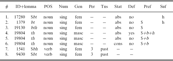
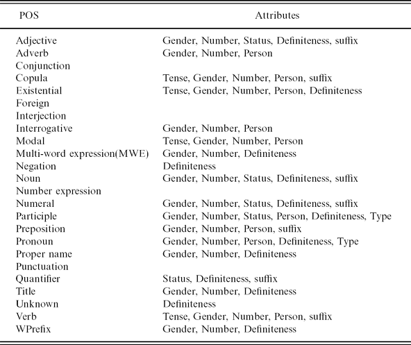
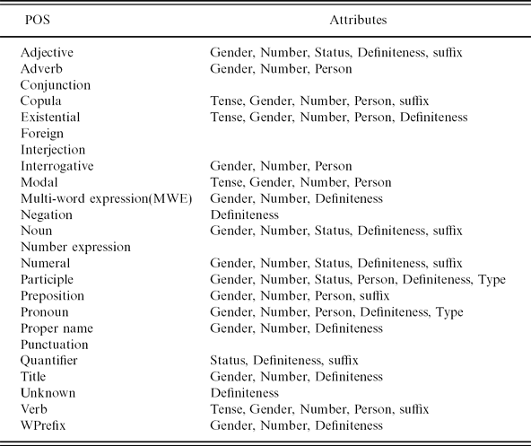
Our departure point in this work is the MILA morphological analyzer Itai and Wintner (Reference Itai and Wintner2008), a wide coverage, linguistically motivated morphological analyzer of Hebrew, which is based on a finite-state morphological grammar (Yona and Wintner, Reference Yona and Wintner2008) but is reimplemented in Java (Wintner, Reference Wintner2008). The output that the analyzer produces for the form $bth is illustrated in Table 1. In general, it includes the part-of-speech (POS) as well as the sub-category, where applicable, along with several POS-dependent features such as number, gender, tense, nominal state, definiteness etc. Table 2 shows the relevant attributes for each major POS category.
The analyses of the form $bth. Each analysis specifies a unique ID for the lemma, the lemma itself, its part-of-speech, number, gender, person, tense, nominal status, definiteness, prefixes and suffixes

Part-of-speech (POS) categories and their possible attributes
1.3 Hebrew morphological disambiguation
Morphological analyzers produce, for each word, all its valid analyses, independently of the context in which the word occurs. Morphological disambiguation is the task of ranking the grammatically valid analyses of each word, taking into account the context and producing the most likely analysis. This task is reminiscent of POS tagging, but is more challenging for languages with rich morphology (see Section 1.4).
The first stochastic approaches to Hebrew morphology could not rely on the existence of an annotated corpus. Hence, the primary task of such works was to approximate the morpho-lexical probability of each word in a given text (Levinger, Ornan and Itai 1995). Given a text T with n words w 1,…,wn, for each morphologically ambiguous word wi whose analyses are A 1,…,Ak, there is one analysis, Ar ∈ {A 1,…Ak}, which is the correct analysis in context. The morpho-lexical probability of an analysis Ai for some word w is the estimate of the conditional probability P(Ai|w) from a given corpus:
 \[
P(A_i\mid w)={\textit{\textup{Number of times }$A_i$ \textup{is the correct analysis of}
$w$}\over\textit{\textup{Number of occurrences of} $w$}}
\]
A similar approach is used by Carmel and Maarek (Reference Carmel and Maarek1999). To overcome the problem of data sparseness, this system makes decisions based on the frequencies of morphological patterns associated with the analyses of input words, rather than the analyses themselves. The patterns consist of parts of speech and other morphological information, but essentially not the lexeme. Here, too, contextual information is not taken into account, and the system only prunes relatively unlikely candidates independent of where they occur using some pre-defined threshold. For evaluation, a set of 16,000 words were manually annotated. Accuracy is defined as the number of words for which the output of the system includes the correct analysis. At a threshold of 0, accuracy is 98 percent (very unlikely analyses are filtered out always, so 100 percent cannot be achieved) and the proportion of words with a single analysis is 62 percent. At a threshold of 0.5, accuracy is 86 percent (74 percent for ambiguous words) and 100 percent of the words are assigned a single analysis.
The first work which uses stochastic contextual information for morphological disambiguation in Hebrew is Segal (Reference Segal1999): Texts are analyzed using the morphological analyzer of Segal (Reference Segal1997); then, each word in a text is assigned its most likely analysis, defined by probabilities computed from a small tagged corpus. In the next phase the system corrects its own decisions by using short context (one word to the left and one to the right of the target word). The corrections are also automatically learned from the tagged corpus (using transformation-based learning). In the last phase, the analysis is corrected by the results of a syntactic analysis of the sentence. The reported results are excellent: 96.2 percent accuracy. More reliable tests, however, reveal accuracy of 85.5 percent only (Lembersky Reference Lembersky2003: 85). Furthermore, the performance of the program is unacceptable (the reported running time on ‘two papers’ is thirty minutes).
The early works described above were all hampered by the lack of annotated corpora for Hebrew. More recently, however, such corpora have become available through a treebank project (Sima'san et al., Reference Sima'an, Itai, Winter, Altman and Nativ2001) and the Knowledge Center for Processing Hebrew (Itai and Wintner, Reference Itai and Wintner2008), facilitating the application of advanced machine-learning techniques to the problem of morphological disambiguation.
Bar-Haim, Sima'an and Winter (Reference Bar-Haim, Sima'an and Winter2005, Reference Bar-Haim, Sima'an and Winter2008) describe a segmenter and POS-tagger for Hebrew based on Hidden Markov Models (HMMs). This disambiguation model for segmentation and part-of-speech is based on word segments (morphemes) rather than words. Word segments are referred to as identifying the prefixes, the stem and suffixes of the word. This work starts out from a morphological analyzer and a very small morphologically annotated corpus. A model whose terminal symbols are word segments is shown to be advantageous over a word-level model for the task of POS tagging. Hence, a morpheme-level model is proposed, where words are first divided into separate morpheme segments: prefixes, stem and suffix. Then a proper POS tag is assigned to each of these morphemes. A way to extend the morpheme sequence back to a full analysis is also shown. The definiteness morpheme is treated as a possible feature of morpheme terminals, and the definiteness marker's POS tag is prefixed to the POS tag of the stem. This way data sparseness is reduced. However, this method lacks some word-level knowledge that is required for segmentation, and hence a part of information that is usually found in Hebrew morphological analyses is ignored. The internal morphological structure of stems is not analyzed, and the POS tag assigned to stems includes no information about their root, pattern, inflectional features and suffixes. The accuracy of this segmenter is reported for both tagging (a tagset of twenty-one POS tags is used) and for segmentation, and is 90.51 percent for the former and 96.74 percent for the latter.
Unfortunately, this tagger/segmenter is not enough for full morphological disambiguation. Some features produced by the analyzer are not used by the tagger, but are needed for full disambiguation. Consider, for example, the word $bth (Table 1): Analyses 5 and 6 differ only in status. Such words are ambiguous in a way that is not solved by the segmenter, since it cannot distinguish between different lexical IDs or the different values of the status attribute. Consequently, the version of the tagger that was made available to us resulted in a much lower accuracy on the full disambiguation task (only 75.73 percent).
Adler and Elhadad (Reference Adler and Elhadad2006) present an unsupervised stochastic model, where the only resource used is a morphological analyzer (see Section 1.5). A morpheme-based model must learn both segmentation and tagging in parallel in an unsupervised manner, since the output sequence used for the learning and searching process is uncertain. Reported results on a large-scale corpus (6 M words) with fully unsupervised learning are 92.32 percent for POS tagging and 88.5 percent for full morphological disambiguation. Due to various technical difficulties, including inconsistent corpus versions, we were unable to reproduce these results on our corpus. Furthermore, our work addresses certain subtle distinctions between different morphological analyses that Adler and Elhadad (Reference Adler and Elhadad2006) ignore; in other words, their system retains some ambiguity that we resolve. These include the subtype of proper names (we distinguish between names of persons, locations, organizations etc.); the subtype of pronouns (personal, demonstrative, reflexive etc.); the function of participles (which can function as nouns, adjectives or verbs); and distinguishing between two analyses that only differ in their lemma. On the other hand, Adler and Elhadad (Reference Adler and Elhadad2006) provide analyses for out-of-vocabulary tokens, which our task does not handle (Section 2.1).
A supervised approach to morphological disambiguation of Arabic is presented by Habash and Rambow (Reference Habash and Rambow2005). This work shows that the use of a morphological analyzer and learning classifiers for individual morphological features improve the results of both tokenizing and POS tagging for Arabic.Footnote 3 Habash and Rambow (Reference Habash and Rambow2005) developed a supervised morphological disambiguator, based on a training corpus of two sets of 120 K words, which combines several classifiers. Every morphological feature is predicted separately and then combined into a full disambiguation result. The accuracy of the disambiguator is 94.8–96.2 percent (depending on the test corpus). One thing to note, though, is the high accuracy they report for the baseline of each classifier (96.6–99.9 percent, depending on the classifier). The baseline of the whole disambiguating process is 87.3–92.1 percent (depending on the test corpus). Although Habash and Rambow (Reference Habash and Rambow2005) use a similar approach to the one presented in the present work, and the number of tags is similar to the number of tags in Hebrew, the differences between Hebrew and Arabic still induce significant differences in the results. Furthermore, our training corpus is far smaller than the ones available for Arabic.
1.4 The challenge of disambiguation
The most common and successful techniques for POS tagging in English use HMM (Marshall, Reference Marshall1983; Cutting et al., Reference Cutting, Kupiec, Pedersen and Sibun1992), Transformation-based learning (Brill, Reference Brill1995) or more sophisticated learning algorithms (Roth and Zelenko, Reference Roth and Zelenko1998). With a baseline of 90–91 percent accuracy, it is not very surprising that the best POS taggers for English achieve an accuracy of 96–97 percent (Manning and Schütze, Reference Manning and Schütze1999, Section 10). Crucially, the size of the tagset for English is very small: the Penn Treebank tagset has forty-five tags (including punctuation), and other proposed tagsets (e.g., the Brown Corpus one) are all smaller than one hundred tags.
Stochastic POS taggers for English take advantage of the high baseline and the relatively small tagset. They also benefit from the relatively fixed word order of English and from the fact that many of the frequent functional words (prepositions, determiners etc.) are unambiguous; such words can be used as anchors to disambiguate their neighbors. Morphological disambiguation of Hebrew is a much more complex endeavor due to the following factors:
Segmentation. A single token in Hebrew can actually be a sequence of more than one lexical item. Consider again the token $bth discussed above (Table 1). It can be segmented in the following ways, each inducing a completely different sequence of POS tags:
In practice, most tokens in a running Hebrew text have only one possible segmentation. In particular, the length of a prefix sequence is rarely greater than 1.
Large tagset. In contrast to the limited tagset of standard POS tagging approaches in English, the number of potential tags in a language such as Hebrew (where the POS, morphological features and prefix and suffix particles are considered) is huge. The morphological analyzer that we use in this work produces twenty-seven different parts of speech, some with subcategories: five values for the number feature (including disjunctions of values), three for gender, three for person, eight for tense and three for nominal status. Possessive pronominal suffixes can have eighteen different values, and prefix particle sequences can theoretically have hundreds of different forms, although in practice only a few dozens are witnessed in a standard corpus. Clearly, not all the combinations of these values are possible, and many values are extremely rare (e.g., the value ‘dual’ of the feature ‘number’). Still, the number of tags observed in large corpora is in the thousands. Thus, Adler (Reference Adler2007) determines the number of tags in the Hebrew corpus he used to be 3,600.
Ambiguity. Due to the rich morphology and the problems of the orthography, Hebrew is highly ambiguous. In a particular corpus of 40,000 word tokens, the average number of analyses per word token was found to be 2.1, while 55 percent of the tokens were ambiguous (Levinger et al. Reference Levinger, Ornan and Itai1995: 385). Our analyzer outputs on average approximately three analyses per word token, and 63 percent of the tokens are ambiguous. Excluding punctuation, the average number of analyses per token is 3.4, and some words have as many as thirty-seven analyses. Furthermore, in many cases two or more alternative analyses share the same part-of-speech, and in some cases two or more analyses are completely identical, except for their lexeme. This is the case of $bth (see Table 1), whose verb analysis is in fact ambiguous with respect to the lexeme (which can be the third person feminine singular past tense of ‘capture, take as captive’ or of ‘go on strike’), and whose noun analysis is ambiguous too (‘her sitting’ versus ‘her Saturday’). Such phenomena make morphological disambiguation of Hebrew, in some extreme cases, closer to the problem of word sense disambiguation than to standard POS tagging.
Anchors. Anchors, which are often function words, are almost always morphologically ambiguous in Hebrew. For example, the most frequent token in Hebrew is at which is almost always a preposition (the accusative marker), but sometimes a personal pronoun (second person feminine singular) and, very rarely, a noun (‘spade’). Similarly, the frequent genitive preposition $l ‘of’, in some of its inflections, is highly ambiguous. Many of the function words which help boost the performance of English POS tagging are actually prefix particles which add to the ambiguity in Hebrew (e.g., the definite article h ‘the’ or the coordinating conjunction w ‘and’).
Word order. Word order in Hebrew is relatively free, and in any case much freer than in English.
1.5 Direct classification
While the number of possible analyses is potentially huge, several constraints hold among the values of different components of the analysis. For example, the tense feature is only relevant if the POS is verb, whereas definiteness is relevant only for nominals (nouns, adjectives, numerals and pronouns). As another example, the number of prefix particle sequences is theoretically large, but in practice no more than three or four prefixes are observed, with very strict (syntactically motivated) constraints on their order. Therefore, it may be possible to define a relatively small number of complex POS tags which uniquely cover the set of valid analyses.
Such a strategy is proposed by Adler and Elhadad (Reference Adler and Elhadad2006); it is based on the following two observations: first, a valid sequence of prefix particles in Hebrew can be at most of length 6 (characters),Footnote 4 and when its length is known, its segmentation is uniquely determined; second, if it is known that the word has a pronominal suffix, then this suffix can almost always be uniquely determined from the surface form of the word. Thus, a POS tag for Hebrew should consist of three components: an indication of the number of characters (0 to 6), which comprise the prefix sequence; a tag for the lexeme; and an indication of whether or not a pronominal suffix is present. The tag of the lexeme must capture the main and secondary part-of-speech, and a collection of features such as number, gender, person, tense, status etc. As an example of this strategy, consider again the case of $bth (see Table 1), whose analyses can be tagged as follows:
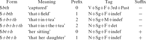
This encoding can then be used with standard POS tagging techniques to uniquely disambiguate a morphologically analyzed corpus. This work was further extended by Adler et al. (Reference Adler, Goldberg, Gabay and Elhadad2008a), who focus on obtaining the correct analysis for out-of-vocabulary items, a task that we do not address in the present work. However, the direct classification approach has two shortcomings. First, the number of tags remains very high: with seven possible values for the location of the prefix sequence (0–6), approximately fifty tags for the lexeme and two values for the suffix, the tag set has 700 members. For languages with more complex morphology than Hebrew, in particular agglutinative languages, this number can reach thousands of categories, thereby reducing the potential of standard classification methods to perform accurately. Second, this encoding does not suffice to uniquely disambiguate the corpus in the face of analyses which differ only in the lexeme, or in the subtype of POS categories, as we have seen above (Section 1.3). We therefore opt for the more complex, yet more promising technique of combining classifiers.
1.6 Classifier combination
Making natural language decisions often involves assigning values to sets of variables where complex and expressive dependencies can influence, or even dictate, what assignments are possible. This is clearly the case for the problem of morphological disambiguation: one can learn relatively accurate classifiers for various components of the analysis, such as the main POS, or the correct segmentation of the word form, or whether or not the form is definite. Obviously, such decisions are highly inter-dependent, and in particular, the combination of the predictions of the classifiers must respect the constraints imposed by the morphological analyzer, namely that the resulting analysis is indeed one of the analyses produced by the analyzer. As an example, consider again the form $bth. A POS classifier can predict that the main POS tag is VBD, whereas a segmentation classifier can predict that the initial $ is a prefix; the two predictions are inconsistent, given the valid analyses produced by the analyzer. Of course, if the classifiers not only predict a single candidate but rather rank all possible candidates, a more sophisticated method of combining their results can yield predictions which are consistent with the constraints imposed by the analyzer.
Efficient solutions have been given to problems of this kind under some restrictions. One class of solutions decouples the process of learning estimators to variables' values from the inference process that is applied later, to derive a global assignment to the set of variables of interest. A second class of solutions incorporates the dependencies among the variables into the learning process, and directly induces estimators that yield a (good) global assignment. HMMs, conditional models (McCallum, Freitag and Pereira Reference McCallum, Freitag and Pereira2000; Punyakanok and Roth Reference Punyakanok and Roth2001) and a large number of dynamic programming schemes used in the context of sequential predictions fall into the first category. Conditional Random Fields (Lafferty, McCallum and Pereira Reference Lafferty, McCallum and Pereira2001) and other discriminative learning methods with Markov assumptions are in the second category.
In this work we use a different solution. We decouple the multi-class classification task into several simple processes and then combine the results under the constraints imposed by a linguistically informed morphological analyzer. This approach was shown to be successful for identifying the roots of Semitic words (Daya, Roth and Wintner 2004, 2008) and for the Arabic morphological disambiguation (Habash and Rambow, Reference Habash and Rambow2005). Combining machine learning with limited linguistic knowledge was shown to produce state-of-the-art results on difficult morphological tasks.
2 Methodology
2.1 Task
Our task in this work is to induce a consistent ranking on the analyses produced by the morphological analyzer. Similar to Similar to Hajič (Reference Hajič2000), Habash and Rambow (Reference Habash and Rambow2005) and Daya et al. (Reference Daya, Roth and Wintner2004, Reference Daya, Roth and Wintner2008), we approach the problem of morphological disambiguation as a complex classification task. We train a classifier for each of the attributes that can contribute to the disambiguation of the analyses produced by the analyzer (e.g., POS, tense, state). Each classifier predicts a small set of possible values and hence can be highly accurate. In particular, the basic classifiers do not suffer from problems of data sparseness. Of course, each simple classifier cannot fully disambiguate the output of the analyzer, but it does induce a ranking on the analyses. Then, we combine the outcomes of the simple classifiers to produce a consistent ranking which induces a linear order on the analyses.
Note that each classifier ranks only the options that are valid for the target word. If the analyses of a given word specify, for example, only two values for parts of speech: noun and verb, the POS classifier only ranks those two for this word and gives a 0 score to the other POS values. In this way, the classifiers induce a ranking on the analyses themselves. For example, ranking the two POS values of the analyses of Table 1 directly induces a ranking of those analyses, where analyses whose main part of speech is noun (analyses 1–6) are ranked the same, as are analyses with main POS verb (7–8).
Note also that the task does not involve induction of tags on all words in a text; if a word is unknown to the morphological analyzer, it is up to the analyzer to suggest an analysis for it (its current policy is to suggest proper noun analyses, by stripping potential prefixes from the word form). Our task is only to rank the output of the analyzer.
2.2 Corpora
For training and evaluation, we manually annotated a corpus of 3,989 sentences (72,062 tokens) taken from the daily newspaper HaAretz. The annotation consists of selecting the correct analysis produced by the analyzer, or an indication that no such analysis exists. The corpus was annotated by two annotators, and a trained lexicographer consolidated the two annotations and resolved any inconsistencies. Most of the corpus (3,325 sentences; 59,870 tokens) is used for training and the remaining part (664 sentences; 12,192 tokens, of which 2,734 do not occur in the training corpus) is for development.
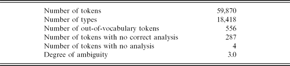
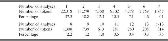
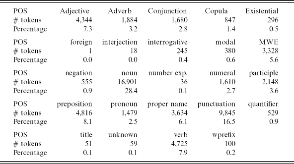
Tokens for which the lexicographers determined that the correct analysis is not produced by the analyzer are disregarded during the experiments; such tokens reflect limitations of the analyzer, but do not affect the task of disambiguation. The corpus also includes very few tokens for which no analysis was produced, again reflecting some problem of the analyzer. Finally, when the analyzer encounters an unknown word, it typically assigns it a proper name analysis, but indicates the fact that no lexical entry exists for this token; we refer to such tokens at out-of-vocabulary (OOV). Some statistics on the training corpus are given in Tables 3–5.
Statistics of training corpus
Histogram of number of analyses in the training corpus
Distribution of parts of speech in the training corpus
For testing, we also manually annotated a small corpus of one hundred sentences (1,537 tokens, of which 395 do not occur in the training corpus) from the same newspaper (but a very different period). Finally, we also use a large (32 M tokens) unannotated corpus, this time of various sources (Itai and Wintner, Reference Itai and Wintner2008), to obtain word- and analysis-frequency statistics (see Section 3.4).Footnote 5
2.3 Classification Method
In all the experiments described in this paper we use SNoW (Roth, Reference Roth1998) as the learning environment, with winnow as the update rule. SNoW is a multi-class classifier that is specifically tailored for learning in domains in which the potential number of information sources (features) taking part in decisions is very large, of which NLP is a principal example. It works by learning a sparse network of linear functions over a pre-defined or incrementally learned feature space. SNoW has been already used successfully as the learning vehicle in a large collection of natural language related tasks, including POS tagging, shallow parsing, information extraction tasks etc., and compared favorably with other classifiers (Roth, Reference Roth1998; Punyakanok and Roth, Reference Punyakanok and Roth2001; Florian, Reference Florian2002). Typically, SNoW is used as a classifier, and predicts using a winner-take-all mechanism over the activation values of the target classes. However, in addition to the prediction, it provides a reliable confidence level in the prediction, which enables its use in an inference algorithm that combines predictors to produce a coherent inference.
2.4 Baseline
For evaluation we consider only the words that have at least one correct analysis in the annotated corpus. Our measure of evaluation is accuracy, defined as the ratio of the number of words classified correctly to the total number of words in the test corpus that have a correct analysis. First, we report the performance of simple classifiers tested on a development subset with which we tune several parameters. We then report the results of classifier combination, obtained by training on the entire training corpus and testing on the development and the test corpora. In addition, we perform ten-fold cross-validation runs on the entire training corpus and report the average of ten runs.
The baseline tag of a token w is an ID of the most prominent analysis of all the occurrences of w in the training corpus. This is the analysis that was annotated as the correct one for this token more times than any other analysis. Table 6 illustrates this idea: Suppose a token w has three analyses, and suppose that w occurs ten times in the training corpus. The first analysis was annotated as the correct one in three instances, the second analysis in four and the last analysis in three. Then the baseline tag of w is the ID of the second analysis. The baseline tag of a token also induces a baseline tag for every feature of this token, like part-of-speech, gender, person etc. In the example of Table 6, the baseline POS of w is verb, the baseline gender is masculine and the baseline person is second.
An example of the baseline tag

If w does not occur in the training corpus, we back off and select the baseline tag of each feature of w from the corpus independent of the word w. That is, if a noun is more prominent in the corpus than a verb, then a noun will be chosen as the baseline tag of the POS feature of w. It is more difficult to induce the baseline tag (i.e., the most prominent analysis ID) of such unseen tokens. We rank each analysis based on a number of its features that have the most prominent values. The analysis that receives the highest score is then selected as the baseline tag of w. For example, suppose that the most prominent value of part of speech in the corpus is noun, the gender is feminine and the person is n/a (not applicable). In this case, the first analysis in the example of Table 6 scores one point (for gender), the second analysis scores zero point and the third one scores three points (POS, gender and person). Consequently, in this case the third analysis is chosen as the baseline tag of w. We now define these notions formally.
Let w be a word token (e.g., $bth), and let #w be the number of occurrences of w in the training corpus. Assume that the morphological analyzer produces k analyses for (each occurrence of) w (e.g., Table 1 shows k = 8 for w = $bth). Let fi be a feature of the analysis, 1 ≤ i ≤ F. Let fij, where 1 ≤ j ≤ k, be the value assigned by the jth analysis to feature fi. Again using the example of Table 1, f 1 is part of speech and while f 13 is noun, f 17 is verb.
Let Ajw be the number of occurrences of w for which the jth analysis is annotated as the correct one. For example, if w = $bth, then A $bth3 is the number of occurrences of $bth in the corpus in which the third analysis is annotated as the correct one. For each feature fi, 1 ≤ i ≤ F, let Bij be the number of times fij is the correct value of fi in the training corpus. Crucially, Bij is independent of w. For example, if f 1 is the feature POS, then B17 is the number of tokens in the corpus for which the value of the POS feature is verb.
For predicting the value of some feature fi, the baseline tag of some token w is
 \[
\hat{t}(f_i,w)=\left\{\begin {array}{ll}
f_i^{\hat{j\;}}\!\mbox{, where } \hat{j}=argmax_{j}A^{j}_{w}&\mbox{if $\#w > 0$}\\[2pt]
f_i^{\hat{j\;}}\!\mbox{, where } \hat{j}=argmax_{j}B^{j}_{i}&\mbox{if $\#w = 0$}
\end{array}\right.
\]
As for the analysis ranking task, again if w occurs in the training corpus, the baseline analysis is the most frequent analysis assigned to w. If w does not occur in the corpus, however, we define a voting mechanism among all the features that are involved in the analysis of w. Let Cjw be the score function of analysis j of some token w, given by
 \[
\label{eq:score_function}
C^j_w = \sum_{1\le i\le F}{\Lambda(f_i^j)}
,\mbox{ where }
\Lambda(f_i^j)=\left\{\begin {array}{ll}
1 & \mbox{if $\hat{t}(f_i,w) = f_i^j$}\\
0 & \mbox{otherwise}
\end{array}\right.
\]
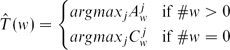 \[
\hat{T}(w)=\left\{\begin {array}{ll}
argmax_{j}A^{j}_{w}&\mbox{if $\#w > 0$}\\[2pt]
argmax_{j}C^{j}_{w}&\mbox{if $\#w = 0$}
\end{array}\right.
\]
3 Disambiguation by classification
We decouple the task of morphological disambiguation by defining several basic classifiers. The predictions of the classifiers are then combined to yield a consistent prediction.
3.1 Simple classifiers
The simple classifiers are all built in the same way. These are trained on feature vectors that are generated from the annotated output of the morphological analyzer. We define several classifiers for the attributes of the morphological analyses. Note that some attributes do not apply for all the analyses (see Table 2). For example, the attribute ‘tense’ is inapplicable for an analysis whose main part of speech is noun. We therefore add a value of ‘irrelevant’ for inapplicable attributes. Also, in some cases the corpus does not have a value for some feature for which such a value is necessary. In such cases, the corpus usually lists the value as unspecified; we account for these values as well. We describe each of the classifiers below.
Part-of-speech (POS). The (POS) classifier predicts the main part of speech of the word. The possible values of this attribute are ‘adjective’, ‘adverb’, ‘conjunction’, ‘copula’, ‘existential’, ‘foreign’, ‘interjection’, ‘interrogative’, ‘modal’, ‘MWE’, ‘negation’, ‘noun’, ‘number expression’, ‘numeral’, ‘participle’, ‘preposition’, ‘pronoun’, ‘proper name’, ‘punctuation’, ‘quantifier’, ‘title’, ‘unknown’, ‘verb’ and ‘wprefix’.
Segmentation. The segmentation classifier predicts the index of the beginning of the base. This classifier ranks seven options [0–6], where 6 is the length of the longest possible prefix sequence.
Gender. The gender classifier ranks five values: ‘masculine’, ‘feminine’, ‘masculine and feminine’, ‘unspecified’ and ‘irrelevant’.
Number. The number classifier ranks seven values: ‘singular’, ‘plural’, ‘dual’, ‘singular and plural’, ‘dual and plural’, ‘unspecified’ and ‘irrelevant’.
Person. The person classifier ranks six values: ‘first’, ‘second’, ‘third’, ‘any’, ‘unspecified’ and ‘irrelevant’.
Has properties. This is a binary classifier distinguishing between categories that are atomic (e.g., conjunction, interjection, interrogative, negation, punctuation and quantifier) and categories whose words have attributes (e.g., noun, adjective, adverb, auxiliary verb, particle, preposition, pronoun, proper name and verb).
Tense. The tense classifier ranks nine values: ‘past’, ‘present’, ‘beinoni’, ‘future’, ‘imperative’, ‘infinitive’, ‘bare infinitive’, ‘unspecified’ and ‘irrelevant’.Footnote 6
Definite article. The definiteness classifier ranks four values: ‘definite’, ‘indefinite’, ‘unspecified’ and ‘irrelevant’. It identifies both implicit and explicit forms of definiteness.
Status. The status classifier ranks five values: ‘absolute’, ‘construct’, ‘absolute and construct’, ‘unspecified’ and ‘irrelevant’.
Pronoun type. The pronoun type classifier ranks eight values, reflecting the different sub-categories of Hebrew pronouns: ‘personal’, ‘demonstrative’, ‘relativizer’, ‘impersonal’, ‘reflexive’, ‘interrogative’, ‘unspecified’ and ‘irrelevant’.
Participle type. The participle classifier ranks seven values, reflecting the function of the participle in the sentence: ‘noun’, ‘noun or adjective’, ‘noun or verb’, ‘noun or adjective or verb’, ‘adjective’, ‘verb’ and ‘irrelevant’.
These classifiers are (almost) sufficient for full disambiguation, see Section 3.4.
3.2 Training the simple classifiers
3.2.1 Feature set
Each word in the training corpus induces features that are generated for itself and its immediate neighbors (the ‘window’). These features are generated from the output of the morphological analyzer. For each word in the window, we generate the following features:
• The main part-of-speech (twenty-five options)
• Number (seven options)
• Gender (five options)
• Person (six options)
• Tense (nine options)
• Status (five options)
• Definite article (four options)
• Relevant features. In order to emphasize the value of ‘irrelevant’ in some of the attributes, we created an additional feature for those attributes that are not applicable to all the parts of speech (see Table 2). These features are binary features whose values are ‘relevant’ and ‘irrelevant’. For example, tense is not relevant for an analysis whose part of speech is noun. The features are ‘is the number relevant’ (this is the disjunction of all the values of ‘Number’ except ‘irrelevant’), ‘is the gender relevant’, ‘is the person relevant’, ‘is the tense relevant’, ‘is the status relevant’ and ‘is the definite article relevant’.
• All the prefixes (twelve options). Each of the possible prefixes of Hebrew (such as ‘m’, ‘$’, ‘m$’ etc.) is a feature; this feature indicates if an analysis has one of those prefixes.
• Number–gender–person combination of the suffix. As described in Section 1.1, nominals take pronominal suffixes which inflect for number, gender and person. This inflection is combined into a single value (there can be 210 options; 5 Gender × 7 Number × 6 Person).
• Does the word have a suffix? (two options)
• Complex POS (a feature that combines the part of speech of the prefix, base and suffix) (200 options). This feature represents the full POS of a surface form, and is created from the cartesian product of twenty-five values of POS, four values of the prefix POS (‘conjunction’, ‘preposition’, ‘determiner’ and ‘relativizer/subordinator’) and an indication of whether the word has a suffix.
• The surface form of the word (as many values as the size, in types, of the training corpus).
• The lemma of the base (approximately 21,000 values, the size of our lexicon). To reduce data sparseness, we consider not only the surface form of the word but also its lemma.
3.2.2 Determining the window size
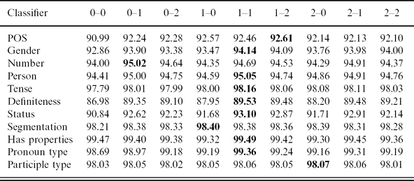
Each of the supervised classifiers can be configured in several ways. First we need to determine the size of the training and testing window. We experimented with several window sizes, up to two words before and after the current word. Table 7 depicts the best window size for each classifier. (We used the development set in these experiments.)
Accuracy of all basic classifiers, varying window sizes
3.2.3 Determining feature values in sequential prediction
Our task is sequential in nature: Determining the part of speech of the current word obviously depends on the part of speech of its immediate neighbors. This information is known during training, but not at actual testing time. Therefore, one must decide how to handle this uncertainty.
One question is whether or not to use the correct analysis of the target and its adjacent words when generating feature vectors. The correct analysis is available during training, but not during testing. Obviously, the correct analysis can improve the accuracy of the prediction; but using it for training creates a discrepancy between the training process and the way features are generated for testing. In order to keep training and testing feature vectors consistent, we therefore use instead the most prominent feature values, determined by the same criteria that are used for baseline computation (see Section 2.4) in both testing and training. Experimenting with different approaches yielded worse results.
Another question involves the proper treatment of words that are not present in the training material (unseen items). For such words, which are again only present at test time, the only possible solution is to generate feature vectors that are independent of the word itself. For example, when a value for the feature POS is generated for some unseen word w, this value is determined to be the most frequent part-of-speech in the training corpus, independent of w. Referring back to Section 2.4, the question is whether to use Awj or Cwj for computing  (w). Again, this entails a discrepancy between the way features are generated for training and testing. To overcome this problem, we experiment with three ways to generate features at training:
(1) Generate features based on the actual words in the text (since no unseen items exist during training).
(2) Generate features based on the actual words for a randomly determined portion of the training corpus, and treat all other tokens as unseen. We chose 25 percent as the portion of the text treated as unseen, reflecting the ratio of unseen items in our corpus.
(3) Generate features as if all words in the training and testing corpus are unseen.
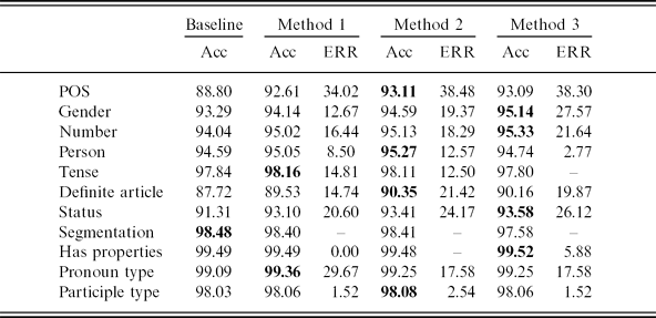
The results of all these experiments are shown in Table 8. We report the accuracy of each classifier and the reduction in error rate (ERR), compared to the baseline, which is defined as in Section 2.4.
Accuracy and error-rate reduction of simple classifiers, compared with the baseline, reflecting three methods for feature generation during training
Clearly, most classifiers perform much better than the baseline. Specifically, on the important task of POS tagging we demonstrate decent accuracy of 93.1 percent and reduction of almost 40 percent of the errors compared with the baseline. High gains are clearly evident for other classifiers as well, the only exception being the segmentation classifier, for which the baseline performs slightly better. We do not have any explanation for this phenomenon.
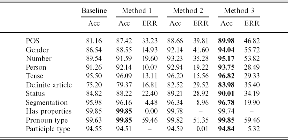
Interestingly, for six out of eleven classifiers, the third method outperforms the first one even though it uses less accurate information during both training and testing. This effect is enhanced when only unseen items are considered. Table 9 displays exactly the same evaluation, constrained only to unseen items. The third method is the best for ten out of eleven classifiers.
The same evaluation as in Table 8, limited to unseen items only
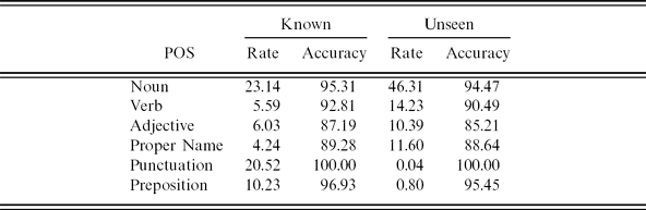
These results also demonstrate quite clearly that the classifiers perform much worse on unseen words than on seen ones. This is not surprising; it stems from the fact that unseen words are much less common in the text than known words, and the distribution of their POS classes is quite different from that of known words. For example, unseen words rarely belong to closed POS classes, like punctuation or preposition. On the other hand, words in closed classes comprise more than 30 percent of the text and are usually not ambiguous. Table 10 depicts the distribution of major POS classes among seen and unseen tokens in the development corpus, exhibiting significant differences. In particular, almost half of the unseen tokens are nouns, and 14 percent of them are verbs, compared to one-quarter and 5.54 percent, respectively, of the known tokens. On the other hand, more than 20 percent of the known tokens, but none of the unseen ones, are punctuation.
Part-of-speech distribution in the development corpus and the accuracy of the POS classifier: known versus unseen tokens
We also report in Table 10 the performance of the POS classifier on specific POS classes, for known words and unseen ones. The classifier performs much better on the closed POS classes, like punctuation and prepositions, than on open classes, in particular adjectives and proper names. Since the closed POS classes are much more common among known words, this explains the gap between known and unseen words in the overall performance of the POS classifier.
Based on these observations, we conclude that the third training scenario performs best, especially on the more difficult cases. Also, it does not rely on token-specific information, such as the most prominent analysis, and therefore it is more robust. This is then the method we adopt in this work.
3.3 Combination of classifiers
Classifier combination is based on the fact that linguistic knowledge is incorporated into the analyzer. Each analysis is created using a set of morphological rules, and thus the attributes of a specific analysis satisfy those morphological constraints. Each classifier predicts a single morphological feature, which induces a rank of the entire list of analyses.
To combine the predictions of the simple classifiers, we accumulate the scores of all the classifiers. We experiment with three types of combinations: naïve, linear and hierarchical.
Naïve combination. We use the confidence level of each SNoW classifier as the score. We accumulate the scores of all the classifiers, yielding a single score per analysis, thereby inducing a rank on the list of analyses.
Linear combination. We treat the problem of combining the outcomes of the classifiers as a linear regression problem. We define the error as the ratio of wrongly disambiguated tokens to the size of the corpus. Each classifier is a variable in a linear function. The coefficients are induced in a procedure called Powell's search (Powell, Reference Powell1964), which is a common method for finding the minimum of a function of several variables without computing derivatives. We use the development corpus to optimize weights.
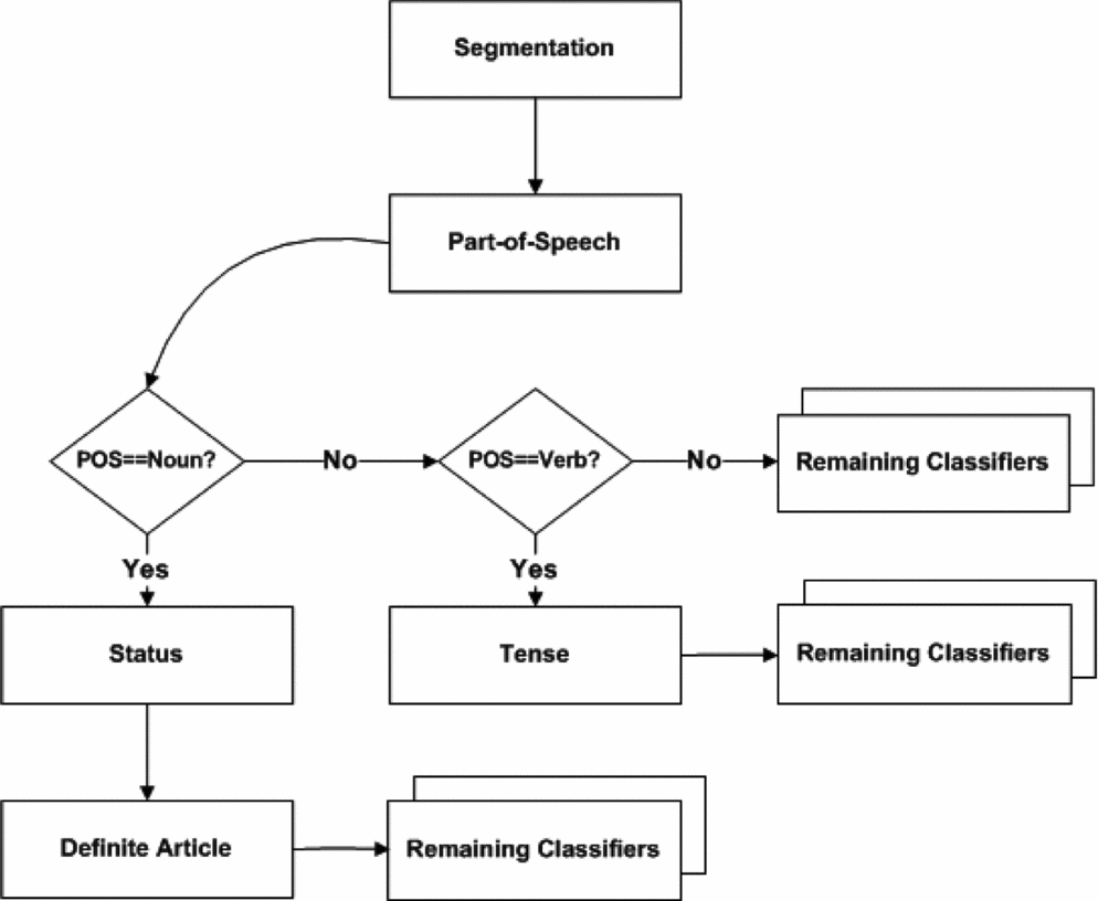
Hierarchical combination. The classifiers are applied one-by-one in a predefined order that is based on linguistic knowledge. Each step reduces the level of remaining ambiguity until a token is fully disambiguated or there are no more classifiers. Figure 1 shows the order in which the classifiers are applied.
Hierarchical combination.
3.4 Backing off to unsupervised classification
None of the combination strategies discussed above can guarantee a single, unique top-ranked analysis. This is because in some cases two or more analyses with identical morphological features differ only in their lexical ID. Distinguishing between such analyses requires word sense disambiguation rather than morphological disambiguation (Section 1.4). Solving this problem is beyond the scope of this work, and therefore we use a simplistic approach to disambiguate such analyses. We train an additional unsupervised classifier that chooses the most frequent lexical item. The frequencies are computed from a large morphologically analyzed (but not annotated or disambiguated) corpus (Section 2); see also Levinger et al. (Reference Levinger, Ornan and Itai1995) and Carmel and Maarek (Reference Carmel and Maarek1999).
Given a word with two analyses that only differ in their lexical ID, such as analyses 7 and 8 in Table 1, we break the tie by preferring the analysis reflecting the lexical ID that is more frequent in the unannotated (larger) corpus. The motivation for this step is the observation that such forms may have different inflectional paradigms, so that other inflected forms of the same lexical ID can be more or less frequent in the unannotated corpus. Note that even this does not guarantee full disambiguation: some (different!) base forms have completely identical inflectional paradigms, and hence the unannotated corpus will have exactly as many occurrences as one of the analyses of the other.
3.5 Results
Tables 11 and 12 depict the accuracy of our disambiguation module with and without the unsupervised backoff module described in Section 3.4. As described above we report ten-fold cross-validation results for the training set (59,363 tokens), as well as the results of training on the entire training set and testing on the development (12,189) and test (1,537 tokens) sets. In all experiments we use the third training scenario (Section 3.2). We also provide the baselines defined in Section 2.4.
Results: accuracy of full disambiguation without backoff
Results: accuracy of full disambiguation with backoff
The results show that the naïve combination outperforms other combinations on the ten-fold cross-validation task and on the test set. In this scenario, the overall accuracy of full morphological disambiguation is 84.15 percent under ten-fold cross-validation evaluation, reflecting a reduction of approximately one quarter of the errors compared with the baseline. The accuracy on the (out-of-domain) test set is only slightly lower, i.e., 82.63 percent. The contribution of the unsupervised backoff module is an additional 1.5 to 1.9 percent points.
A statistical significance analysis, performed on the results of the ten-fold cross-validation experiments, shows that all combinations are statistically better than the baseline (p < 0.001). Both the naïve (p < 0.001) and the linear (p < 0.01) combinations are statistically better than the hierarchical combination; and finally, the difference between the naïve and the linear combinations is not statistically significant.
To better appreciate the contribution of our method, we conducted yet another evaluation, in which we ignored some subtle distinctions that previous works (in particular, Adler and Elhadad Reference Adler and Elhadad2006) do not consider as significant. In other words, we view as ‘correct’ analyses that only differ from the human-annotated analysis in the sub-category of the main POS (for pronouns, proper names, participles etc.) or in the lexical ID. In such a scenario, the accuracy of the disambiguation module is 86.14 percent on the test set, 88.58 percent on the development set and 88.00 percent under ten-fold cross-validation runs. These figures compare favorably with the best reported results on this task.
Finally, to emphasize the contribution of classifier combination, we also evaluated the accuracy of the disambiguation module in predicting only the major POS category of each word. This is obtained simply by projecting the correct analysis onto the POS coordinate. Whereas the simple POS classifier was correct in 91.54 percent of the cases on the test set (93.09 percent on the development set), the disambiguator yields the correct POS in 92.19 percent of the words in the test set (93.89 percent of the development set, 93.17 percent under ten-fold cross-validation evaluation), a small but significant improvement, reflecting around 10 percent reduction in error rate. Other simple classifiers, predicting other features of the analysis, improve similarly in this way.
4 Error analysis
In this section we analyze the most frequent errors resulting from the disambiguation of the test set by the best performing system. Out of the 1,537 tokens, the system incorrectly disambiguated 239 tokens and another twenty-eight tokens remain ambiguous. We distinguish between incorrect and partially disambiguated tokens and provide a list of the most common errors in both cases.
4.1 Incorrectly disambiguated tokens
Construct. In many cases our system fails to correctly identify whether the word is in the absolute or the construct state. This problem is responsible for 14.6 percent of all errors. Overall, the system fails in 1.8 percent of the cases with this particular ambiguity.
Hidden definite article. One of the peculiarities of the Hebrew orthographic system is that the definite article ‘h’ is omitted, then it directly follows one of the prepositions ‘b’, ‘l’, ‘k’. In many such cases the system mistakenly tags the words as indefinite. This issue is responsible for 12.9 percent of all errors. The system fails in 3.5 percent of relevant cases.
Participles. Participles are often mistagged as nouns, adjectives or verbs. In few cases, words that were tagged as participles are in fact verbs in the past tense, nouns or adjectives. Participle-related errors are responsible for 10 percent of all errors, and 3.1 percent of the cases involving participle-related ambiguity are tagged wrongly.
Proper name. The Hebrew orthography does not capitalize proper names. In addition, many Hebrew proper names are derived from common nouns. Consequently, distinguishing proper names from nouns is challenging. The system makes quite a few mistakes (8.8 percent of all errors), mistagging nouns as proper names and the other way around, resulting in 5.2 percent of all cases with such ambiguity.
Noun versus verb. In some cases nouns can be mistakenly identified as verbs and the other way around. This is especially true for nominalizations of verbs. This issue is responsible for 5.9 percent of all errors. Less than 1 percent of the cases with this ambiguity are mistagged by the system.
Noun versus adjective. Another similar issue is the orthographic similarity between nouns and adjectives. For example, the word $kv can mean either ‘silence’ (noun) or ‘silent/pacific’ (adjective). This ambiguity is responsible for 5.4 percent of all errors. Only 0.5 percent of the relevant tokens are mistagged.
Wrong lexical item. The system resolves word sense ambiguity using an unsupervised classifier based on the frequency of lexical items in an analyzed, but not annotated, corpus. The wrong choices of this classifier are responsible for 5 percent of all errors and 20 percent of the relevant cases.
Participle subtype. Participles have three possible subtypes: verb, noun or adjective. In some cases (4.2 percent of all errors) the system fails to make the correct choice. This happens in 1.3 percent of the relevant cases.
Proper name subtype. Proper names are subcategorized to persons, locations and organizations. For example, the proper name lwndwn ‘London’ can refer to a person or to the city. The errors in proper name subtype comprise 2.9 percent of all errors (less than 1 percent of the cases with proper name subtype ambiguity).
Pronoun versus copula. Personal pronouns and copulas have some common forms in Hebrew, which have to be disambiguated. This issue is responsible for 2.9 percent of all errors or 7.3 percent of the cases with such ambiguity.
Multi-word expressions (MWE). In some cases the system fails to identify that a word belongs to a MWE and tags it as if it was a stand-alone word. This issue is responsible for 2.9 percent of all errors; 1.4 percent of MWEs are mistagged by the system.
4.2 Partially disambiguated tokens
Quantifier subtype. Our disambiguation module does not distinguish between partitive and determinizing quantifiers. This issue is responsible for 35.7 percent of all partially disambiguated tokens. The easiest way to overcome this problem is to construct an additional classifier for determining the subtype of a quantifier.
Lexical item. In some cases even the unsupervised classifier cannot make a distinction between different senses of a word. For example, $ibh can mean either ‘return’ or ‘old age’. Both are nouns, and both occur in exactly the same inflected forms, and hence cannot be distinguished by the unsupervised classifier. This issue explains 21.4 percent of all partially disambiguated tokens. Note that this is really an issue of word sense, rather than morphological, disambiguation.
Proper name subtype. Misclassification of the category of proper names is responsible for 17.9 percent of partial disambiguation. Again, a dedicated classifier could alleviate some of the problem here.
Suffix. In some cases the system fails to tell whether or not a word (typically, ending with i) has a pronominal suffix. For example, the word axri can mean either ‘after’ or ‘after me’ depending on whether it has a pronominal suffix or not. This issue is responsible for 14.3 percent of all partially disambiguated tokens.
5 Conclusions
Morphological disambiguation of Hebrew is a hard task. It involves, in theory, thousands of possible tags, although in practice only a few hundreds are witnessed in a standard corpus. As shown by Habash and Rambow (Reference Habash and Rambow2005), decoupling this task into several simple tasks improves the accuracy of morphological disambiguation for Arabic. We have shown here that using the same techniques for Hebrew improves accuracy over the baseline. Our best result, 84.15 percent accuracy, was obtained using simple supervised classifiers, for each individual morphological feature, backing off to an unsupervised classifier to reduce the remaining ambiguity.
We believe that these results can be further improved in various ways. The use of supervised machine-learning methods requires large annotated corpora for training. In this work we used a very small corpus, of a little less than 60,000 word tokens. Increasing the size of the training corpus can improve the accuracy of the basic classifiers, and hence of the full disambiguation process. As an indication that more training material is likely to improve the accuracy, we depict in Figure 2 a plot of the accuracy of the full disambiguation task as a function of the size of the training corpus. As the learning curve clearly shows, the improvement is nearly linear, and we thus have good reasons to believe that convergence of the accuracy is still faraway.
Learning curve.
We also expect that fine-tuning of the classifiers, and in parallel, fine-tuning of SNoW, can also improve the accuracy of the basic classifiers. Another potential direction for future research would be to investigate more sophisticated methods for combining the outcomes of various classifiers. While our results demonstrate that the hierarchical combination does not improve the accuracy, one could possibly rely on classifiers with higher confidence first, and use their predictions to reduce the ambiguity and only then use less confident classifiers.
Perhaps the most promising research direction, however, is in combining morphological disambiguation with parsing. In languages with rich morphology, such as Hebrew, these two tasks are closely related and highly intertwined; a joint solution is likely to improve the accuracy of both tasks. Several preliminary works have recently explored this direction (Tsarfaty Reference Tsarfaty2006; Cohen and Smith Reference Cohen and Smith2007; Goldberg and Tsarfaty Reference Goldberg and Tsarfaty2008; Lee, Naradowsky and Smith Reference Lee, Naradowsky and Smith2011); further research is still needed in order to obtain the best possible results.
Acknowledgments
We are extremely grateful to Dan Roth for his support and advice; to Inbar Tubi, Yuval Pinter and Gily Chen for corpus annotation; and to Dalia Bojan, Gassan Tabajah, Yossi Jacob and Alon Itai for the implementation and support of the corpora and morphological analyzer. This research was supported by The Israel Science Foundation (Grants No. 137/06).