1. Introduction
Autonomous mobile robots, such as automatic guided vehicles, are receiving much attention from researchers due to their significant enhancement of task execution efficiency in applications within the military [Reference Zhai, Zhang, Xu, Yuan, Zhou and Wu1], agriculture [Reference Lin, Xu, Zhou and Chen2], and other fields [Reference Hassan, Eberhardt, Malorodov and Jäger3–Reference Ramos, Pinto and Haddad7], of which a critical technology is the pose estimation technology. Pose estimation aims to provide precise front-end information for the subsequent control and decision task of robots by accurately estimating the pose of itself or the object, where some typical applications include precise navigation in autonomous driving [Reference Ding, Pei, Yang and Chen8, Reference Zeng, Zhong, Wang, Fan and Zhang9] and the effective object grasping for robotic arms [Reference Liu, Shi, Zhou, Wang, Zhang and Dong10, Reference Zhou, Luo and Wang11]. Pose estimation technology has always been a current research hotspot in the field of robotics.
Up to now, many algorithms that depend on various sensors (e.g., inertial sensors, GPS, and radar) have been proposed for pose estimation problems [Reference Liu and Guo12–Reference Wang, Zhu, Sun, Han and Guo15]. For instance, authors in ref. [Reference Liu and Guo12] propose an algorithm by using the data obtained from GPS. Reference [Reference Wang, Zhu, Sun, Han and Guo15] introduces a real-time pose estimation method based on the data obtained by multi-input multi-output radar. In addition to above-mentioned methods based on the single type of sensor, integrating multiple sensors (especially the vision sensor) in robots has become accessible with the rapid development of sensors with low prices. By fusing information from multiple sources, the pose estimation can be significantly improved. For example, ref. [Reference Qin, Li and Shen16] proposes a monocular vision-inertial state estimator to achieve six-degree-of-freedom pose estimation based on data from a monocular camera and an IMU. Authors in ref. [Reference Liang, He, Zhao, Li, Wang, Yu and Xu13] propose a 3D motion pose estimation method based on data obtained from an IMU and a monocular camera, which utilize the IMU to enhance camera capabilities and improve pose estimation accuracy. When vision information is used in the pose estimation, the above-mentioned studies typically start by feature matching in grayscale images to gather the object information. Then, the pose is further estimated using multiple reference object poses by employing a database to compute image similarity [Reference Haomin, Guofeng and Hujun17, Reference Cheng, Zhang, Chen, Hu and Cai18]. This process has some limitations. For details, if the number of reference objects is too large, the matching process is time-consuming. Conversely, if there are too few matches, the estimation accuracy decreases.
Recently, some deep learning-based models have been proposed to directly estimate target poses from RGB images. For example, ref. [Reference Qiao, Zhang, Xie and Jiang19] proposes the DSOAE-Net, which employs a multimodal R6D representation to estimate the pose and achieves good speed and accuracy across multiple datasets for uncooperative known space objects. Reference [Reference Zhang, Jiang and Zhang20] develops an end-to-end architecture that regresses 3D coordinates from 2D detections to estimate 6D poses and achieves good precision and real-time performance on the LINEMOD [Reference Hinterstoisser, Lepetit, Ilic, Holzer, Bradski, Konolige and Navab21] and OCCLUSION [Reference Brachmann, Krull, Michel, Gumhold, Shotton and Rother22] datasets. These methods leverage GPU acceleration for the real-time estimation performance. However, they may lose the accuracy in the depth estimation if only RGB images are used, which is important to mobile robots. In order to improve the accuracy, the industry has chosen to divide the object pose estimation task into two stages: object detection and pose estimation. The author in ref. [Reference Höfer, Shamsafar, Benbarka and Zell23] compares synthetic data generation methods, which trains Mask R-convolutional neural network (CNN) for object detection with more realistic datasets and performs pose estimation with autoencoders based on depth differences. Reference [Reference Josifovski, Kerzel, Pregizer, Posniak and Wermter24] presents a method for instance-level object detection and 3D pose estimation by training a CNN with synthetic data. Though, its effectiveness has been verified through experiments, its difficult to deploy and perform inference of deep models on the GPU of an mobile embedded platform.
This study focuses on the pose estimation for a class of mobile robots with rectangular body. The pose estimation contains two steps: the image information-based object detection together with the odometry and depth information based pose estimation. Considering that the deep learning-based object detection method has become the current mainstream, this study will adopt such method to achieve the object detection on the mobile robot. For deep learning-based object detection, the leading real-time object detectors include the YOLO series [Reference Redmon, Divvala, Girshick and Farhadi25–Reference Huang, Li, Tan, Shen, Yu and Fu29] and cutting-edge models like boundary-aware remote sensing detectors [Reference Song, Zhou, Luo, Pu, Feng, Wei and Jia30] and the lightweight Transformer-based EF-DETR [Reference Cheng, Song, Zhou, Wei, Pu, Luo and Jia31]. Despite these models’ good real-time performance, their inference speed is still hard to meet the demand for embedded platforms with limited battery capacity and computing power [Reference Xu, Wang, Xu, Zhang, Ren, Huang, Poslad and Xu32]. As for the pose estimation, traditional methods usually estimate the object pose based on parallax formed by pixel transformations of reference objects in RGB images [Reference Huang, Song, Zhao and Bo33, Reference Liu, Li, Shao, Wu and Chen34]. However, under extreme low-light conditions, the reduced signal-to-noise ratio of image sensors leads to underexposure and loss of gradient details, which significantly degrade the accuracy of visual feature matching [Reference Zhou, Leng, Fang, Xiang, Wei and Jia35–Reference Shen and Zhang37]. These physical limitations highlight the necessity of incorporating depth and odometry data to achieve more robust and accurate pose estimation.
In this study, we introduce a real-time pose estimation for a class of mobile robots with rectangular body by integrating odometry, vision, and depth data. Contributions are as follows:
-
1. We propose a lightweight vision-based object detection model suitable for embedded platforms with limited computing power. This model effectively reduces the computational burden and meets real-time requirements without compromising the accuracy of pose estimation.
-
2. Based on the obtained object detection model, a real-time pose estimation method for a class of mobile robots with rectangular body is further proposed. First, a pose estimation algorithm is proposed based on the differentiated depth information caused by the object’s geometric features. Then, the odometry information is integrated into a Kalman filter algorithm to enhance the robustness and accuracy of the estimation.
To show the effectiveness of the proposed algorithm, we first constructed a simulation environment in Gazebo that closely mimics real-world scenarios and deployed our algorithm within a pose estimation system composed of two mobile robots to evaluate the estimation performance. Additionally, we conduct the experiments with two mobile robots in a real physical environment to further validate our approach. The experiment shows that the proposed algorithm can achieve a speed over 20 Frames Per Second (FPS) on a basic version Jetson Nano mobile GPU. Both simulation and experimental results show that the algorithm proposed in this study can achieve the object detection and pose estimation rapidly and accurately.
2. Problem formulation
We consider a mobile robot object with nonholonomic dynamics in the discrete-time form:
 \begin{equation} q_t = Aq_{t-1}+B_tu_t. \end{equation}
In (1),
 $q_t = [x_t, y_t, \theta _t]^T$
represents the pose of the robot in world (global) coordinate system with
 $x_t\in \mathbb{R}, y_t\in \mathbb{R}$
being the central position coordinates and
 $\theta _t \in [\!-\!\pi ,\pi )$
being the orientation.
 $u_t=[v_t,\omega _t]^T$
is the control input with
 $v_t\in \mathbb{R}$
being the linear velocity and
 $\omega _t\in \mathbb{R}$
being the angular velocity.
 $A=I$
with
 $I$
being the identity matrix and
 ${B_t} = \left [ {\begin{array}{*{20}{c}} \cos {\theta _t} & \quad 0 \\ \sin {\theta _t} & \quad 0 \\ {0} & \quad {1} \end{array}} \right ]dt$
, respectively, represent the state transition matrix and control input matrix with
 $dt$
representing the sampling time interval. We suppose the position
 $x, y$
is located at the center of the robot.
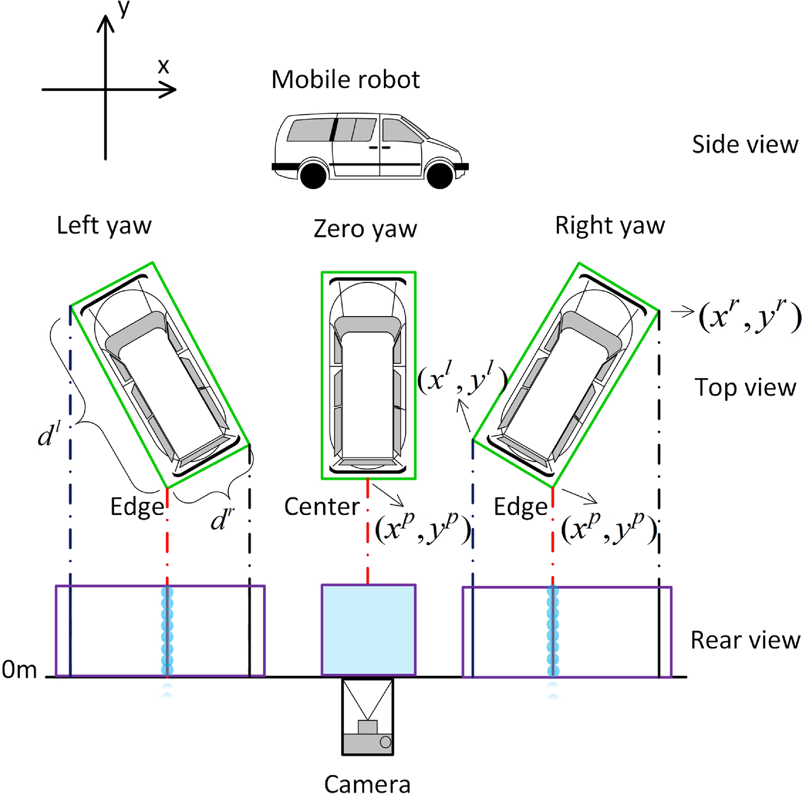
In this study, we suppose the object has rectangular body shown in Figure 1. Suppose that the length denoted by
 $r_l$
and the width denoted by
 $r_w$
w.r.t. the robot are known. Besides, we suppose the orientation
 $\theta _t \in (0,\pi )$
, where for the case
 $\theta _t \in [\!-\!\pi ,0]$
, it can be easily judged through the object’s movement direction. To achieve the pose estimation for such object, we suppose the observation platform can use some sensors (e.g., the RGB-D camera) to get the RGB-D images and velocity odometry information for the object. However, the measurement is usually not correct due to the noise effect and model accuracy. Besides, the real-time performance is very important for practical platform. Considering these points, the goal of this study is to design a real-time pose estimation method together with a good accuracy for the robot object.
Schematic diagram of the observation for the robot in the forward view of the observation platform.

Remark 1. For the observation platform, its pose is usually known. As a result, if it can get the measurement under its own local coordinate system, the global measurement for the object can also be obtained. Without loss of generality, we directly suppose the observation platform has the world coordinate system.
3. Algorithm design
In this section, we will give the complete pose estimation algorithm design.
Let
 $({x^l},{y^l})$
,
 $({x^r},{y^r})$
, and
 $({x^p},{y^p})$
, respectively, represent the leftmost coordinate, the rightmost coordinate and the coordinate with the smallest depth on the robot’s top view in the forward view of the observation platform’s coordinate system (see Figure 1 for details). Obviously, if the orientation
 $\theta \ne \frac {\pi }{2}$
and
 $\theta \in (0,\pi )$
,
 $({x^p},{y^p})$
is unique. Otherwise,
 $({x^p},{y^p})$
may not be unique. For this case, we let
 $({x^p},{y^p})$
represent the relative position from the robot’s tail/head center to the observation platform. Let
 \begin{eqnarray} d^l &=& \sqrt {{{({x^l} - {x^p})}^2} + {{({y^l} - {y^p})}^2}}, \nonumber\\[4pt] d^r &=& \sqrt {{{({x^r} - {x^p})}^2} + {{({y^r} - {y^p})}^2}}. \end{eqnarray}
By (2), it can be concluded that if
 $\theta \ne \frac {\pi }{2}$
and
 $\theta \in (0,\pi )$
,
 ${r_l} = \max \!({d_l},{d_r})$
, and
 ${r_w} = \min\!({d_l},{d_r})$
. Then, if the accurate coordinate information can be obtained, we can obtain the following conclusion.
Proposition 1. Suppose that
 $\theta _t \in (0,\pi )$
and positions
 $({x^l},{y^l})$
,
 $({x^r},{y^r})$
,
 $({x^p},{y^p})$
can be measured accurately. Then, the following statements are true:
-
1. if
 $d^l = d^r$
,
${(x,y,\theta )} = \left({x^p} ,{y^p}+\frac {r_l}{2},\frac {\pi }{2}\right)$
;
-
2. if
$d^l \lt d^r$
,
$(x,y,\theta )= \left( \frac {{{x^l} + {x^r}}}{2}, \frac {{{y^l} + {y^r}}}{2},\arctan \left(\frac {{{y^r} - {y^p}}}{{{x^r} - {x^p}}}\right)\right)$
; -
3. if
$d^l \gt d^r$
,
$(x,y,\theta ) = \left( \frac {{{x^l} + {x^r}}}{2}, \frac {{{y^l} + {y^r}}}{2},\pi +\arctan \left(\frac {{{y^r} - {y^p}}}{{{x^r} - {x^p}}}\right)\right)$
.


Based on Figure 1, the proof can be easily obtained and is omitted here.
To estimate
 $(x,y,\theta )$
for the object, one should first achieve the object detection and then give the pose estimation, where the whole flow chart is illustrated in Figure 2. The first module is object detection. The second module involves pose estimation for objects based on the depth difference information caused by the object’s shape. Finally, Kalman filter is employed to yield smoother and more robust pose estimation results. Detailed descriptions of each module are shown by the following subsections.
Block diagram of the proposed algorithm.

3.1. A lightweight object detection model
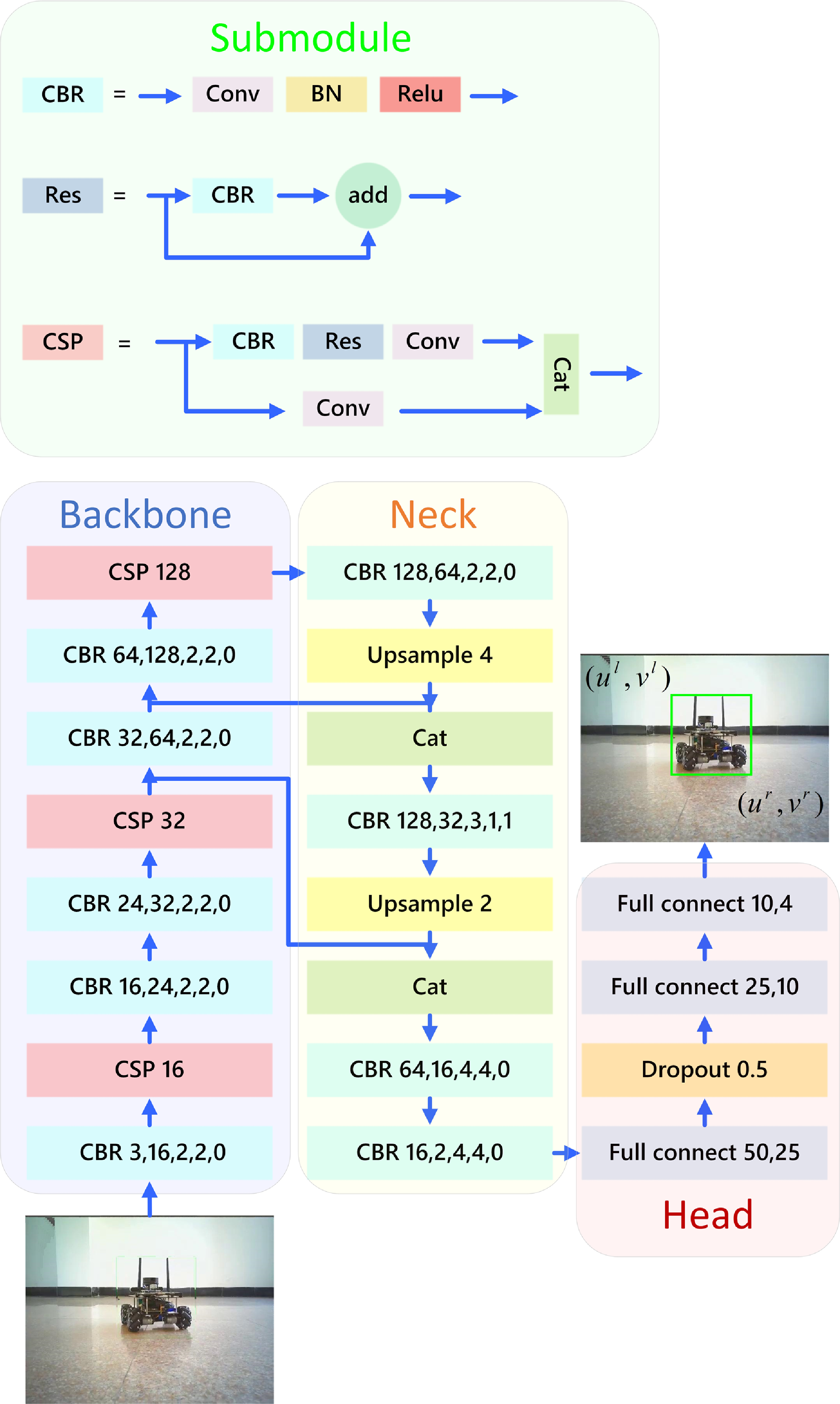
In order to design a lightweight single-object detection model that can run smoothly on embedded platforms, this study designs a one-stage deep learning based object detection model (see Figure 3 for details) inspired by YOLO series [Reference Redmon, Divvala, Girshick and Farhadi25].
A lightweight object detection model.

This model adopts the FPN network structure [Reference Lin, Dollár, Girshick, He, Hariharan and Belongie38], which comprises backbone network, neck network, and detection head. The network uses low-level and high-level features to improve object detection accuracy across scales. For the feature extraction network (i.e., the backbone network), the CBR and CSP modules (shown in the top of Figure 3) are introduced to reduce computational burden while enhancing learning ability. The detailed improvements are shown as follows:
-
1. integrating CSP modules to reduce computational burden while enhancing learning ability.
-
2. gradually increase the number of convolutional channels to avoid instability during training.
-
3. downsampling with convolutional kernel size and stride of 2 to extract high-level semantic information.
-
4. using the feature fusion under top-down propagation and lateral connections to ensure rich semantic and precise positioning.
Unlike traditional object detection, this study focuses solely on single-object detection, where the evaluation relies solely on the CIoU Loss function.
3.2. Direct pose estimation based on RGB-D images
In this part, we will introduce a method to estimate the pose for the mobile robot object based on RGB-D images.
Let
 $(u,v)$
represent the pixel coordinate in the image coordinate system with
 $f(u,v)$
being the corresponding depth. The transformation from image coordinates
 $(u,v)$
to world coordinates
 $(x,y,z)$
can be expressed as [Reference Kenney and McDaniel39]
 \begin{equation} [x,y,z]^T = {K^{-1}}*[u,v,1]^T*f(u,v), \end{equation}
where
 $K$
represents the intrinsic matrix of the depth camera. Let
 $(u^l, v^l)$
and
 $(u^r, v^r)$
, respectively, represent the upper left and lower right corners of the anchor box w.r.t. the object (see the output of the detection model in Figure 3 for details).
First, we will give the estimation for coordinates
 $({x^p},{y^p})$
,
 $({x^l},{y^l})$
, and
 $({x^r},{y^r})$
. Let
 $U^p$
represent a set consisting of all
 $u$
-axis coordinates with the smallest depth, where each element can be obtained through the following formula:
 \begin{equation} u = \mathop {\arg \min }\limits _{u \in [{u^l},{u^r}]} f(u,v),\forall v \in [{v^l},{v^r}]. \end{equation}
Let
 $\mu ^p$
and
 $\delta ^p$
, respectively, denote the sample mean and variance w.r.t. the elements in
 $U^p$
, which are calculated as
 \begin{equation} \mu ^p = \frac {1}{|U^p|} \sum _{u \in U^p} u, \quad \delta ^p = \frac {1}{|U^p|} \sum _{u \in U^p} (u - \mu ^p)^2. \end{equation}
Then,
 $(x^p,y^p)$
can be estimated by (3) with
 $(u,v) = ({\mu ^p},\frac {{{v^l} + {v^r}}}{2})$
. Let
 $U^l$
represent a set of 3D points
 $(x, y, z)$
corresponding to pixels in the depth image. These points are computed by applying the transformation in (3) to all pixel coordinates
 $(u, v)$
that satisfy the following conditions: (1)
 $u \in [u^l, \mu ^p]$
, that is, along the horizontal axis from the leftmost edge of the detected bounding box to the intermediate reference point with minimum depth; (2)
 $v = \frac {v^l + v^r}{2}$
, which corresponds to the vertical midpoint of the bounding box; and (3) the associated depth value
 $f(u, v)$
is valid (i.e., non-null). That is,
 $U^l$
consists of all valid 3D points along the horizontal line at the center of the bounding box, from the left boundary to the point of minimal depth. Then, the point
 $(x^l, y^l, z^l)$
can be estimated as the 3D point in
 $U^l$
with the minimum
 $x$
-coordinate:
 \begin{equation} (x^l,y^l,z^l) = \mathop {\arg \min }\limits _{(x,y,z) \in {U^l}}\,\, x. \end{equation}
Let
 $U^r$
represent a set w.r.t.
 $(x,y)$
, where each element is obtained by (3) with
 $u \in [{\mu ^p},{u^r}]$
and
 $v= \frac {{{v^l} + {v^r}}}{2}$
while satisfies that the obtained depth value
 $z$
is no-null. Then,
 $(x^r,y^r)$
can be estimated through the similar computation for (6) with
 \begin{equation} (x^r,y^r,z^r) = \mathop {\arg \max }\limits _{(x,y,z) \in {U^r}}\,\, x. \end{equation}
Second, we will adopt the least square method to give the orientation estimation. Based on the estimated
 $({x^p},{y^p})$
,
 $({x^l},{y^l})$
and
 $({x^r},{y^r})$
, we can obtain the estimation of
 $d^l$
and
 $d^r$
by (2). Given the linear regression equation
 $f(x)=kx+b$
, then, we can obtain two pairs of the estimation w.r.t.
 $(k, b)$
by solving the following least square problem:
 \begin{equation} \left \{ \begin{array}{l} ({k^r},{b^r}) = \mathop {\arg \min }\limits _{k,b} \sum \limits _i {{{(\,f({x^i}) - {y^i})}^2}} ,s.t.({x^i},{y^i}) \in {U^r}, \\[3pt] ({k^l},{b^l}) = \mathop {\arg \min }\limits _{k,b} \sum \limits _i {{{(\,f({x^i}) - {y^i})}^2}} ,s.t. ({x^i},{y^i}) \in {U^l}. \end{array} \right. \end{equation}
The above optimization problems have closed-form solutions with
 \begin{equation} k = \frac {\sum _i (x^i - \bar {x})(y^i - \bar {y})}{\sum _i (x^i - \bar {x})^2}, \quad b = \bar {y} - k\bar {x}, \end{equation}
where
 $\bar {x}$
and
 $\bar {y}$
denote the sample means of the
 $x^i$
and
 $y^i$
values in
 $S$
, respectively. Then, the orientation
 $\theta$
can be estimated as
 \begin{equation} \theta = \left \{ \begin{array}{l} \arctan \!({k^r}),\qquad\quad\,\,\,\,\, \text{if}{d^l} \lt {d^r}, \\ \pi + \arctan \!({k^l}),\qquad\text{otherwise}. \end{array} \right. \end{equation}
Finally, we can estimate the object coordinates as follows. When the orientation is orthogonal (i.e.,
 $\theta = \frac {\pi }{2}$
), the center is set to
 $(x^p, y^p + \frac {r_l}{2})$
. For non-orthogonal cases, as stated in Proposition 1, the left and right boundaries are fitted as lines
 $y = k^l x + b^l$
and
 $y = k^r x + b^r$
. The horizontal coordinate is estimated as the midpoint
 $(x^l + x^r)/2$
, while the vertical coordinate is given by the average of the two fitted lines at the corresponding endpoints. The final expression is
 \begin{equation} (x,y) = \left \{ \begin{array}{ll} \left(x^p, y^p + \frac {r_l}{2}\right), & \quad \text{if}\,\, \theta = \frac {\pi }{2}, \\[6pt] \left ( \frac {x^l + x^r}{2}, \frac {k^l x^l + b^l + k^r x^r + b^r}{2} \right ), & \quad \text{otherwise}. \end{array} \right. \end{equation}
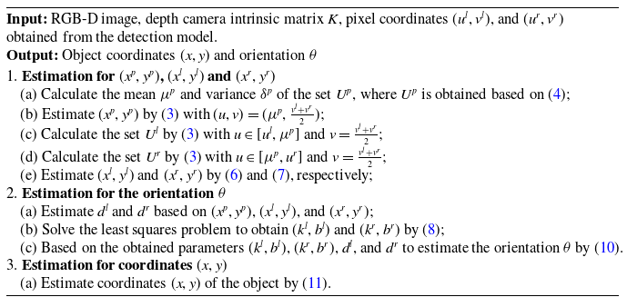
Now, the RGB-D image-based pose estimation algorithm is summarized in Algorithm 1.
The implementation of the RGB-D image based pose estimation algorithm
Input: RGB-D image, depth camera intrinsic matrix
 $K$
, pixel coordinates  $(u^l, v^l)$
, and  $(u^r, v^r)$ |
| obtained from the detection model. |
Output: Object coordinates
 $(x, y)$
and orientation  $\theta$ |
1. Estimation for
 $(x^p, y^p)$
,  $(x^l, y^l)$
and  $(x^r, y^r)$ |
(a) Calculate the mean
 $\mu ^p$
and variance  $\delta ^p$
of the set  $U^p$
, where  $U^p$
is obtained based on (4); |
(b) Estimate
 $(x^p, y^p)$
by (3) with  $(u, v) = (\mu ^p, \frac {v^l + v^r}{2})$
; |
(c) Calculate the set
 $U^l$
by (3) with  $u \in [{u^l},{\mu ^p}]$
and  $v= \frac {{{v^l} + {v^r}}}{2}$
; |
(d) Calculate the set
 $U^r$
by (3) with  $u \in [{\mu ^p},{u^r}]$
and  $v= \frac {{{v^l} + {v^r}}}{2}$
; |
(e) Estimate
 $(x^l, y^l)$
and  $(x^r, y^r)$
by (6) and (7), respectively; |
2. Estimation for the orientation
 $\theta$ |
(a) Estimate
 $d^l$
and  $d^r$
based on  $(x^p, y^p)$
,  $(x^l, y^l)$
, and  $(x^r, y^r)$
; |
(b) Solve the least squares problem to obtain
 $(k^l, b^l)$
and  $(k^r, b^r)$
by (8); |
(c) Based on the obtained parameters
 $(k^l, b^l)$
,  $(k^r, b^r)$
,  $d^l$
, and  $d^r$
to estimate the orientation  $\theta$
by (10). |
3. Estimation for coordinates
 $(x,y)$ |
(a) Estimate coordinates
 $(x, y)$
of the object by (11). |

3.3. Pose estimation by fusing odometry data
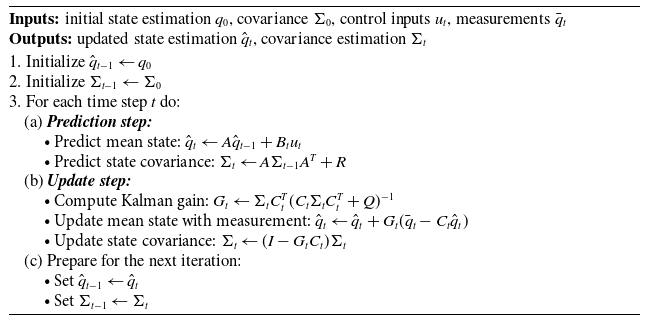
If object’s odometry data can be achieved by the observation platform, a Kalman filter-based pose estimation can be further constructed to improve the robustness and accuracy. The detailed algorithm is shown in Algorithm 2.
Kalman filter based pose estimation by fusing odometry data
Inputs: initial state estimation
 $q_0$
, covariance  $\Sigma _0$
, control inputs  $u_t$
, measurements  $\bar q_t$ |
Outputs: updated state estimation
 $\hat {q}_t$
, covariance estimation  $\Sigma _t$ |
1. Initialize
 $\hat {q}_{t-1} \gets q_0$ |
2. Initialize
 $\Sigma _{t-1} \gets \Sigma _0$ |
3. For each time step
 $t$
do: |
| (a) Prediction step: |
• Predict mean state:
 ${\hat {q}}_t \gets A \hat {q}_{t-1} + B_t u_t$ |
• Predict state covariance:
 ${\Sigma }_t \gets A \Sigma _{t-1} A^T + R$ |
| (b) Update step: |
• Compute Kalman gain:
 $G_t \gets {\Sigma }_t C_t^T (C_t {\Sigma }_t C_t^T + Q)^{-1}$ |
• Update mean state with measurement:
 $\hat {q}_t \gets {\hat {q}}_t + G_t (\bar q_t - C_t {\hat {q}}_t)$ |
• Update state covariance:
 $\Sigma _t \gets (I - G_t C_t) {\Sigma }_t$ |
| (c) Prepare for the next iteration: |
• Set
 $\hat {q}_{t-1} \gets \hat {q}_t$ |
• Set
 $\Sigma _{t-1} \gets \Sigma _t$ |

In this algorithm, definitions of
 $A$
,
 $B_t$
, and
 $u_t$
are given (1).
 ${C_t}=I$
is the observation matrix.
 $\Sigma _0$
represents the corresponding covariance matrix of
 $\hat q_0$
, which is set as a zero matrix.
 $\bar q_t=[x_t,y_t,\theta _t]^T$
represents the estimation values obtained by Algorithm 1. The covariance matrices
 $R$
and
 $Q$
are set as follows:
 \begin{equation} {R} = \left[\begin{array}{c@{\quad}c@{\quad}c} r^x & 0 & 0 \\ 0 & r^y & 0 \\ 0 & 0 & r^\theta \\ \end{array}\right],\quad {Q} = \left[\begin{array}{c@{\quad}c@{\quad}c} q^x & 0 & 0 \\ 0 & q^y & 0 \\ 0 & 0 & q^\theta \\ \end{array}\right], \end{equation}
where the parameters
 $r^x, r^y, r^\theta$
and
 $q^x, q^y, q^\theta$
are estimated by the sample variance of the odometry data and the pose obtained by Algorithm 1, respectively. Here, a pre-experiment sampling process can be conducted to complete the estimation.
4. Simulation and experiment
4.1. Model performance comparison
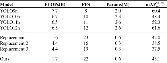
To highlight the lightness and rapidity of the propose model in this paper, comparative experiments are conducted with the lightweight models in recently proposed YOLO series detection model, specifically the YOLO9n [Reference Wang, Yeh and Liao27], YOLO10n [Reference Wang, Chen, Liu, Chen, Lin, Han and Ding40], YOLO11n [Reference Khanam and Hussain41], and YOLO12n [Reference Tian, Ye and Doermann42] model. The entire experiments are carried out on a Jetson Nano with 4 GB of memory. Various indicators were used to measure the time complexity, space complexity, and detection accuracy of each model. The specific details are shown in Table I.
Model performance comparison.

From Table I, it is evident that while our model exhibits a marginal accuracy trade-off compared to state-of-the-art algorithms, its parameter count and computational requirements are reduced to only one-fourth of other models. This optimization enables the model to achieve double the inference speed in embedded systems, effectively satisfying real-time application requirements.
To further validate the effectiveness of the proposed architecture, we conduct an ablation study by performing the following module replacements:
-
1. replacing CSP modules with convolutional layers of equal depth.
-
2. using a fixed number of channels throughout the backbone instead of gradual channel increment.
-
3. considering both (1) and (2) simultaneously.
As shown in Table I, the proposed model achieves the highest mAP
 $_{\text{val}}^{50\text{-}95}$
of 43.1 with relatively low computational cost and a compact parameter size, indicating a favorable balance between accuracy and efficiency. In comparison, while replacement (1) has a similar model size, it sacrifices some accuracy. Replacements (2) and (3), in contrast, are more computationally expensive and yet exhibit lower performance due to the removal of the gradual channel increment. These results demonstrate that the overall architectural design of the proposed model is better suited for lightweight object detection.
4.2. Simulation
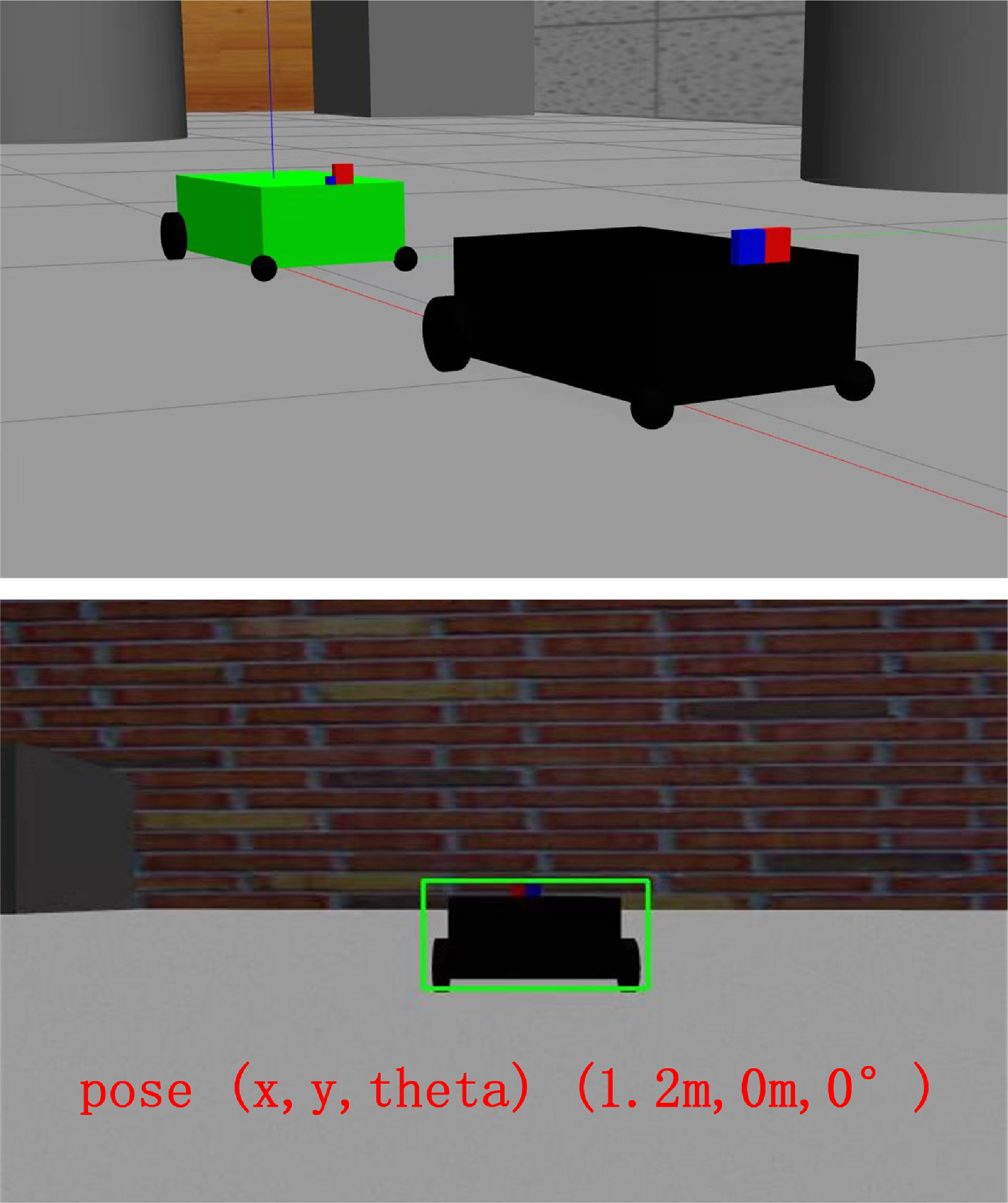
First, a numerical simulation that contains two mobile robots with one leader and one follower is conducted in Gazebo shown in Figure 4, where the follower will make the pose estimation for the leader. Initial poses of the leader and follower are, respectively, set as
 $(1.2m, 0m, 0^\circ )$
and
 $(0m, 0m, 0^\circ )$
. The depth measurement and odometry information are supposed to be disturbed by Gaussian noises that both follow
 $N(0,0.1)$
. The sampling interval of the RGB-D camera is set to 30 ms. For visual detection, the maximum and minimum detection ranges are set to 5 and 1 m, respectively. The horizontal field of view of the camera is set as
 $60^ \circ$
.
Simulation in Gazebo with a black leader robot and a green follower robot.

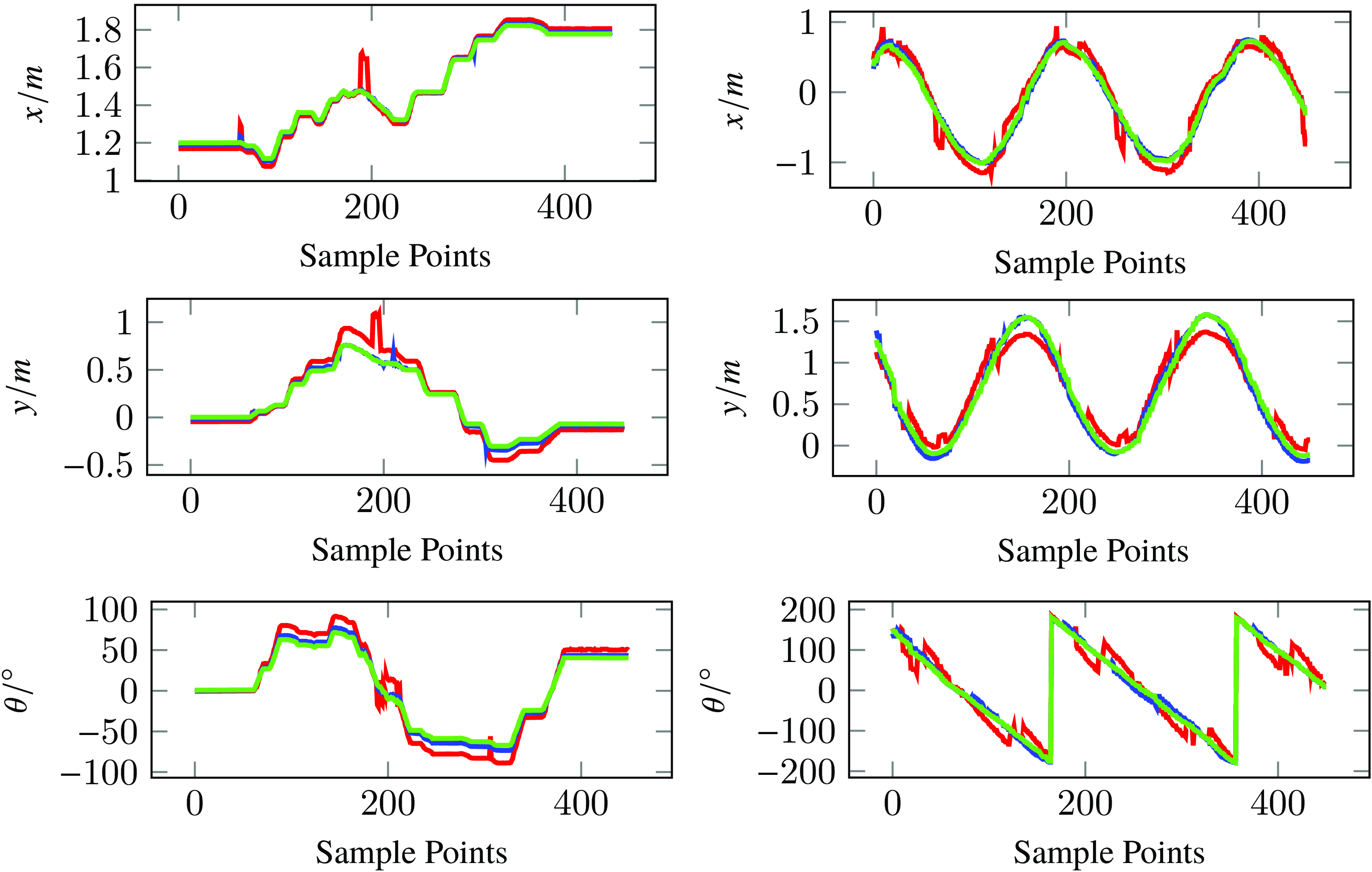
Let the leader robot, respectively, move along an S-shaped curve and circular curve. Then, under the pose estimation Algorithms 1 and 2, we can obtain the simulation result shown by Figure 5. From Figure 5, we can see that if the pose information can be obtained in real time, both Algorithms 1 and 2 can achieve a good estimation performance, which validates the effectiveness of the algorithms. However, Algorithm 2 will be more robust if the measure error is very big. To further verify this point, mean absolute error (MAE), maximum error, and minimum error are used to evaluate the performance of Algorithms 1 and 2. By comparing both algorithms with the actual values, the error analysis is given in Tables II and III. It can be seen that Algorithm 2 achieves lower MAE (e.g., 0.0068 vs. 0.0258 for
 $x/m$
in S-shape, 0.0287 vs. 0.1153 for
 $x/m$
in circular) and smaller maximum errors (e.g., 0.1266 vs. 0.4939 for
 $y/m$
in S-shape, 0.1124 vs. 0.2924 for
 $y/m$
in circular) compared to Algorithm 1. Through this analysis, we can see that the Kalman filter based pose estimation by fusing odometry data can achieve better accuracy and robustness, especially under large measurement errors.
Error analysis of S-shape route.

Error analysis of circular route.


4.3. Experimental result
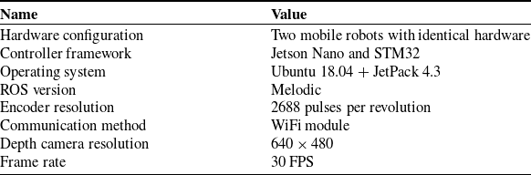
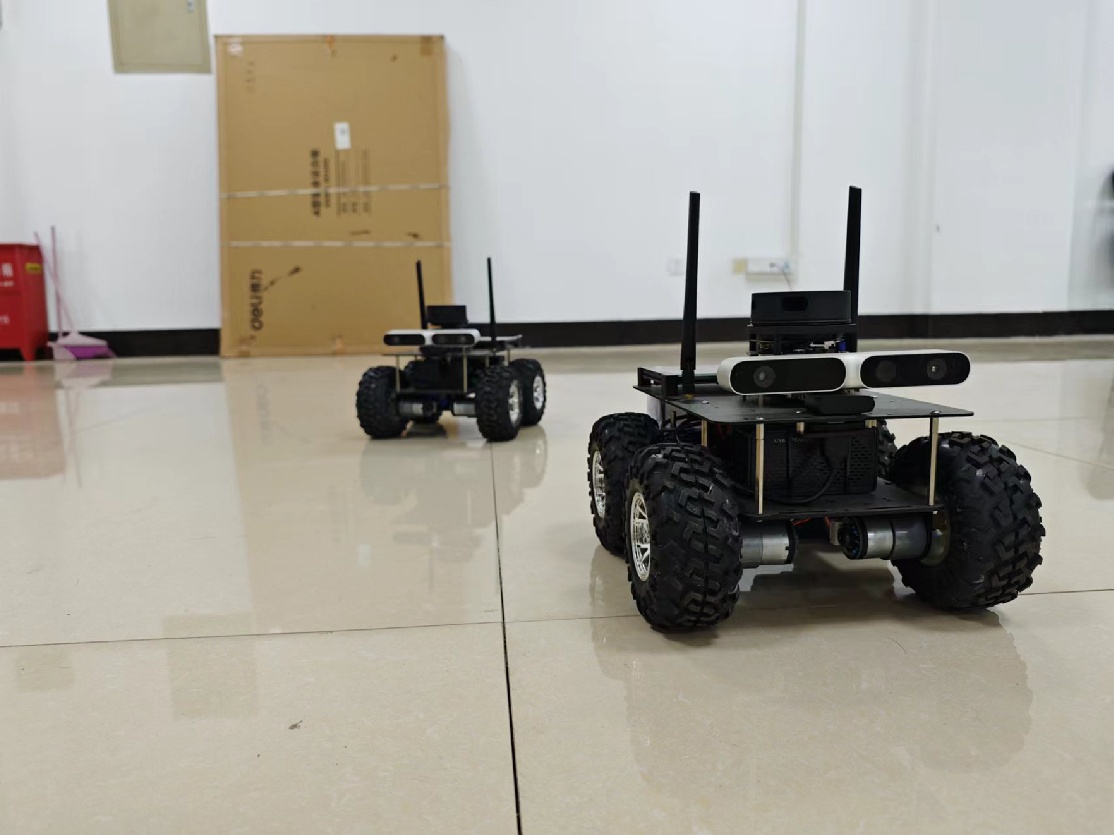
In this part, we will conduct an experiment in actual physical platform to further investigate the performance of our algorithm. The platform contains two intelligent mobile robots depicted in Figure 6. The specific equipment involved in the experiment is shown in Table IV.
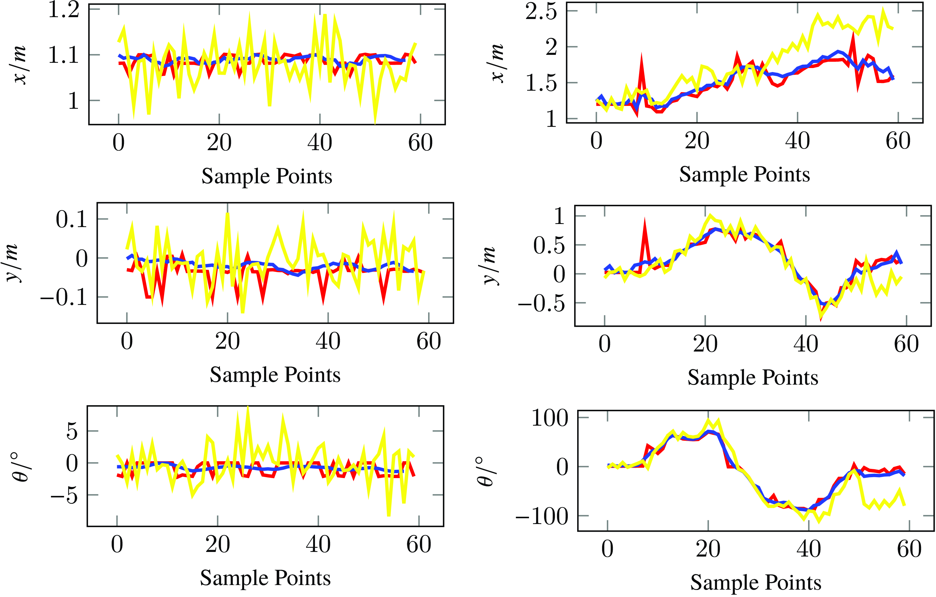
Let the leader robot, respectively, be stationary and move along an S-shaped curve. Then, under Algorithms 1 and 2, we can obtain the experiment result shown by Figure 7. From Figure 7, we can see that the odometry information exists a big error, especially if the robot is moving, while both Algorithms 1 and 2 can achieve a good estimation performance at speeds exceeding 20 FPS. This experiment further validates the effectiveness of the proposed algorithm.
Remark 2. Due to the uncertainties in the estimation process, such as the measurement error, image quality, estimation errors are inevitable. For example, two vectors
 $(x^p-x^l, y^p-y^l)$
and
 $(x^p-x^r, y^p-y^r)$
are orthogonal theoretically for the left/right yaw case shown in Figure 1, but in practice they may not. Here, the estimation of parameters is computed directly based on the Algorithms 1, 2 with the formular given in Subsection 3.2, and we only adopt the following strategy to improve the robustness and precision during the estimation progress: when the object detection module occasionally fails, the pose estimation is skipped for the current frame and the previous pose is used as a temporary approximation. Other scenarios, such as odometry data loss, have not been considered in our algorithm. Consequently, inadequate measurement data or low-precision sensor inputs may cause complete malfunction of the proposed algorithmic system.
It is evident that the robustness and accuracy of the algorithm still need to be further improved. Regarding potential countermeasures, one can enhance the image quality by incorporating advanced image enhancement techniques [Reference Zhou, Leng, Fang, Xiang, Wei and Jia35, Reference Zhou, Wu, Wei, Xiang, Fang and Kwong36, Reference Guo, Zhang, Zhou, Yue, Pu and Luo43−Reference Guo and Zhou45] and image quality assessment methods [Reference Zhou, Lan, Wei, Liao, Mao, Li, Wu, Xiang and Fang46−Reference Shen, Zhou, Luo, Li and Kwong48]. Besides, several fault-tolerance strategies and data filtering methods need to be further developed to inhibit the drift or error of the measurement data.
Experimental facilities.

Experimental setup.

5. Conclusion
In this study, two algorithms have been proposed to solve the real-time pose estimation problem for a class of mobile robots with rectangular body. It should be noted that the algorithm can be easily extended to other kinds of robots with a certain geometry body as long as the pose can be uniquely determined. Both simulation and experiment show that the proposed algorithm can achieve the good performance in terms of real-time performance and accuracy.

Note that Algorithm 2 proposed in this paper depends on the velocity odometry data, which is supposed that it can be directly obtained by the follower. However, in practice, the assumption is hard to be satisfied. In addtion, the environment considered in this study is relatively simple, We have not taken into consideration scenarios that involve obstacles, potential sensor malfunctions, and the filtering of sensor measurement data. The real-time pose estimation algorithm with higher accuracy and robustness that completely depends on the measurement information in complex environment is a direction of our further work.
Author contribution
Haoran Tang and Bo Wang conceived the study and designed the methodology. Haoran Tang performed the simulation and experiment. All authors contributed to the review and editing of the manuscript.
Financial support
This work was supported by the National Natural Science Foundation of China (under grants 61903110 and 62073108) and Natural Science Foundation of Zhejiang Provincial (under grant LZ23F030004).
Competing interests
The authors declare no conflicts of interest exist.