3.1. Spectra with and without surface roughness

Figure 3 shows the spectra of the initial disturbances excited by each roughness configuration measured at $R=290$ and $z=1.3$ . The solid (black) lines show spectra of the instantaneous (or single-realization) velocity time series from a hot-wire probe, which contain both stationary and unsteady components, and the dashed (red) lines show spectra of the ensemble-averaged velocity time series with the unsteady and travelling components averaged away. Note that the instantaneous velocity time series are the time series of a hot-wire probe in the laboratory frame at a certain radius and wall-normal height, and since the disk is moving relative to the hot-wire probe, the instantaneous velocity time series contain components that are stationary with respect to the disk and unsteady (including travelling-wave) components. The long instantaneous time series were divided into segments of 2048 samples, the spectrum for each sample length was calculated and then finally the (ensemble) average of these spectra is presented (solid line) in each subplot of figure 3. The ensemble-averaged time series were calculated by ensemble-averaging individual instantaneous time series for single revolutions of the disk, and then the dashed lines in figure 3 were calculated by taking the spectra of these ensemble-averaged time series. The ensemble averaging of time series for individual revolutions of the disk, if done over a sufficient number of time series, averages away the unsteady components that are not repeatable from one revolution to the next, leaving only those components that are repeatable, i.e. those that are fixed relative to the disk, namely the stationary components.

The peak at around ${\it\omega}^{\ast }/{\it\Omega}^{\ast }=1$ is due to the small rotational imbalance of the disk, where ${\it\omega}^{\ast }$ is the disturbance frequency in the laboratory frame. Figure 3(a) shows a clear peak in both spectra at ${\it\omega}^{\ast }/{\it\Omega}^{\ast }=32$ attributed to the 32 roughnesses, which produce disturbances that are stationary in the rotating-disk frame and, therefore, give rise to oscillations 32 times per revolution of the disk in the laboratory frame. (Note that in the rotating frame, the 32 oscillations that are fixed relative to the disk correspond to azimuthal wavenumbers of 32 and zero disturbance frequencies.) Furthermore, it is also shown that the roughnesses excite not only ${\it\omega}^{\ast }/{\it\Omega}^{\ast }=32$ but also other stationary modes. These spiky peaks are attributed to a superposition of unstable stationary disturbances across a range of azimuthal integer wavenumbers (in the rotating frame), as explained in the appendix of Imayama et al. (Reference Imayama, Alfredsson and Lingwood2014). As the number of roughnesses is decreased from 24 to 8, the mode with ${\it\omega}^{\ast }/{\it\Omega}^{\ast }=32$ is still excited but with decreasing relative amplitude compared with other frequencies. With a single roughness element, no peak at ${\it\omega}^{\ast }/{\it\Omega}^{\ast }=32$ is observed. This is because a single roughness element excites all wavenumbers (some growing and some decaying) and not any particular mode. With a clean disk, the stationary-disturbance amplitude indicated by the dashed line is very small compared with other cases. The peaks around ${\it\omega}^{\ast }/{\it\Omega}^{\ast }=67$ in the spectra of instantaneous time series for the clean-disk condition and other cases are due to electrical noise from the inverter. Unlike most of the clean-disk data presented in this paper, the data for $R=290$ in figure 3(f) were measured after the roughness experiments were completed.

3.2. Azimuthal mean velocity profiles

The measured azimuthal mean velocity profiles with 32 roughness elements are shown in figure 4(a) and the deviations of the mean velocity profiles from the theoretical laminar azimuthal profile are shown in figure 4(b). At low Reynolds number, there is close agreement between the measured azimuthal mean velocity profiles and the theoretical profile. The experimental non-dimensional boundary-layer thickness, ${\it\delta}_{95}$ , and that for the theoretical laminar profile are shown as a dashed line with squares and a solid line, respectively. At $R=475$ the boundary-layer thickness starts to increase in the vertical (wall-normal) direction. At higher Reynolds number, the boundary layer grows rapidly and the azimuthal velocity profile deviates from the theoretical one as shown in figure 4(b), and at $R=555$ the velocity profile indicates a turbulent boundary layer. Although not presented in this paper, the azimuthal mean velocity profiles have been measured for 16 and 8 roughness elements ([1–8, 25–32], [1–8]) at $R=395$ , and those measurements confirm that the profiles match the theoretical laminar profile.

Figure 4.

(a) Profiles of azimuthal mean velocity, $V$ , (in the laboratory frame) and (b) deviation of azimuthal mean velocity from the theoretical laminar profile, ${\rm\Delta}V$ . Profiles measured for cases PP01R32–12R32 at (A)  $R=335$ , (B)  $R=355$ , (C)  $R=375$ , (D)  $R=395$ , (E)  $R=415$ , (F)  $R=435$ , (G)  $R=455$ , (H)  $R=475$ , (I)  $R=495$ , (J)  $R=515$ , (K)  $R=535$ , (L)  $R=555$ . The solid lines at each Reynolds number show the theoretical azimuthal laminar velocity profiles. The solid line at $z=3.60$ indicates the normalized theoretical boundary-layer thickness for the laminar profile where $V$ becomes 0.05. The squares with the dashed lines show the measured boundary-layer thickness ( ${\it\delta}_{95}$ ) given in table 1.

Imayama et al. (Reference Imayama, Alfredsson and Lingwood2014) show azimuthal mean velocity profiles for the clean-disk condition at various Reynolds number in their figure 2. In comparison, it is recognized that the transition to turbulence with 32 roughness elements occurs at lower Reynolds number. In particular, the growth of the boundary-layer thickness starts at about $R=475$ , which is lower than the onset of local absolute instability, i.e.  $R_{CA}=507$ . Lingwood (Reference Lingwood1995) suggested that the local absolute instability triggers the onset of nonlinearity and transition. However, in this case, the 32 roughness elements produce relatively large-amplitude stationary disturbances in the flow field, as shown in figure 3(a), and Type-I stationary cross-flow instabilities grow sufficiently to trigger the onset of nonlinearity at $R<R_{CA}$ . This route to laminar–turbulent transition therefore looks to be via a convectively unstable process, and occurs at lower Reynolds number than for a clean disk.

Figure 5.

The rotating-disk boundary-layer characteristics as functions of Reynolds number on a log–log scale: ▫, the boundary-layer thickness, ${\it\delta}_{95}^{\ast }$ ; ▵, the displacement thickness, ${\it\delta}_{1,95}^{\ast }$ ; ♢, the momentum thickness, ${\it\delta}_{2,95}^{\ast }$ ; ○, the shape factor, $H_{95}$ . The solid line shows the theoretical shape factor, $H_{95}=2.23$ , based on the boundary-layer thickness ${\it\delta}_{95}^{\ast }$ . Obtained from the same data as in figure 4.

Rapid growth of the boundary-layer thickness is observed at around $R=495{-}515$ . Since the mean azimuthal velocity is calculated by azimuthally averaging instantaneous velocity measurements, the rapid growth indicates that the azimuthal variations of the transition process are small, which may be expected given that this case (PP01R32–PP12R32) is controlled by an axi-symmetric array of the 32 roughness elements, see figure 2(a). As discussed later, breaking the symmetry of the surface roughnesses by removing some of them causes azimuthal variation in the transition process. However, this rapid growth in ${\it\delta}_{95}$ is also observed in the clean-disk condition, see figure 2(a)(I, J) in Imayama et al. (Reference Imayama, Alfredsson and Lingwood2014). Furthermore, Imayama et al. (Reference Imayama, Alfredsson and Lingwood2014) reported, for a clean disk, on the growth of both stationary and travelling instabilities in the transition regime, and showed that the stationary vortices break down independently of their individual amplitudes at around $R=585$ . So, while the boundary layers for the axi-symmetric rough disk and for the clean disk both show rapid growth, we hypothesize that this behaviour may be attributed to different transition mechanisms. Further analysis of the stationary vortices for the rough-disk condition is discussed in § 3.3.

Figure 5 shows the boundary-layer parameters using a log–log scale; these are also shown in table 1. One of the characteristics of the similarity solution of the infinite-radius rotating-disk boundary-layer flow is that the boundary-layer thickness is constant independent of radius at fixed rotational speed and kinematic viscosity, and equivalently independent of $R$ . In Imayama et al. (Reference Imayama, Alfredsson and Lingwood2014) velocity profile measurements were made at a fixed radial position and the Reynolds number was changed by varying the rotational speed. In the present study, a constant boundary-layer thickness was observed at low Reynolds numbers since the rotational speed was fixed and different Reynolds numbers were obtained by varying the local radial location of the hot-wire probe. The obtained shape factor, $H_{95}$ , between $R=335$ and $R=455$ is in good agreement with the theoretical value, $H_{95}=2.23$ , shown as a solid line. Above $R=475$ , the boundary-layer thickness, displacement thickness and momentum thickness start increasing whereas the shape factor decreases. The shape factor at $R=555$ reaches 1.42 and it is similar to the value at $R=630$ for the clean-disk condition and in good agreement with Cham & Head’s (Reference Cham and Head1969) measurement results for a turbulent rotating-disk boundary-layer flow, as discussed in Imayama et al. (Reference Imayama, Alfredsson and Lingwood2014).

3.3. Velocity-disturbance characteristics

Measurements of the disturbance amplitude were performed for various roughness configurations and at $z=1.3$ with intervals of ${\rm\Delta}R=5$ to investigate the laminar–turbulent transition process. To maximize the signal-to-noise ratio as in Imayama et al. (Reference Imayama, Alfredsson and Lingwood2014), the signals were filtered with a bandpass filter $17<{\it\omega}^{\ast }/{\it\Omega}^{\ast }<70$ below $R\leqslant 415$ and with a high-pass filter $17<{\it\omega}^{\ast }/{\it\Omega}^{\ast }$ for $420\leqslant R\leqslant 450$ for IP01R01–IP01R32 and PP01R32–PP06R32, where ${\it\omega}^{\ast }$ is the signal frequency. The disturbance amplitude was calculated as the root-mean-square (r.m.s.) of the instantaneous velocity time series of the azimuthal fluctuation, $v_{rms}^{\ast }$ , normalized by the local disk velocity, $v_{rms}=v_{rms}^{\ast }/(r^{\ast }{\it\Omega}^{\ast })$ , and is plotted in figure 6.

Figure 6 shows the roughness elements located at $R=287$ producing stationary disturbances and $v_{rms}$ increasing from $R=285$ to a peak at $R=295$ . The measured amplitude of the initial excitation around $R=295$ depends on the number of roughnesses. Once the initial excitation of $v_{rms}$ has decreased beyond the roughness elements, the disturbances start increasing exponentially at around $R=330$ . Linear stability analysis (conducted in the rotating frame) shows that stationary disturbances ( ${\it\omega}=0$ ) with azimuthal wavenumber ${\it\beta}=32$ become unstable at around $R=322$ . For 32 roughnesses (IP01R32) the slope of $v_{rms}$ in figure 6 changes at around $R=455$ and a maximum in $v_{rms}$ is found at $R=510$ . As the number of roughnesses is decreased the Reynolds number of the maximum $v_{rms}$ increases, approaching the clean-disk value, and also the maximum amplitudes change.

Figure 6.

The $v_{rms}$ distributions measured at $z=1.3$ with roughnesses: red solid line, 32 roughnesses [1–32]; black solid line, 24 roughnesses [1–8, 17–32]; blue solid line, 16 roughnesses [1–8, 25–32]; green solid line, 8 roughnesses [1–8]; magenta solid line, 1 roughness [8]; black dashed line, 0 roughnesses (clean-disk condition).

Figure 7.

(a) Spectra $P({\it\omega}^{\ast })$ of instantaneous time series for case IP01R32; (b) radial growth rate, $-{\it\alpha}_{i}$ , derived from (a). The $y$ -axis shows normalized frequency (in the laboratory frame) and equivalently (provided the disturbances are fixed relative to the rotating disk) azimuthal wavenumber, ${\it\beta}$ , from local stability theory (in the rotating frame). Thick black solid lines show the theoretical neutral curve inside of which the flow is convectively unstable, $-{\it\alpha}_{i}>0$ , i.e. there is radial spatial growth of stationary disturbances. Solid lines show radial spatial growth rates of $-{\it\alpha}_{i}=0.01$ , 0.02, 0.03, 0.04, 0.05 from left to right. The chain line at $R=287$ shows the Reynolds number location of the roughnesses. The dashed line at $R=415$ indicates the onset of nonlinearity for this case.

To compare the growth of stationary disturbances generated by 32 roughness elements with local linear stability analysis, figure 7(a) shows a contour plot of the spectra from instantaneous velocity time series of the azimuthal fluctuation for the case IP01R32. The spectrum at each measurement Reynolds number has spiky peaks at each integer value of ${\it\omega}^{\ast }/{\it\Omega}^{\ast }$ , so the maximum amplitude at each integer ${\it\omega}^{\ast }/{\it\Omega}^{\ast }$ was selected and plotted in figure 7(a). It is assumed that the spectra of the instantaneous time series in this figure are mainly attributable to stationary disturbances excited by roughness elements shown as spiky peaks in figure 3(a).

The chain line in figure 7 shows the location of the roughness elements, $R=287$ . The thick solid line denotes the neutral stability curve for stationary disturbances from local linear stability analysis using Lingwood’s (Reference Lingwood1995) code. For stationary disturbances, ${\it\omega}^{\ast }/{\it\Omega}^{\ast }$ from the experiments corresponds to ${\it\beta}$ in the linear theory. The strong peak at ${\it\omega}^{\ast }/{\it\Omega}^{\ast }=32$ is due to the 32 surface roughnesses. Growth of other azimuthal modes ${\it\omega}^{\ast }/{\it\Omega}^{\ast }=20{-}30$ is also observed, since the surface roughnesses at $R=287$ excite not only ${\it\omega}^{\ast }/{\it\Omega}^{\ast }=32$ but also other azimuthal wavenumbers as shown in figure 3(a). The growth of stationary disturbances is observed in the unstable region, i.e. inside the neutral curve. Figure 7(b) shows the radial growth rate, $-{\it\alpha}_{i}$ , calculated as ${\rm\Delta}\text{ln}\,v_{rms}/{\rm\Delta}R$ , using ${\rm\Delta}R=20$ for each ${\it\omega}^{\ast }/{\it\Omega}^{\ast }$ , from the spectra in figure 7(a). At around $R=287$ the growth of disturbances is high due to the initial excitation but the modes outside the neutral curve are damped after the initial excitation. For $R=300{-}415$ the observed growth rates are in excellent agreement with local linear stability theory both in terms of the distribution of unstable modes and quantitatively, as shown by comparison of the black curves of radial growth rate with the contour levels. In particular, with increasing Reynolds number the highest growth rate shifts to higher ${\it\omega}^{\ast }/{\it\Omega}^{\ast }$ as predicted by the local theory. However, at around $R=415$ , a broad range of frequencies starts growing and the experimental data do not follow local linear stability theory, indicating the onset of nonlinearity. Figure 7(a) also shows harmonics of the primary stationary vortices appearing around ${\it\omega}^{\ast }/{\it\Omega}^{\ast }=64$ . Using the criterion for the onset of nonlinearity given by Imayama et al. (Reference Imayama, Alfredsson and Lingwood2013), the onset of nonlinearity for the 32-roughness case is at $R=415$ , which is significantly lower than $R_{CA}$ , and is here caused by the convective growth of stationary vortices rather than the onset of local absolute instability of travelling disturbances.

To compare disturbance profiles for stationary vortices with eigenfunctions from local stability theory, $v_{rms,st}$ profiles at $R=335,355,375$ and 395 (PP01R32–PP04R32), i.e. in the linear flow region as shown by figure 7, are plotted in figure 8, where the azimuthal disturbance amplitude is obtained from the spectra of the ensemble-averaged velocity time series in the frequency range $31.5<{\it\omega}^{\ast }/{\it\Omega}^{\ast }<32.5$ . The profiles are normalized by the maximum (peak) value. The eigenfunction of the local stationary convective instability ( $R=365$ , ${\it\omega}=0+0.0022\text{i}$ , ${\it\alpha}=0.4388+0\text{i}$ and ${\it\beta}=32$ ) is also plotted as a dashed line. This eigenfunction was calculated using a local linear temporal stability code using Chebyshev polynomial discretization, and was checked against a shooting-method code, which was previously developed by Lingwood (Reference Lingwood1995). The results obtained with the two different methods were found to agree. As can be seen from figure 8, the stationary-disturbance profiles excited by 32 roughness elements are in good agreement with the eigenfunction for Type-I cross-flow stationary vortices predicted by local linear stability theory.

Figure 8.

Profiles of azimuthal disturbance amplitude in the frequency range $31.5<{\it\omega}^{\ast }/{\it\Omega}^{\ast }<32.5$ measured for cases PP01R32–04R32 at $R=335$ (▫), $R=355$ (▵), $R=375$ (○) and $R=395$ (*), i.e. in the linear region. The dashed line is the eigenfunction of the local stationary convective instability ( $R=365$ , ${\it\omega}=0+0.0022\text{i}$ , ${\it\alpha}=0.4388+0\text{i}$ and ${\it\beta}=32$ ). The amplitudes are normalized by the maximum disturbance amplitude.

Figure 9.

Stationary-vortex distributions measured at $z=1.3$ at radial steps of ${\rm\Delta}R=5$ : (a) 32 roughnesses [1–32], (b) 24 roughnesses [1–8, 17–32], (c) 16 roughnesses [1–8, 25–32], (d) 8 roughnesses [1–8]; (e) 1 roughness [8], (f) 0 roughnesses (clean-disk condition). The filled contours from blue to red (colour online) indicate $-0.12$ , $-0.1$ , $-0.08$ , $-0.06$ , $-0.04$ , $-0.02$ , 0, 0.02, 0.04, 0.06, 0.08, 0.1, 0.12 of the ensemble-averaged fluctuation velocity normalized by the local wall speed. The dots indicate locations of roughnesses (the size is not to scale).

Figure 10.

Stationary-vortex characteristics with 32 roughnesses [1–32] measured at $z=1.3$ with a radial step of ${\rm\Delta}R=5$ . (a) Stationary-vortex distributions. The filled contours from blue to red indicate the ensemble-averaged fluctuation velocity normalized by the local wall speed at $-0.12$ , $-0.1$ , $-0.08$ , $-0.06$ , $-0.04$ , $-0.02$ , 0, 0.02, 0.04, 0.06, 0.08, 0.1, 0.12. Dotted lines in (a) indicate $R=300$ , 400, 500, 600, respectively, moving outward. The edge of the disk, i.e.  $R=615$ , is shown as the outer solid circle in (a). The positions of the roughness elements are shown as the black dots (the scale is not actual scale). (b) Each stationary-vortex amplitude, ${\rm\Delta}v_{0.5}$ , where the colour indicates the amplitude of ${\rm\Delta}v_{0.5}$ at $R=350$ . The solid line shows the disturbance amplitude calculated from the radial growth rate of linear stability analysis for ${\it\beta}=32$ ; note that the vertical position is arbitrary. (c) The angle distributions of each stationary vortex, where the colour indicates the reference amplitude shown in (b). The solid line shows the angle predicted by local linear stability analysis for ${\it\beta}=32$ .

Figure 9 shows contour plots of the stationary-disturbance amplitude derived from ensemble-averaged velocity time series (approximately 1000 revolutions/ensemble). The black dots indicate the roughness locations at $R=287$ . With 32 roughnesses (IP01R32), breakdown of the stationary vortices is indicated by the amplitude reduction located at around $R=520$ with no discernible azimuthal variation, which is to be expected given that the amplitudes of the stationary vortices are controlled by the axi-symmetric array of artificial surface roughnesses. For the 32-roughness case the number of stationary vortices is constant (32) from the initial excitation to breakdown. This observation contrasts with earlier experimental observations (e.g. Wilkinson & Malik Reference Wilkinson and Malik1985, Imayama et al. Reference Imayama, Alfredsson and Lingwood2014), which show an increasing number of stationary vortices (usually ranging from about 22 to 32 in the linearly unstable region) as the Reynolds number increases. This is because in the present experiments the 32 mode was preferentially excited (as shown in figure 3) and, despite there being other modes with higher growth rates, the 32 mode maintains the highest amplitude up to breakdown.

Some experimental studies of the rotating-disk boundary-layer flow have captured a low-wavenumber oscillation in the breakdown region, e.g. Kobayashi, Kohama & Takamadate (Reference Kobayashi, Kohama and Takamadate1980), Corke & Knasiak (Reference Corke and Knasiak1998), Imayama et al. (Reference Imayama, Alfredsson and Lingwood2014). However, figure 9(a) does not show this kind of feature in the breakdown region. A discussion of this large-scale stationary structure is given in § 3.4 together with spectra of azimuthal velocity time series.

Removing some of the surface roughness elements results, as shown in figure 9(b–e), in the breakdown locations of the stationary vortices moving downstream and approaching the clean-disk condition in figure 9(f). The convective behaviour of the stationary vortices generated by the roughness elements is clearly shown by figure 9. The angular variations in the azimuthal wavenumber in regions excited by the artificial roughnesses compared with regions not artificially excited are also evident in figure 9(b–d) at around $R=287$ . The naturally most unstable stationary azimuthal wavenumber at the onset of convective instability is around ${\it\beta}=22$ , which is close to the wavenumber observed in figure 9(b–d) at low $R$ in the gap between roughnesses.

In the breakdown and turbulent regions in figure 9(b–e) a large-scale stationary structure is captured. The azimuthal location of the structure seems to be dependent on the positioning of the roughness elements, and particularly linked to the leading roughness element. Figure 9(b–e) shows that the azimuthal position of the large structure shifts to the right (positive ${\it\theta}$ direction) as the leading roughness position moves in the same direction (namely, linked to roughness numbers 17 in (b), 23 in (c), 1 in (d) and 8 in (e)).

Figure 10(a) shows the same data as in figure 9(a) but in the circular geometry, namely stationary disturbances from ensemble-averaged velocity time series of the azimuthal fluctuation at $z=1.3$ with 32 roughness elements (IP01R32). Black dots indicate the locations of the roughness elements. The amplitude of the stationary disturbances reaches a maximum at around $R=500$ and then decreases as the stationary vortices break down. Figure 10(a) is comparable with figure 12(a) in Imayama et al. (Reference Imayama, Alfredsson and Lingwood2014), which also shows stationary disturbances but for the clean disk. In both cases, very little azimuthal variation is observed, but here that is due to the controlling effect of the 32 roughness elements located in an equi-angular arrangement. While also largely independent of angular position, this is in contrast to the mechanism depicted in figure 12(a) in Imayama et al. (Reference Imayama, Alfredsson and Lingwood2014) for the clean disk where the stationary vortices break down independently of their amplitude but at a fixed $R$ . Figure 10(b) shows peak-to-peak amplitudes of each stationary vortex, ${\rm\Delta}v_{0.5}$ , measured at $z=1.3$ ; the same quantity is presented in figure 13(a) in Imayama et al. (Reference Imayama, Alfredsson and Lingwood2014) for the clean-disk condition. These results are compared with the disturbance amplitude calculated from the radial growth rate of linear stability analysis for ${\it\beta}=32$ shown as the thick solid line (note that the vertical position is arbitrary). At around $R=500$ , the nonlinear-saturation region of the stationary vortices shows qualitatively and quantitatively similar behaviour for all stationary vortices, as is expected given the axi-symmetric roughness array. Comparing figure 10(b) with figure 13 in Imayama et al. (Reference Imayama, Alfredsson and Lingwood2014) for the clean disk shows that the amplitude behaviour in the nonlinear-saturation region here has slightly greater amplitude variation (for clearer figures, see figures 10 and 11 in paper 3 in Imayama (Reference Imayama2012)). The angle distributions are also presented in figure 10(c) and, for the linearly unstable region, they are in good agreement with the angle predicted by local linear stability analysis shown as a solid line.

3.4. Comparisons of velocity-disturbance spectra

In the previous section, the properties of artificially excited stationary disturbances were described and found to be in good agreement with results of local linear stability theory. Here, in this section, comparisons of the spectra for the different roughness configurations are given to explain the potential competition between laminar–turbulent transition routes for the rotating-disk boundary-layer flow, in particular comparing the convectively and absolutely unstable transition routes.

The cases of 32, 8 and 0 roughnesses are chosen for comparison. Figure 11(a) shows the development of $v_{rms}$ at $z=1.3$ for these three conditions. Spectral comparisons are made at three selected $v_{rms}$ amplitudes shown as dashed lines. For example, in figure 11(a), (A, B, C), which are for $R=360$ , 370, 450, respectively, are selected to compare the spectra from the three different roughness cases. (D, E, F) and (G, H, I) are selected in a similar way. Figure 11(b) shows the spectra obtained both from ensemble-averaged time signals and from the original time signals. In all cases, the peak at around ${\it\omega}^{\ast }/{\it\Omega}^{\ast }\approx 1$ is due to the small rotational imbalance of the disk (note different vertical scales for the three rows). In figure 11(b)(A, B, C), the spiky peaked region centred around ${\it\omega}^{\ast }/{\it\Omega}^{\ast }\approx 30$ is observed for both single-realization and ensemble-averaged time series. This indicates that the peaks are due to stationary disturbances rather than travelling ones, since travelling disturbances are averaged away in the ensemble-averaging process. For all three cases, (A, B, C), the peaks in the high-resolution spectra are spiky because the stationary-vortex field is composed of a superposition of multiple unstable integer azimuthal wavenumbers excited by surface roughnesses, which a hot-wire probe records as a frequency-modulated time series; see Imayama et al.’s (Reference Imayama, Alfredsson and Lingwood2014) appendix. At this amplitude the qualitative characteristics of these spectra are similar across the roughness configurations.

Figure 11.

The disturbance growth and spectra corresponding to the marked Reynolds numbers and roughness cases. (a)  $v_{rms}$ measured at $z=1.3$ : red solid line, 32 roughnesses [1–32]; green solid line, 8 roughnesses [1–8]; black solid line, 0 roughnesses (clean-disk condition). The conditions labelled A–I are selected to allow comparison of the spectral characteristics of each roughness configuration. (b) Spectra of single-realization (solid line) and ensemble-averaged (dashed line) time series for different roughness configurations: (A, D, G) 32 roughnesses [1–32]; (B, E, H) 8 roughnesses [1–8]; (C, F, I) 0 roughnesses (clean-disk condition). Labels (A–I) correspond to those in (a).

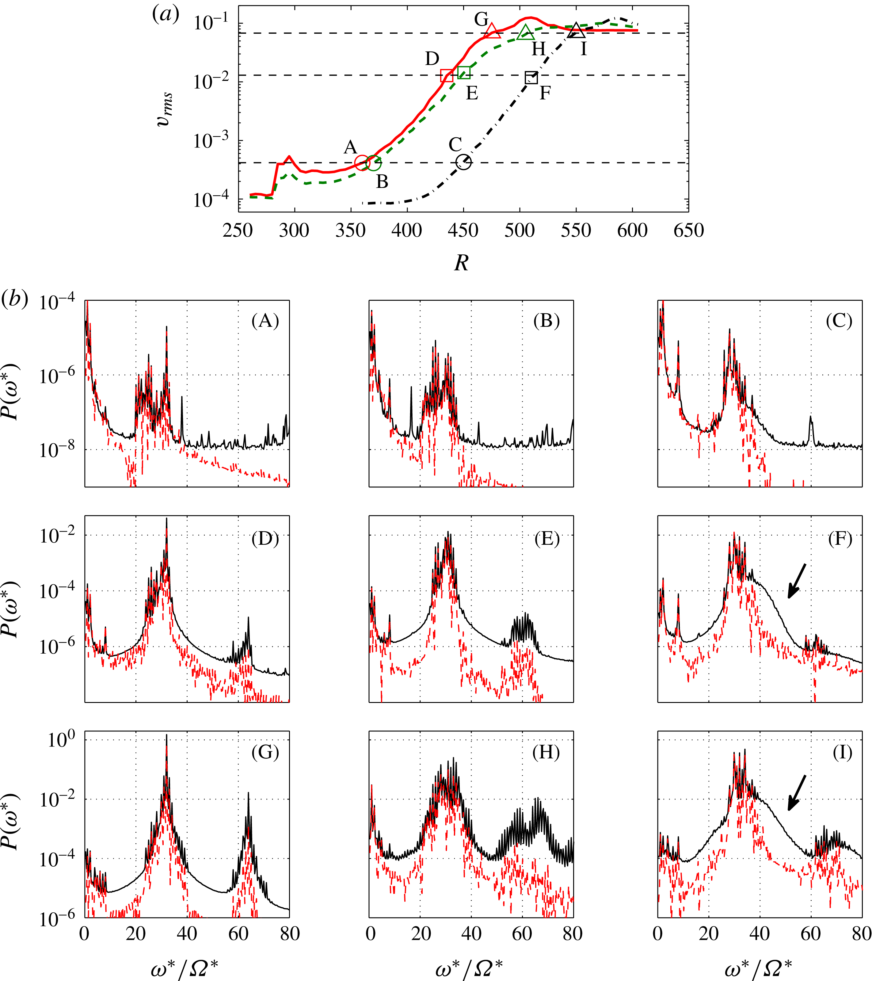
The spectra for cases (D, E, F) are at higher amplitude than (A, B, C). The Reynolds numbers corresponding to (D, E, F) are $R=435$ , 450, 510, respectively. At this amplitude, harmonics of the primary spectral contribution from the stationary vortices are observed at around ${\it\omega}^{\ast }/{\it\Omega}^{\ast }=60$ . This indicates the appearance of nonlinearity. In cases (D, E), the onset of nonlinearity occurs at lower $R$ than the onset of local absolute instability, $R_{CA}=507.3$ , which allows us to attribute the onset of nonlinearity to the growth of Type-I cross-flow instability excited by the surface roughnesses. However, in (F), for the clean disk, a new feature is captured in the spectrum at $R=510$ indicated by the arrow, i.e. a smooth elevated region in the spectrum of the instantaneous time series. This smooth peak was first found in Imayama et al. (Reference Imayama, Alfredsson and Lingwood2014), where it was shown that it is due to a travelling mode rather than a stationary one since it is not captured in the spectra of ensemble-averaged time series. At higher amplitudes, at $R=475,505,550$ , the development of $v_{rms}$ shows a change of slope in figure 11(a), and for cases (G, H, I) the corresponding spectra are shown. The growth of stationary disturbances with $R$ is evidenced by the spiky spectra in (G, H), whereas for the clean disk the growth of both stationary and travelling disturbances is shown in figure 11(b)(I). For case (H), the spectra are very spiky, in particular for the instantaneous time series. This may be caused by the strong asymmetry in roughness (figure 1 b (D)), resulting in asymmetry of the stationary-vortex distribution. Similar results were captured in Siddiqui et al. (Reference Siddiqui, Mukund, Scott and Pier2013). Spectra in their figure 5 showed the onset of nonlinearity before $R_{CA}$ and also spiky peaks at various ${\it\omega}^{\ast }/{\it\Omega}^{\ast }$ similar to case (H).

Figure 12.

Spectra of single-realization (solid line) and ensemble-averaged (dashed line) time series for the clean-disk condition at $R=510$ and (a)  $z=0.6$ , (b)  $z=0.8$ , (c)  $z=1.3$ , (d)  $z=1.6$ , (e) $z=2.0$ , (f)  $z=4.0$ .

To investigate the characteristics of the smooth peak captured in figure 11(b)(F) further, figure 12 shows spectra of single-realization and ensemble-averaged time series measured at $R=510$ at various wall-normal heights. In addition to the spiky peaks, smooth peaks centred on ${\it\omega}^{\ast }/{\it\Omega}^{\ast }\approx 40$ are also observed only in the spectra of single-realization time series. These smooth peaks are more obvious at higher wall-normal positions and are due to travelling disturbances (as they are not shown in spectra of ensemble-averaged time series). Although the observed frequency of about ${\it\omega}^{\ast }/{\it\Omega}^{\ast }\approx 40$ does not fully agree with theoretical prediction of the local absolute instability ( ${\it\omega}^{\ast }/{\it\Omega}^{\ast }=50.3$ at $R_{CA}$ ) by Lingwood (Reference Lingwood1997), Imayama et al. (Reference Imayama, Alfredsson and Lingwood2014) discussed that ‘this perhaps corresponds to the global mode realized in the physical flow, which has a more complex base flow than accounted for in theoretical analyses due, for example, to unavoidable convectively unstable stationary vortices’. The harmonics of these primary peaks are also shown in figure 12, indicating the appearance of nonlinearity, which is highly repeatable for the clean rotating-disk flow. As shown in figures 5 and 6 of Imayama et al. (Reference Imayama, Alfredsson and Lingwood2014), for a clean disk and Reynolds numbers above $R\approx 510$ the nonlinear effects for both stationary and travelling instabilities become dominant and the flow undergoes transition to turbulence.

Imayama et al. (Reference Imayama, Alfredsson and Lingwood2014) showed wall-normal profiles of the unsteady disturbance at several Reynolds numbers in their figure 7. Since the unsteady components contain not only travelling disturbances but also unsteadiness of stationary ones, here, in order to extract purely travelling disturbances from the single-realization time series, bandpass filtering over the range of $40\leqslant {\it\omega}^{\ast }/{\it\Omega}^{\ast }\leqslant 50$ was applied. Figure 12 shows that over this range of frequencies the signal is mainly composed of travelling disturbances.

Figure 13.

Profiles of azimuthal disturbance amplitude from the clean-disk condition. The stationary-disturbance amplitude is obtained by bandpass filtering in the frequency range $31.5<{\it\omega}^{\ast }/{\it\Omega}^{\ast }<32.5$ , whereas the travelling disturbance amplitude is obtained from the frequency range $40<{\it\omega}^{\ast }/{\it\Omega}^{\ast }<50$ . The solid line is the theoretical eigenfunction of the local absolute instability at $R_{CA}$ obtained with parameters from Lingwood (Reference Lingwood1997). The dashed line is the eigenfunction of the local convective instability for stationary disturbances ( $R=507.3$ , ${\it\omega}=0.00447\text{i}$ , ${\it\alpha}=0.268$ and ${\it\beta}=31$ ). The amplitudes are normalized by the maximum disturbance amplitude. (a) ▫, stationary disturbance; ○, travelling disturbance profiles at $R=510$ . (b) Stationary-disturbance profiles at $R=490$ (▵), $R=510$ (♢), $R=530$ (*). (c) Travelling disturbance profiles. The symbols are the same as in (b).

Figure 13(a) shows profiles of stationary and travelling disturbances at $R=510$ from our experiments and eigenfunctions from linear stability theory of the stationary convective instability mode and the critical absolute instability mode. The profiles for the stationary disturbance were filtered in the same way as in figure 8. The profiles in figure 13 are normalized by the maximum amplitude of each profile. The eigenfunction for the stationary mode is calculated with the following parameters: with $R$ and ${\it\beta}$ fixed at 507.3 and 31, respectively, with the real part of ${\it\omega}_{c}$ , which is the angular frequency of the disturbance in the rotating frame, set to zero, and solving temporally for real ${\it\alpha}$ (radial wavenumber) and imaginary ${\it\omega}_{c}$ , giving ${\it\alpha}=0.268$ and ${\it\omega}_{c}=0.00447\text{i}$ . The parameters for the critical absolute instability are given by Lingwood’s (Reference Lingwood1997) table 3. The experimental profile for the stationary disturbances corresponds to the eigenfunction of the stationary mode very closely. Furthermore, the experimental profile for the travelling disturbances is in excellent agreement with the distinct eigenfunction of the critical absolute instability mode. The excellent correspondence between experimental and theoretical results shown in figure 13 indicates that the observed travelling disturbances shown by the smooth peaks in figure 12 are attributable to the absolute instability. This is the first such experimental observation of a global mode directly attributable to the absolute instability of the ‘unexcited’ rotating-disk boundary-layer flow. Figure 13(b,c) shows similar profiles to figure 13(a) but at $R=490$ , 510, 530 together with their respective eigenfunctions. The profiles are normalized by each identified maximum amplitude as in figure 13(a). At each Reynolds number the experimental data adhere nicely to the theoretical eigenfunctions. Although the local absolute instability only exists above $R_{CA}$ , as observed in the numerical study between two rotating disks (i.e. in an open rotating cavity) by Viaud, Serre & Chomaz (Reference Viaud, Serre and Chomaz2008), the global mode is expected to connect smoothly to the upstream convectively unstable region, giving a nonlinear front straddling $R_{CA}$ . Therefore, as expected, the profile of the travelling disturbance at $R=490$ indicates the upstream matching between travelling convectively and absolutely unstable regions.

Figures 12 and 13(a) here, and figure 6 in Imayama et al. (Reference Imayama, Alfredsson and Lingwood2014), show that, for the clean-disk condition, travelling disturbances due to the absolute instability emerge at $R\approx 510$ and the latter paper (Imayama et al. Reference Imayama, Alfredsson and Lingwood2014) shows that the total disturbance field saturates nonlinearly at a well-defined Reynolds number independent of the amplitude of stationary disturbances. This evidence of the influence of a travelling global mode supports Lingwood’s (Reference Lingwood1995) hypothesis that (for a clean disk) the local absolute instability above $R_{CA}$ triggers the onset of nonlinearity and transition to turbulent flow. There is some debate about the route to nonlinearity, i.e. whether that could be via a linear global instability (Healey Reference Healey2010; Appelquist et al. Reference Appelquist, Schlatter, Alfredsson and Lingwood2015) or whether it is via a nonlinear global mode (Pier Reference Pier2003). In either case the global mode would be located by $R_{CA}$ . For example, Huerre & Monkewitz (Reference Huerre and Monkewitz1990) suggested that the global behaviour in spatially developing flows acts as ‘self-excited, low-amplitude wavemaker in the region of local absolute instability’. Pier & Huerre (Reference Pier and Huerre2001) proposed that ‘nonlinear global instability takes place as soon as local absolute instability arises at some point in the flow’ and Pier, Huerre & Chomaz (Reference Pier, Huerre and Chomaz2001) also suggested that ‘the front acts as a wavemaker which sends out nonlinear travelling waves in the downstream direction’, the so-called primary nonlinear steep-fronted global mode (Pier et al. Reference Pier, Huerre, Chomaz and Couairon1998; Pier Reference Pier2003). The present experimental results, the emergence of a travelling global mode and the onset of nonlinearity, align with these theories on front dynamics at the boundary between local convective and absolute instability.

Figure 14.

The disturbance growth and spectral comparisons at a later stage of the transition process. (a)  $v_{rms}$ measured at $z=1.3$ : red solid line, 32 roughnesses [1–32]; green dashed line, 8 roughnesses [1–8]; black chained line, 0 roughnesses (clean-disk condition). $v_{rms}$ labelled by J–R are selected to compare the spectral characteristics of each roughness configuration. (b) Spectra of single-realization (solid line) and ensemble-averaged (dashed line) time series for different roughness configurations: (J, M, P) 32 roughnesses [1–32]; (K, N, Q) 8 roughnesses [1–8]; (L, O, R) 0 roughnesses (clean-disk condition). Labels (J–R) correspond to those in (a).

For comparisons of the later stage of the transition process for the three different roughness configurations, figure 14(a) shows the $v_{rms}$ distributions for the cases of 32, 8 and 0 roughnesses at higher Reynolds number than figure 11(a). At this stage of the transition process, data for the comparisons are selected to give similar points in the transition process rather than for their amplitudes.

Figure 14(b)(J, K, L) corresponds to $R=495,545,570$ , respectively. (J) presents a relatively narrow peak at ${\it\omega}^{\ast }/{\it\Omega}^{\ast }=32$ and the harmonics indicate strong nonlinearity. The spectrum of the instantaneous time series for case (K) shows that energy is distributed across a broad frequency range because breakdown of the stationary vortices excited by eight roughness elements has already occurred, as shown in figure 9(d). However, figure 9(d) also shows that the region that is not influenced by the roughnesses has yet to break down at this Reynolds number ( $R=545$ ). This azimuthal variation in amplitude of stationary disturbances could cause these spiky peaks across the broad frequency range. The spectrum of the instantaneous time series in figure 14(b)(L) for the clean disk perhaps also captures the growth of a smooth part of the spectrum attributed to the global mode, as indicated by the arrow.

The cases (M, N, O) correspond to $R=510,570,585$ , respectively, where the maximum $v_{rms}$ are observed for the three roughness cases. Spectra of instantaneous time series in these figures capture the growth of energy across a broad frequency range, indicating breakdown to turbulence. Finally, (P, Q, R) show the final stage of the laminar–turbulent transition, corresponding to $R=520$ , 590, 600, respectively. It is recognized that the maximum value (excluding peaks at 32 etc.) of $P({\it\omega}^{\ast })$ from the ensemble-averaged time series in (P) is lower than for the two other cases (Q, R), as indicated by the arrow in (P). These low-frequency contributions correspond to the large-scale stationary structures that can appear at breakdown and in the turbulent region of the rotating-disk flow, as discussed in earlier sections of this paper and other papers (Kobayashi et al. Reference Kobayashi, Kohama and Takamadate1980; Corke & Knasiak Reference Corke and Knasiak1998; Imayama et al. Reference Imayama, Alfredsson and Lingwood2014). The main difference between (P) and (Q, R) is the azimuthal variation of the stationary-disturbance amplitude, as shown in figure 9, which, therefore, appears to be important for the growth of these large-scale stationary structures. This finding is not inconsistent with Corke & Knasiak’s (Reference Corke and Knasiak1998) suggestion that resonance between stationary and travelling modes is the trigger.