




No CrossRef data available.
On the Vote-Purchasing Behavior of Incumbent Governments
Published online by Cambridge University Press: 03 March 2004
Abstract
In this paper we investigate whether there are any tactical motives behind the distribution of grants from central to lower-level governments. We use a temporary grant program that is uniquely suitable for testing theories of vote-purchasing behavior of incumbent governments. The temporary grant program differs from traditional intergovernmental grants in several aspects, most importantly in the sovereign decision-making power given to the incumbent central government. We find support for the hypothesis that the incumbent government used the grant program under study to win votes. In particular, we find strong support for the Lindbeck–Weibull/Dixit–Londregan model, in which parties distribute transfers to regions where there are many swing voters. This result is statistically as well as economically significant. We do not, however, find any support for the model that predicts that the incumbent government transfers money to its own supporters.
Information
- Type
- Research Article
- Information
- Copyright
- © 2002 by the American Political Science Association
Are grants from central to lower-level governments tactical, in the sense that the incumbent government uses grants to enhance its reelection probabilities? According to several theoretical models that have evolved in the literature over the past 20 years, this question can be answered positively. Until now, thorough empirical tests of the theoretical models have been lacking, however, since suitable data have been rare. The fact is hence that we do not know whether or not grants are used tactically. It is important, however, to know this, both from a researcher's point of view and from a policy maker's point of view. Since we want to have appropriate models of the political process, researchers need to know whether or not the theoretical models of tactical allocation of grants are valid. A policy maker needs to know whether or not the incumbent government acts tactically when designing grant programs. In this paper, we have access to a data set that is uniquely suitable for use when investigating the vote purchasing behavior of incumbent governments.
In the spring of 1998, a few months before the Swedish elections, 2285 million SEK was distributed to 42 of 115 applying Swedish municipalities. These grants were the first wave of a specially designed support program intended to support, by means of intergovernmental grants, localinvestment programs aimed at an ecological sustainable development and at increasing municipal employment. The decision-making design for these “ecological” grants differs a lot from how the distribution of intergovernmental grants is traditionally performed: The preparation as well as the final decision is made by the incumbent government and there is no explicit formula describing how the grants should be distributed. Furthermore, the grants are not relatedto the efficiency and equity goals otherwise typically attached to intergovernmental grants. Hence, the government has the opportunity to choose freely which municipalities to distribute money to, taking the effect on their reelection possibilities into account.
The purpose of the paper is to use these “ecological grants” to test two competing theories. The prediction from the first model, put forward by Lindbeck and Weibull (1993) and Dixit and Londregan (1996), is that the incumbent government purchases votes by distributing money to regions in which there are many swing voters. In contrast, the prediction from the other model, presented by Cox and McCubbins (1986), is that, due to risk aversion, the incumbent government purchases votes by investing in regions where it already has high support (for example, in regions where the party in power in the local government is the same as the party in power at the central level).
A SUITABLE DATA SET
To test theories that claim that the incumbent central government uses intergovernmental grants for tactical purposes, we would ideally like to have a situation in which (1) the incumbent central government decides on its own whether or not a lower-level government shall be granted, (2) we may disentangle any possible strategic use of grants from the equity and efficiency purposes typically attached to intergovernmental grants, (3) the granting decisions are made in close connection to an election,1
One could argue that, since the money is already distributed, there is no need for voters to reelect the incumbent government and that what ought to matter for voters' decisions is election promises. There is, however, empirical evidence (see, e.g., Stein and Bickers 1994; Levitt and Snyder 1997) that increased spending in fact affects voters' behavior. This could have at least two explanations: One is that voters feel obliged to support those who have treated them well; the other is that voters believe that a party that has supported them in the past also will support them in the future and hence see the actions of the incumbent government before the election as an indicator of how it will act in the future. Whatever the reason is, what matters in the end is that the incumbent government believes that voters react positively if the municipality in which they live is granted. In this paper we assume that this is the case. See also footnote 6.
See, e.g., Bungey, Grossman and Kenyen (1991), Grossman (1994), and Johansson (2002).
Rich (1989) in fact shows that the structure of a grant program, not the specific purpose of the program, shapes the politics of how the grants are distributed. Further, he notes that political factors are more evident in project grant programs than in formula grant programs.
The grant program we study in this paper was introduced in 1997, when it was decided that the Swedish central government should construct a specially designed support program to support, by means of intergovernmental grants, local investment programs aimed at an ecological sustainable development.4
The grant program was initiated by the Committee for an Ecological Sustainable Development.
In 1998, total grants to the municipalities in Sweden amounted to 57.7 billion SEK. Total grants constitute approximately 20% of the municipalities' total revenues. In 1998 1 USD was approximately equal to 8.5 SEK.
There are mainly four aspects that make this data set suitable for the purpose of this paper, besides its economic significance. First, and most importantly, the decision-making process on which of the municipalities are to receive grants differs from the traditional way of distributing grants to municipalities. The usual intergovernmental grants are distributed among the municipalities according to rather strict predefined rules based on equity and efficiency arguments and are handled by central authorities that are independent of the incumbent central government. But for the temporary grants for an ecological sustainable development, it is solely the incumbent central government that decides which municipalities are to be granted (after preparation at the ministry of environment). Furthermore, one of the important decision makers at the Ministry of Environment is a former member of the Swedish parliament for the incumbent government (the Social Democrats). Second, the grant program is not intended to fulfill equity and efficiency objectives but, rather, to “support an ecological sustainable development.” It is, however, far from clear what exactly is meant by that phrase. In fact, there existed no predefined guidelines on how the “ecological” grants were supposed to be distributed (see Riksdagens Revisorer 1999). Third, the decisions were made five to six months before the 1998 elections.6
We can also note that the grant program can be considered a repeated game: it is a four-year program in which the incumbent government distributes money in each of the years 1998–2001. Voters might hence consider the decision made before the election to be an indication of how the incumbent government will act in the future if they win the election (see footnote 1).
The applications for the grants designed for an ecological sustainable development will be made in several waves. We use data from the first wave of applications; hence the analysis in this paper is cross sectional.7
There are at least two reasons for concentrating on the first wave: First, the Swedish Election Survey which we use to estimate one important variable is not yet available for more recent elections; second, the rules for the distribution of ecological grants have been made more structured for the following waves, partly as a consequence of this paper.
TACTICAL REDISTRIBUTION: THEORIES AND EMPIRICAL EVIDENCE
The idea that the incumbent government considers political strengths of regions when distributing resources across the country is old. Investigating New Deal spending, Arrington (1969) found the somewhat mysterious fact that spending did not seem to promote equity between states but rather to favor states with a high income. In fact, economic variables did a very bad job explaining New Deal spending.8
Reading (1973) examines the political rhetoric behind the New Deal. There were three goals of the New Deal: relief, recovery, and reform. He finds no support for the hypothesis that spending and loans were directed to poorer regions, which he takes as evidence that the New Deal did not fulfill the reform goal.
Nevada was the state receiving the largest per capita grants during that period. In addition, Nevada has a 1 in the dummy variable for Senate leadership during the whole period.
Many of the early studies lack a strict theoretical ground and are rather ad hoc about which political variables to include. During recent years, some more stringent theoretical models have been developed. In this paper we concentrate on two competing theoretical models that yield quite different testable empirical implications.10
There are a number of additional hypotheses in the literature, more tailored to the U.S. system, that have been investigated empirically (see, e.g., Stein and Bickers 1994; Levitt and Snyder 1995). Stein and Bickers (1994) investigate the use of pork barrels by incumbent congressmen in the U.S. Congress in the 1988 election. They put forward and find support for the following hypotheses: (i) It is not the dollars spent that matters but, rather, the number of new projects initiated; (ii) not all incumbents need to use grants to improve their electoral fortune—only those in a vulnerable situation (vulnerable meaning that they got elected by a very small margin); (iii) it is not the number of projects per se that makes people like the incumbent but rather, the awareness of these new projects; (iv) awareness increases with the number of new projects; and (v) the electoral support of an incumbent increases with voters' awareness of new projects. Levitt and Snyder (1995) investigate the impact of political parties on federal spending. Underlying the analysis is the assumption that politicians would, if they could, support their own. Levitt and Snyder contrast three models: a “weak party” model, where parties play no role and what matters is whether the representatives of a district have powerful positions in the chamber; a “strong party” model, where parties play a crucial role and where the distribution of outlays changes quickly if the political identity of the district's representatives changes; and an intermediate model, where a party with a sufficiently strong position during a sufficiently long time period is able to favor its own districts. These models are tested empirically by using district-level data on election outcomes and federal assistance programs for the period 1984–1990. Dividing the sample according to geographical concentration, allocation rules, and initiation time, they find that (i) spending is an increasing function of the number of Democratic votes in the district, (ii) spending favors groups that are geographically concentrated being favored, (iii) programs that are allocated through formulas are more heavily skewed to democrats, and (iv) the pattern is strongest for programs initiated during the period 1975–1981, when the Democrats had a strong majority in both the House and the Senate.
The most commonly used theory today is perhaps the one originating from the papers by Lindbeck and Weibull and by Dixit and Londregan. They consider a two-party system where parties, facing an election, promise different groups of voters transfers to win their votes. Voters have preferences over the parties (hereafter ideological preferences) and decide which party to vote for taking these preferences into account, as well as the consumption levels promised by the two parties. In each region there is a distribution of ideological preferences, and given a certain level of regional transfers, there will be a critical value (cutpoint) that divides voters into those voting for one party and those voting for the other party. The parties try to move this cutpoint and thereby increase their vote shares, by using regional transfers.11
More formally, the theoretical model is as follows: Assume that all inhabitants in a region have identical income levels (these are, however, allowed to differ between regions). There are two parties, A and B, maximizing the number of votes. An individual living in region i will vote for party B if U(CiB) − U(CiA) > X, where X is the voter's preference for party A over party B and C is the consumption level promised by party A (when indexed with an A) and party B (when indexed with a B), respectively. The cutpoint in region i is hence defined as Xi = U(CiB) − U(CiA). In each region, there is a distribution of X given by Φi(X), with density φi(X). The vote share for party B is then given by [sum ]i Ni Φi(Xi), where Ni is the share of the population living in region i. Parties maximize their vote shares by choosing Tip, p = A, B (the amount of grants to distribute to each region), subject to [sum ]i Ni Tipk = R, where R is the available resources. At equilibrium both parties choose the same transfer promises, given by the condition UC(Cip)φi(Xi) = UC(CjF)φj(Xj). Grants will hence be an increasing function of the density at the cutpoint [φi(Xi)] and a decreasing function of income (since a higher income means a lower marginal utility of consumption). Since Sweden has proportional election rules, the same results emerge if we assume instead that parties maximize the probability of winning the election. See Dixit and Londregan (1996) for a more detailed description.

The amount of transfers a region receives will hence be positively correlated with the density at the cutpoint. The theory further predicts grants to be targeted at regions with a low income, since voters with a low income have a higher marginal utility of income and thus can be more easily persuaded to vote for a party promising them high transfers than high-income earners can (i.e., the cutpoint moves more in a poor region).12
One main difference between the LW/DL theoretical model and the grant program we study is that the model describes monetary transfers directed directly to individuals, while, in our case, transfers are given to the municipalities to use in investments, which, in the end, affects individual utility positively. It is therefore not obvious how we should expect municipal income to affect the amount of grants the municipality receives.
Note that the closeness proxy is not valid if the distribution functions deviate from the assumptions, for example, if the distribution functions are double-peaked or skewed.
This estimate is obtained using survey data from the Swedish Election Studies. See the Appendix for a description.
The second theory tested is presented by Cox and McCubbins (1986). They divide voters into three groups: support groups, opposition groups, and swing groups. Parties invest in votes by promising redistribution to these groups. Assuming that parties are risk-avert and that swing groups are riskier investments, they predict that politicians will invest little (if at all) in opposition groups, somewhat more in swing groups, and more still in their support groups. It is the assumption of risk aversion together with the assumption that investing in the support groups is the least risky investment which leads Cox and McCubbins to empirical implications different from those of LW/DL. These assumptions can of course be criticized, but they are the ones used by the authors. When testing this model, we use two variables, both assumed to capture the strength of the political support for the incumbent (socialist) government in each municipality. The first is a dummy indicating if there is a socialist majority in the municipal council. The other variable measures the share of inhabitants in each municipality that cast their votes in favor of the incumbent government (the Social Democrats) in the last election.15
It can be noted that an alternative model exists that has been investigated somewhat in the empirical literature, namely, that of Grossman (1994). He takes as a starting point the fact that the same parties appear at both the state and the federal level, and therefore, some interaction between local and central politicians is likely to occur. In the model, federal politicians transfer money to the state level, making it possible for state politicians to raise public spending and thereby increase their reelection possibilities. In return, state politicians invest their political capital in efforts to increase the support of state voters for the federal politicians. The model hence predicts that states where politicians are effective in raising political support will receive large grants from the federal government. The problem, however, is that it is not obvious how to measure political effectiveness, a problem that is illustrated by the fact that the three studies testing this model (Bungey, Grossman and Kenyen 1991; Grossman 1994; Worthington and Dollery 1998) all use different sets of political variables and even predict different signs for some of them. As a consequence of the different views about how political variables influence grants, the empirical evidence is rather hard to interpret. However, the political variables used in these empirical studies closely resemble those implied by the two models discussed in this paper; the closeness of the local elections is very closely correlated with the closeness proxy from the LW/DL model, and two other variables are the same as used by us when testing the Cox–McCubbins model.
Our empirical strategy is as follows. First, we estimate the models developed by LW/DL and Cox–McCubbins separately.16
A difference between the theoretical models and our empirical specification is that the models discuss election promises, made by both parties (blocs), whereas we, in the empirical investigation, investigate actual decisions made by the incumbent government. This means that we are not able say anything about how the opposition bloc would have acted, had it been in the same position as the government. In addition, the theoretical models discuss a situation in which there are only two parties. Sweden, on the other hand, has a multiparty system. However, the political situation has been characterized by the parties divided into two blocs, and this division has been stable over time, meaning that we can consider Sweden a two-bloc system.
For a detailed description on how the variable is constructed, see the Appendix.
The variables used to test the models and their expected signs are summarized in Table 1.

DESCRIPTIVE STATISTICS
Before going into detail about the econometric specifications and the estimation results, we take a quick look at the data here. Is there any pattern that can be observed from data concerning which types of municipalities, on the one hand, apply for grants and, on the other, are granted?
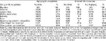
In Table 2 we divide the municipalities into different types depending on their size and population. In the first two columns, we study the applying municipalities, and in the last four columns we study the granted municipalities. From Table 2, we note that all three of the big cities (Stockholm, Malmö, and Göteborg) have applied for grants. Otherwise, the fraction of municipalities applying within each group of municipalities ranges from 30% (for “other smaller municipalities”) to 57.7% (for “larger cities”). Turning to the type of municipalities that was granted, we see that the fraction of municipalities that was granted within each group of municipalities is more unevenly distributed over the different groups of municipalities than is the case for the applying municipalities. From the last four columns in Table 2, it seems that large municipalities (i.e., “big cities,” “larger cities,” and “other larger municipalities”) have been favored, while the opposite seems to be true for “industry,” “rural,” “sparsely populated municipalities,” and “other smaller municipalities.” The most extreme case in the latter group is “sparsely populated municipalities,” where none of the 11 applying municipalities was granted.

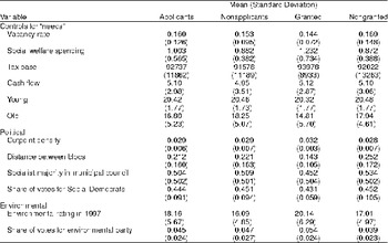
Next we turn to a comparison of the variables used in the empirical analysis. These summary statistics are listed in Table 3. We use the following variables:18
The definitions of the variables are given in the Appendix (under Data Appendix). Summary statistics of the full sample and the raw correlations between the variables are available upon request.
We have also experimented with the unemployment rate instead of the vacancy rate. The unemployment rate, however, had a low explanatory power (in a statistical as well as in an economical sense). In this paper, we report only the results using the vacancy rate.
We have also experimented with other specifications of the rating variable and with survey data, but this does not seem to affect the qualitative results. The survey data used are from the Swedish Election Survey, and from this survey we create variables capturing whether the respondents stated that environmental-related questions are important to them when making their election decisions, the respondents' attitudes to the environmental movement, the importance of a nonpolluting society to the respondents, and, finally, the respondents' worries about pollution.

Starting with a comparison between municipalities applying for grants (applicants) and municipalities not applying for grants (nonapplicants), we note that there are very small differences in the means and standard deviations of the variables. The only variables that seem to differ somewhat are the welfare spending per capita in the municipality and the environmental rating.
Turning to a comparison between granted and nongranted municipalities, we see from the last two columns in Table 3 that several of the variables differ in mean values, notably the political and environmental variables. Starting with the political variables, we note that the granted municipalities are to a lesser extent ruled by a socialist majority (45.2 compared to 53.4%, respectively), a finding that contradicts the prediction derived from the Cox–McCubbins model. The granted municipalities also have a higher estimated cutpoint density (0.032 compared to 0.028) and witnessed closer races between the blocs in the last election (0.143 compared to 0.252 in the election to the central government). These differences are all in line with the predictions derived from the LW/DL model. For the environmental variables, the granted municipalities have a higher environmental rating (20.14 compared to 17.01) and a higher share of votes for the environmental party in the last election to the municipal council (0.054 compared to 0.039). Finally, looking at the “needs” variables, except for the social welfare spending variable, there seem to be no clear differences between the granted and the nongranted municipalities. This fact strengthens our belief that this grant program is free from the equity and efficiency considerations typically attached to traditional intergovernmental grants.
ECONOMETRIC STRATEGY AND EMPIRICAL RESULTS
Econometric Strategy
In the empirical analysis we concentrate on the 115 applying municipalities. That is, we investigate the determinants of whether a municipality receives any grants given that the municipality has applied (that is, in analogy with the program evaluation literature, we investigate the “treatment of the treated”). This is a suitable method to use when trying to determine whether the incumbent government used the specific grant program tactically, which is the main question of interest in this paper.21
If, for some reason, we instead want all municipalities (whether or not they apply) to be the population of interest, we must make sure that the applying municipalities constitute a random sample. If they do not, we will end up with biased estimates. To investigate whether selection matters we have estimated the probit model with selection correction as well. The probit model is given by yi = (β′ xt + ε1i > 0); the selection equation, by yiselect = (γ′ zi + ε2i > 0); and the correlation between the two, by corr(ε1i,ε2i) = ρ [where ε1i,ε2i ≈ N(0,1)]. When selection-correcting the model, we found that (i) we could never reject the null hypothesis that ρ = 0, implying that there seems to be no problems with selection bias, and (ii) the qualitative results were the same as those in Tables 4–6 when we selection-corrected the model.
There are, in principle, two questions that one could be interested in investigating: (i) What determines whether an applying municipality receives grants or not? and (ii) What determines how much the applying municipalities receive? The first question can be investigated by estimating a probit (or logit) model (0/1 variable on the left-hand side, 1 indicating that the municipality was granted and 0 that the municipality's application was rejected) on the 115 municipalities that have applied for grants.22
In this paper we present results obtained with the probit estimator. We have also estimated the model assuming that the error terms are logistically distributed (the logit model). This gave results that were very similar to the probit estimates.
We use a likelihood-ratio test (for a description see Lin and Schmidt 1984). The test statistic, which is distributed as χ2 under the null, is given by λ = −2[lnLT − (ln LP + ln LT)], where LT is the likelihood from the Tobit model and LP and LTR are the likelihoods from a probit model and a truncated regression, respectively. However, since we do not know how well the likelihood-ratio test works in samples of 115 observations and with a rather high degree of censoring (73 of 115, or 63%, of the observations are censored at 0), we have also estimated the models with the Tobit estimator. The qualitative results (in terms of which variables enter significantly and the signs of these variables) in the Tobit model are very similar to those in the probit specification. The Tobit results and the likelihood-ratio tests are available upon request.
In the analysis, we use two sets of regressors. In the first, and most parsimonious, one (Model 1), we use the two variables that are predicted to matter in the LW/DL model (i.e., the municipality's tax base and the political variable) or the Cox–McCubbins model and control only for those variables that are supposed to be important for the grant program under study (i.e., the vacancy rate in the municipality, the municipality's environmental rating in 1997, and the fraction of votes for the environmental party in the last election to the municipal council). In the second one (Model 2), we also control for some different “municipality needs” (i.e., demographic structure, spending on social welfare, and financial result). As argued in the introduction, the setup of the grant program under investigation gives us no reason to suspect these variables to matter. It might, however, be the case that the incumbent government takes equity considerations into account anyway.
Which Municipalities Are Granted? Results of Probit Estimates
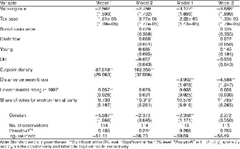
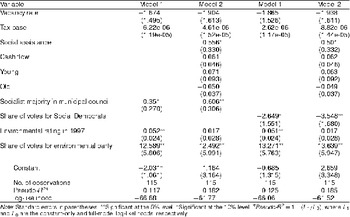
In this section, we investigate the determinants of grant recipience. The probit results are given in Tables 4–6. When testing the LW/DL model, two variables are used to capture the density at the cutpoints: the cutpoint densities and the closeness proxy (i.e., the distance between the political blocs at the central government level).


The results for the LW/DL model are presented in Table 4. From the results in the first two columns, where we use the estimated cutpoint density variable, we note that this political variable is clearly significant in both estimations and has the expected positive sign: the more swing voters there are at the cutpoint, the higher is the probability that a municipality receives money from the incumbent government. This conclusion does not change when we use the closeness proxy instead. From the last two columns in Table 4 we note that this variable, as is the cutpoint density variable, is significant, with the expected sign: the farther apart the two blocs were from each other in the last election (in the election to the central government), the lower is the probability that the municipality will receive any grants. In other words, the closer the race in the last election, the more swing voters there are, and the higher is the probability of getting money from the central government.
Among the other regressors, only the environmental variables and the vacancy rate seem to matter (in a statistical sense), even though none of them enters significantly in all models. Looking at the estimated coefficients, it turns out that the less tight a municipality's labor market (i.e., the lower the vacancy rate) is, the higher is the municipality's environmental rating (in 1997), and the more people there are voting for the environmental party in the municipal election, the higher is the probability that the municipality will get money from the “ecological” grant program. Since all the other control variables are insignificant in all four estimations, it seems that the grant program under study is not used for the equity and/or efficiency purposes that intergovernmental grants traditionally are. We consider the results in Table 4 to lend strong support for the LW/DL model.
Next we turn to the results for the Cox–McCubbins model. We use two political variables, intended to capture the size of the support group, to test this model: “socialist majority in municipal council” (a variable indicating if the party in power in the central government is also in power in the municipal government) and “share of votes for social democrats” (which measures the share of votes in each municipality that the social democrats got in the election to the central government). We see from the results, listed in Table 5, that these political variables have mixed success when it comes to explanatory power. While the variable “socialist majority in municipal council” is insignificant in Model 1 and significant at the 5% level in Model 2, the variable “share of votes for social democrats” is significant in both models: at the 10% significance level in Model 1 and at the 5% level in Model 2. The real problem for the Cox–McCubbins model is, however, that both variables enter negatively in all models, thus contradicting the hypothesis that the government gives money to its own supporters to a larger extent than to supporters of other parties. Among the other regressors, only the two environmental variables enter statistically significantly. Our reading of the results in Table 5 is hence that we do not find any support for the Cox–McCubbins model.
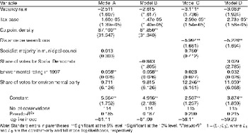
Finally, we turn to the encompassing models to investigate how sensitive the results for the LW/DL model are to the inclusion of other political variables (that is, political variables predicted by the Cox–McCubbins model). The results from the encompassing models are presented in Table 6.24
To save space, we present only the results for the parsimonious Model 1. When the control variables used in Model 2 were included, the political variables from the LW/DL model all entered significantly, with their expected signs, while the political variables from the Cox–McCubbins model were all insignificant.
Given the outcome from this sensitivity analysis, we consider the results for the LW/DL model in Table 4 to be quite robust.
Is the Tactical Use of the “Ecological” Grants of Any Economic Significance?
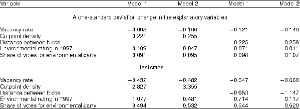
To investigate whether the tactical use of the intergovernmental grants is of any economic importance, we calculate the marginal effects for those variables that were significant in the LW/DL model (Table 4). More specifically, we calculate the change in probability of being granted caused by one-standard deviation changes in the explanatory variables, while the other variables are held at their sample means. In addition, we have calculated the elasticities for these explanatory variables. (These figures are listed in Table 7).

Starting with the results at the top of Table 7, we see that the political variables seem to be economically more important than the labor market and environmental variables; a one-standard deviation increase in the density at the cutpoint or a one-standard deviation decrease in the distance between the blocs yields an increase in the probability that a municipality will be granted with 22–25%. This is to be compared with the corresponding figures for the vacancy rate (which are 10–14%), the environmental rating (1–10%), and for the share of votes for the environmental party (approximately 10%).
Turning to the elasticities in the lower part of Table 7, the same picture emerges. Given model; increasing the density at the cutpoint by 1% or decreasing the distance between the blocs by 1% increases the probability of being granted more than a 1% change in any of the other variables does. This difference is most pronounced for Model 2, where the cutpoint density variable is used, while increasing the density at the cutpoint with 1% increases the probability of being granted with 3.4%, a 1% increase in any of the environmental variables or a 1% decrease in the labor market variable only increases the probability of being granted with approximately 0.5%. When using the distance variable instead, the difference is smaller; a 1% decrease in the distance yields a 0.9% change in the probability of being granted, to be compared with a 0.55–0.7% changes caused by 1% changes in the other variables (Model 1).
CONCLUSIONS
Despite the frequent use of theoretical models describing vote-purchasing behavior of political parties, and despite the common view held by many citizens that the government acts tactically, we have not, until now, been able to investigate empirically whether or not incumbent governments use grants to lower-level government tactically. In this paper a uniquely suitable grant program is used to study the vote-purchasing behavior of incumbent governments. Hence, for the first time we have been able to test theories that have been widely used by economists and political scientist empirically. The findings in this paper are of interest for both researchers and policy makers.
We find support for the hypothesis that the temporary “ecological” grants that we study are used tactically by the incumbent (socialist) government. In particular, we find strong support for the prediction derived from the LW/DL model saying that the incumbent government purchases votes by investing in those municipalities where there are a lot of swing voters. This result is statistically as well as economically significant. The conclusion is strengthened by a sensitivity analysis: It turns out that even though we extend the LW/DL model by political variables predicted by other models, the original variables are unaffected while the added variables enter insignificantly.
We do not find support for the hypothesis that the incumbent government purchases votes by investing in their own supporters (measured as socialist majority in the municipal council and fraction of votes cast for the Social Democrats in the municipality in the last election), a prediction derived from the model presented by Cox and McCubbins (1986).
A resulting question is, of course, Can we generalize our results in some way, or is the formulation of the grant program under study so atypical that no generalizations can be made? It turns out that grant programs similar to the one we study here exist, in Sweden as well as in other countries. It can, for example, be noted that in Sweden, the ecological grants have been followed by other grant programs (for example, to support municipalities that have run into financial problems as a consequence of a balanced-budget law that has recently been put into action) whose allocation principles are very similar to those of the grant program under study in this paper. We can hence expect our results to hold for these other programs as well. At the same time it might be worth stressing that a good way to test the robustness of our results is to investigate how they would fare under other, but similar, grant programs in different countries. If future studies would point in the same direction as ours, we would be more prone to generalize from our results.
Are there any policy implications to be drawn from this study? Well, even though our results strongly indicate that the incumbent government will, if it can, use available resources to win votes, we cannot, from this study, tell whether this leads to a less efficient distribution of grants than if the incumbent did not exhibit any vote-purchasing behavior. However, if one believes that an inefficient distribution of grants is the likely outcome of such behavior, the policy recommendation would be that one should be careful when designing grant programs. In particular, one should avoid programs with vague rules and where the incumbent government has sovereign decision-making power.
APPENDIX
Data Appendix
A description of the variables used in this paper is given below.
Controls for “Needs.”
Vacancy rate: The number of new and remaining vacancies divided by the number of unemployed persons.
Tax base: The municipality's tax base per capita.
Social welfare: Social welfare spending divided by the number of residents in the municipality.
Cash flow: The municipality's cash flow after financial and other costs have been paid.
Young: Share of the population younger than 16.
Old: Share of the population older than 64.
Political Variables.
Cutpoint density: The density at the cutpoint, where the distributions of bias in favor of the opposition are estimated at the constituency level using data from the Swedish Election Studies and the cutpoints are given by the vote share of the winning bloc in the election. See Estimation of the Cutpoint Density, below, for a more detailed description.
Distance between blocs: The difference in vote shares between the socialist and the conservative bloc in the central election, expressed as absolute values. The socialist bloc consists of S, V, and Mp, and the conservative bloc of M, Fp, C, Kd, and NyD.
Socialist majority in municipal council: A dummy taking the value of 1 if S and V have more than 50% of the votes in the municipal council and 0 otherwise.Share of votes for social democrats: The share of votes in each municipality for S in the central government election.
Environmental Variables.
Environmental rating in 1997: The rating is conducted every year by the environmental journal Miljö Eko. The 1997 rating was presented in Miljö Eko No. 5, 1997. The higher the ratio is, the better is the municipality at environmental work.
Share of votes for environmental party: The share of votes in each municipality for Mp in the local government election.
Estimation of the Cutpoint Density
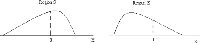
Following Johansson (2002), the variable CUTPOINT DENSITY is estimated using data from the Swedish Election Study of 1994, which is a large survey performed in connection with the election. The data sets are handled and distributed by the Swedish Social Science Data Service (SSD) at Göteborg University. The 1994 study used in this paper was carried out by Mikael Gilljam and Sören Holmberg at the Department of Political Science, Göteborg University. Among the many questions available we picked out variables that we believe capture people's preferences. These variables are listed in Table 8. Respondents are observable at the level of constituency for the parliament. In 1994 there were 29 constituencies. The number of observations in the survey is 2296. These data are then used when estimating the bias in favor of the socialist bloc using factor analysis. All estimations are performed in STATA. The results of the factor analysis estimations are listed in Table 9. When calculating the scores, the regression method is used. Thereafter, constituency-specific distributions of the bias in favor of the socialist bloc are estimated using a univariate kernel density estimator. The bandwidth used is the STATA default, which is the width that would minimize the mean integrated square error if the data were in fact Gaussian and a Gaussian kernel were used. In our case this width is approximately 0.55–0.80. The resulting distributions are given in Fig. 2.


We thank Sören Blomquist, Avinash Dixit, Per Johansson, Henry Ohlsson, and seminar participants at Göteborg University, NTNU, in Trondheim, Stockholm University, Uppsala University, the Research Institute of Industrial Economics (IUI), and the Institute for International Economic Studies (IIES) in Stockholm for helpful comments.
References
Anderson Gary M.
Tollison Robert D.
1991
Congressional Influence and Patterns of New Deal Spending, 1933–1939
Journal of Law and Economics
34
161 75Google Scholar
Arrington Leonard James
1969
The New Deal in the West: A Preliminary Statistical Inquiry.
Pacific Historical Review
38
311 6Google Scholar
Bungey Mel
Philip Grossman
Peter Kenyon
1991
Explaining Intergovernmental Grants: Australian Evidence
Applied Economics
23
659 68Google Scholar
Cox Gary W.
McCubbins Mathew D.
1986
Electoral Politics as a Redistributive Game
Journal of Politics
48
370 89Google Scholar
Dixit Avinash
John Londregan
1996
The Determinants of Success of Special Interests in Redistributive Politics
Journal of Politics
58
1132 55Google Scholar
Dixit Avinash
John Londregan
1998
Ideology, Tactics, and Efficiency in Redistributive Politics
Quarterly Journal of Economics
113
497
529Google Scholar
Grossman Philip J.
1994
A Political Theory of Intergovernmental Grants
Public Choice
78
295
303Google Scholar
Johansson Eva
2002
Intergovernmental Grants as a Tactical Instrument: Empirical Evidence from Swedish Municipalities
Journal of Public Economics
in pressGoogle Scholar
Levitt Steven D.
Snyder James M.
1995
Political Parties and the Distribution of Federal Outlays
American Journal of Political Science
39
958 80Google Scholar
Levitt Steven D.
Snyder James M.
1997
The Impact of Federal Spending on House Election Outcomes
Journal of Political Economy
105
30
53Google Scholar
Lin Tsai-Fen
Peter Schmidt
1984
A Test of the Tobit Specification Against an Alternative Suggested by Cragg
Review of Economics and Statistics
66
174 7Google Scholar
Lindbeck Assar
Jörgen Weibull
1987
Balanced-Budget Redistribution as the Outcome of Political Competition
Public Choice
52
273 97Google Scholar
Lindbeck Assar
Jörgen Weibull
1993
A Model of Political Equilibrium in a Representative Democracy
Journal of Public Economics
51
195
209Google Scholar
Reading Don C.
1973
New Deal Activity and the States
Journal of Economic History
36
792
810Google Scholar
Rich Michael J.
1989
Distributive Politics and the Allocation of Federal Grants
American Political Science Review
83
193
213Google Scholar
Riksdagens Revisorer
1999
Statligt stöd till lokala investerings-program för en ekologiskt hållbar utveckling
[Support to Local Investment Programs Aimed at an Ecological Sustainable Development]
Rapport 1998/1999
8Google Scholar
Stein Robert M.
Bickers Kenneth N.
1994
Congressional Elections and the Pork Barrel
Journal of Politics
56
377 99Google Scholar
Wallis John Joseph
1996
What Determines the Allocation of National Government Grants to the States?
NBER Historical Paper 90Google Scholar
Worthington Andrew C.
Dollery Brian E.
1998
The Political Determination of Intergovernmental Grants in Austria
Public Choice
94
299
315Google Scholar
Wright Gavin
1974
The Political Economy of New Deal Spending: An Econometric Analysis
Review of Economics and Statistics
56
30 8Google Scholar

Variables Used to Test the Different Models and Their Expected Signs
Number of Municipalities Within Each Group that Applied for Grants and that Were Granted
Descriptive Statistics: A Comparison, on One Hand, Between Municipalities Applying for Grants (Applicants) and Municipalities Not Applying for Grants (Nonapplicants) and, on the Other Hand, Between Granted and Nongranted Municipalities
Probit Estimates: Lindbeck–Weibull/Dixit-Londregan Model
Probit Estimates: Cox–McCubbins Model
Probit Estimates: Encompassing Models/Sensitivity Analysis
The Change in the Probability of Being Granted Caused by a one-standard deviation Change in the Explanatory Variables and the Elasticities, for the Lindbeck–Weibull/Dixit–Londregan Model
 You have Access
- 349
- Cited by
Comments
No Comments have been published for this article.