Scholars relying on narrative evidence have described conflicting, but not mutually exclusive, effects of WWII on the demand for labor during and after the war. Some have suggested that the widespread wartime employment of women in industry was a “foot in the door” that opened up new opportunities in predominantly male jobs. The war “may have demonstrated to employers that women could function well in jobs that had previously been male domains,” and it “may have also eroded” policies like marriage bars (Goldin Reference Goldin1991, pp. 742–43). But other historians and contemporary observers have documented numerous examples of women being fired to open up manufacturing jobs for returning veterans.Footnote 1
In this article, we study whether WWII changed the demand for female workers in U.S. manufacturing industries during and beyond the wartime economy. There is already valuable quantitative work on the war and women’s role in the labor force, but that work largely focuses on female labor supply and estimates of wage elasticities of demand without directly measuring the size of the demand change during and after the war relative to 1941, just before U.S. entry into the war as a combatant.Footnote 2 We measure how much the demand (and supply) for different classes of male and female workers—specifically production workers and office workers—changed during and after the war. This is important because the story of increased female employment in the United States around mid-century differs depending on whether it was caused primarily by a shift in demand rather than a shift in supply. Increased labor demand meant better opportunities through higher wages, in contrast with the lower wages associated with an increase in female labor supply.
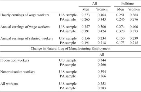
We examine annual data compiled and digitized from industrial surveys carried out by the Pennsylvania Department of Internal Affairs, Bureau of Statistics (various years). This information from Pennsylvania allows us to compare separately the situations for women like “Rosie the Riveter,” who were paid wages on the production line, and women paid salaries in the types of office work in which many had long been employed. The Pennsylvania data also allow comparisons to 1941, which is particularly useful because the economy had nearly recovered to its long-run growth path after a decade of the Great Depression.Footnote 3 Had we used population and manufacturing census data, the latest pre-war year information would be for 1939. Comparisons based on that year would lead to an overstatement of the rise in demand associated with the war because the changes would include part of the recovery from the Great Depression. Finally, if one had to pick a state to study, Pennsylvania would be a reasonable choice because its industry mix most closely matches the nation’s industry mix.Footnote 4 Comparisons of census data in 1939 and 1949 for Pennsylvania and the United States as a whole, reported in Table 1, suggest that the conclusions for the United States as a whole might well be similar if the national-level data for 1941 and the war years were available.
Difference in Natural Log of Earnings of Manufacturing Workers and Change in Natural Log of Employment Between 1939 and 1949 in the United States and Pennsylvania

Notes: Earnings data are calculated from IPUMS Samples for 1940 and 1950 manufacturing workers in manufacturing (variable IND1950 is between 250 and 500) based on annual earnings and weeks worked for the years 1939 and 1949 and number of hours reported worked during the last week of March of 1940. Wage workers are craft workers, operatives, and laborers. Salaried workers are clerks, managers and professionals, and technicians.
Sources: Employment data are from U.S. Bureau of the Census (1957, pp. 45–46).
Our goal is to measure shifts in labor demand (and labor supply), which means measuring the change in quantity demanded (and quantity supplied) while holding earnings constant. Comparisons of means for 1941 and the 1948–1950 period show that the labor demands for both female wage workers and female salaried earners were higher after the war than in 1941. Both earnings and employment after the war were higher than they had been before the war, and the logic of supply and demand implies that this can only happen if demand has increased. More can be said about the size of the shift in labor demand by making assumptions about the elasticity of labor demanded with respect to earnings. Using labor demand elasticities ranging from a highly inelastic −0.3 to an elastic −1.5, the Pennsylvania data imply increases in demand from before U.S. entry into the war to its aftermath of 26 to 40 percent for production wage earners and 44 to 62 percent for salaried workers.
This is only the starting point because we would like to know more about what caused this rise in demand. Was it just a continuation of a long-term trend that would have occurred without the war? How much of a rise in demand for female workers is left unexplained after controlling for changes in wages for other types of workers, unionization, industry mix, educational attainment, and average age?
We address these issues in multiple ways. First, the changes in the 1940s are compared with counterfactual trends between business cycle peaks in 1923 and 1929, a period of relatively rapid growth in the economy, rapid increases in average education for females, and increases in female employment. Over the broad range of demand elasticities, the demand for female production workers rose between 16 and 23 percent faster during the 1940s than during the 1920s, while the demand for female salaried workers rose 17 to 19 percent faster. This type of overall rise in demand occurred across all of the industries studied here.
Second, we then use regression analyses for panels of nine industries for the years 1923 to 1929 and 1941 to 1948 to calculate the residual trends for each type of worker after controlling for changes in wages of the other three types of workers, unionization, ethnic and racial mix in the industry, industry wide productivity changes, and industry mix. The 1940s residual rise in demand for female production workers was more than 58 to 78 percent higher than the 1920s residual rise. However, this residual demand for female salaried workers rose about the same amount in the 1940s as in the 1920s.
Third, using data on earnings in 1939 and 1949 from the IPUMS census microdata samples (Ruggles et al. Reference Ruggles, Genadek and Goeken2015), we perform regression analyses and Oaxaca decompositions of changes in mean earnings for women between the two years (Oaxaca Reference Oaxaca1973). The comparisons show that only a small share of the rise in earnings in the 1940s was associated with increased means for schooling, age, changes in marital status, racial mix, and industry mix. We estimate that the residual change in demand after controlling for all factors we can measure was more than 42 percent for female production workers and very small for female salaried workers.
Comparisons that walk through this same process to calculate the demand for females relative to the demand for males in wage work show the same type of results. Thus, the analysis suggests that there is a large rise in the demand for female production workers between 1941 and the late 1940s that cannot be explained by the factors typically found in wage regressions. Some share of that residual rise is likely associated with women developing skills during the war, adjustments of technology to better match women’s skills, and employers taking more favorable views of the hiring of women in industry once large numbers of women proved their mettle during WWII.
World War II and the Labor Market for Women
When the United States declared war in response to the Pearl Harbor attack in December 1941, its economy had almost fully recovered from the depths of the Great Depression. Female employment in Pennsylvania manufacturing had roughly recovered to its long-run trend level after drops of 20–30 percent between 1929 and 1930. During the war, the United States implemented a quasi-command economy to support the war effort. By 1944, roughly 18 percent of the labor force was serving in the military, and another 22 percent produced output devoted to the war. The military, with limited civilian oversight through the War Industries Board, controlled the allocation of materials necessary for the war (Higgs Reference Higgs1991, pp. 43–44). Large amounts of manufacturing shifted almost entirely from consumer goods to the production of war goods. The large-scale induction of men into the armed forces drew many women into the labor force, in both salaried and production jobs in manufacturing and other sectors (Pidgeon Reference Pidgeon1944). Wage and salary ceilings began in September 1942 and lasted until 1946 (Higgs Reference Higgs1991).
When the war ended in 1945, the demobilization of the armed forces occurred relatively quickly. Once wage controls ended in 1946, labor markets were freed to move toward market equilibria (Higgs Reference Higgs1999). By 1950, the United States was back on a peacetime footing with an unemployment rate of 5.2 percent. Real gross domestic product (GDP) per capita was 29.1 percent higher than in 1941, implying an annual average trend growth rate of 2.9 percent since 1941 (Carter et al. Reference Carter, Gartner and Haines2006, series Ca11, pp. 3–25, 3–26).
The 1970s literature on women’s work and WWII emphasized the war’s transformative effect.Footnote 5 Prior to 1940, women—particularly married women—faced substantial obstacles to paid work: segregation into low-wage occupations, legal constraints on daily and weekly hours, limited access to union membership, personnel policies that barred work for married women, and a workplace ideology dismissive of women (Goldin Reference Goldin1990). The increased demand for labor due to mobilization for WWII and the sharp decline in the number of men available for civilian work pushed the female labor-force participation rate from 32.5 percent in December 1941 to 40 percent in March 1944 (Goldin Reference Goldin1991, p. 748). As the story goes, the disruptive change substantially altered attitudes toward women in the workplace. Alan Clive (Reference Clive1979, pp. 51–52) found that early in the war a number of employers opposed hiring women because they “did not understand machinery and were not trainable.” Further, they complained of the added costs of adjusting machinery and adding restrooms. Once employers began employing women, however, they reported that women had lower-absentee rates, were more motivated, could learn quickly, were better at dealing with intricate components than men, and had aptitude for “dull, repetitive tasks.” Even though Clive suggests that employers’ attitudes reflected a “condescending undertone,” the employers’ attitudes changed enough that women’s opportunities in manufacturing expanded after the war relative to their pre-war situation.
Similarly, numerous Women’s Bureau studies described employer satisfaction with their female workers.Footnote 6 The Women’s Bureau (1947) presented evidence that women’s work during the war altered family roles, for example, with respect to childcare, meal preparation, and other household responsibilities. Raquel Fernandez, Alessandra Fogli, and Claudia Olivetti (Reference Fernandez, Fogli and Olivetti2004) suggest that WWII had lasting effects on women’s labor-force participation by changing the attitudes of sons of working mothers to be more accepting of women at work.
Not all historians have agreed that the war was transformative. Claudia Goldin (Reference Goldin1991, p. 743) reported that the historical literature in the 1980s provided evidence that questioned this narrative, citing D’Ann Campbell’s (Reference Campbell1984, p. 236) conclusion: “It is difficult to argue that World War II, in itself, constituted a watershed in the experience of American women.” Even though many women who joined the workforce during the war sought to remain at work, women were laid off in large numbers as employers and unions gave preference to men in retention and hiring (e.g., see Clive Reference Clive1979; U.S. Women’s Bureau 1948).
The quantitative studies to date mention the possibility that employer demand might have changed as a result of the war, but they do not develop estimates of the magnitude of the demand change associated with the war. The studies do provide valuable information that provides context for the demand changes that we measure in this article. Goldin (Reference Goldin1991) uses individual-level retrospective surveys from Palmer (Reference Palmer1954) to show that the wartime rise in female employment was smaller than the rate of increase of female employment from 1944 to 1950. Many women who were working in 1950 had already been working in 1940, while many others began working after the war. Goldin (Reference Goldin1991, p. 755) suggests that the long-run rise of the clerical sector and in women’s education may have influenced the changing economic role of women more than the war. Meanwhile, some of the increase in labor force participation during the war came from women who had been officially out of the labor force because they were on work relief with the Works Progress Administration (Finegan and Margo Reference Finegan and Margo1994).
Daron Acemoglu, David Autor, and David Lyle (Reference Acemoglu, Autor and Lyle2004) use an instrumental variable analysis of individual-level data from 1939/1940 and 1949/1950 to estimate a female labor supply curve, the wage elasticity of female labor demand, and the impact of female labor supply on the female/male earnings differential. Assuming a constant elasticity of substitution production function, they find that women in states with greater mobilization of men during WWII worked more after the war in 1950 even though they did not work more in 1940. Following similar procedures, Goldin and Olivetti (Reference Goldin and Olivetti2013) find that employment gains were concentrated among women with at least a high school degree. Moreover, women with no children during WWII were the ones most affected by manpower mobilization in 1950.
Estimating the Size of Shifts in Supply and Demand with Information on Earnings and Employment
As a starting point, we can draw simple conclusions about the relative size of shifts in labor demand and supply by assuming a downward sloping demand and upward sloping supply and then comparing the change in earnings and employment. For example, if we see that earnings and employment rise, we can infer that a rise in demand dominated all other shifts.
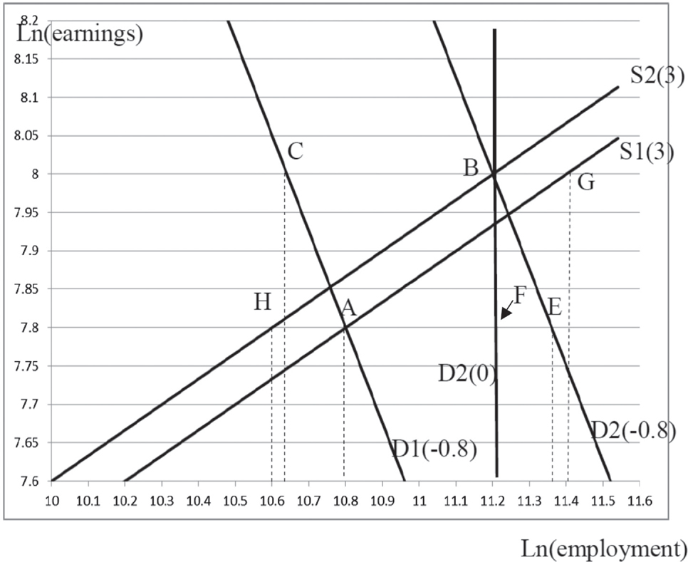
The analysis can be more specific about the size of changes in labor demand and supply by making assumptions about the elasticities of employment (E) with respect to earnings (W) for the labor demand and labor supply curves. Consider the log linear demand and supply functions plotted in Figure 1. To make the discussion easier to follow and illustrate the actual change from before the war to after the war, we chose measures of ln(earnings) and ln(employment) that roughly correspond with the values observed for 1941 and 1949/1950 in Table 2 for female salaried workers. The starting equilibrium is point A, where demand line D1(–0.8) intersects with supply line S1(3), ln(earnings) equal 7.8, and ln(employment) is 10.8. The values in parentheses for D1 and S1 are the assumed elasticities of employment with respect to earnings used to draw the supply and demand lines. After demand rises to D2(–0.8) and supply falls to S2(3), the new equilibrium is at point B, where ln(earnings) equal 8 and ln(employment) is 11.2.
Measuring the Size of Demand and Supply Shifts in Different Ways and with Different Elasticities

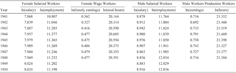
The Natural Logs of Average Real Annual Salaries and Employment for Male and Female Salaried Workers and of Real Average Hourly Earnings and Total Hours Worked by Male and Female Wage Workers in Pennsylvania, 1941 to 1950

Sources: Pennsylvania Department of Internal Affairs (various years between 1941 and 1950), Beney (Reference Beney1938), and NICB (various months between 1941 and 1948). Average earnings and salaries are adjusted for inflation using the Consumer Price Index with 1967 = 1 (U.S. Census Bureau 1975, series E-135, p. 210).
The size of the demand change is defined as the horizontal difference in ln(employment) between points on the new demand curve and the old demand curve measured at a specific level of ln(earnings). In practice, the measurement is either made at the original ln(earnings) of 7.8 or the new ln(earnings) of 8. The actual change in ln(employment) that occurs in Figure 1 is a rise of 0.4 from 10.8 at point A to 11.2 at point B. To find the change in ln(employment) caused by the demand shift, we need to subtract the change in ln(employment) associated with the change in ln(earnings) from the actual change in ln(employment) between points A and B. The equation takes the form:
 $\rm{DD} = [\ln ({E_B}) - \ln ({E_A})] - {e_D}[\ln ({W_B}) - \ln ({W_A})].$
DD is the demand shift measure, EB and EA are employment at locations A and B, WA and WB are earnings at points A and B, and eD is the demand elasticity of employment with respect to earnings, which is assumed to be negative. Thus, the shift measure can be rewritten using the absolute value of the demand elasticity |eD| as
 $\rm{DD} = [\ln ({\rm{E}_\rm{B}}) - \ln ({\rm{E}_\rm{A}})] + \left| {{\rm{e}_\rm{D}}} \right|[\ln ({\rm{W}_\rm{B}}) - \ln ({\rm{W}_\rm{A}})].$
A mathematical derivation of the equation is shown in Online Appendix 1.
To see the change in demand associated with this change in equilibrium in Figure 1, pick a level of ln(earnings) and then measure the gap between ln(employment) at that level. Pick ln(earnings) of 8 at the new equilibrium B, and the gap to be measured is the horizontal difference between points B and C of 0.56 (=11.2–10.64). From equation (1) that difference is: the observed change in ln(employment) of 0.4 (=11.2–10.8) from moving from equilibrium A to B minus the drop in ln(employment) of −0.16 (=10.64–10.8) between points A and C. The change in ln(employment) from A to C is the reduction in ln(employment) of −0.16 along the original demand D1(–0.8) caused by the observed 0.2 rise in ln(earnings) from 7.8 to 8. This −0.16 reduction is the change in ln(earnings) of 0.2 multiplied by the elasticity of −0.8. The demand change also can be measured at the original ln(earnings) of 7.8 as the horizontal difference between points A and E.
Notice that the labor supply elasticity does not play a role in measuring the size of the demand shift because the demand shift is measured as the horizontal change in ln(employment) between points on the two demand curves at the same ln(earnings) level. The labor supply elasticity plays only an indirect role as one of the determinants of the location of the observed equilibrium points A and B in Figure 1. The observed change in ln(employment) establishes that horizontal difference between A and B, so we do not need the labor supply elasticity to find it. Once we know the horizontal difference between A and B, the horizontal difference associated with the demand shift is found by exclusively using the labor demand elasticity of employment with respect to earnings.
Equation (2a) shows that the measurement of the demand shift differs with the elasticity assumed. If we assume a perfectly inelastic new demand D(0) with an elasticity of 0, the demand line would be the vertical line D2(0) at ln(employment) of 11.2. We are still comparing equilibriums at points A and B because D2(0) passes through the new equilibrium at point B. When the demand shift is measured at the original ln(earnings) of 7.8, it is the horizontal gap between A and F. The elasticity of 0 for D2(0) implies no change in ln(employment) associated with the rise in price that leads to the new equilibrium at point B. As a result, the horizontal gap between A and F is the same as the horizontal gap between A and B and equals 0.4. The demand shift with this more inelastic demand is smaller than when we had a more elastic demand elasticity of −0.8. In general, when both ln(earnings) and ln(employment) rise, a more elastic demand assumption will lead to a larger measured rise in demand.
There is one other feature to note here. When the equilibrium moves from point A to point B and we measure the demand change, we are always making an assumption about the elasticity of only one of the demand curves. Thus, if the elasticity of the original and the new demand curves are different, we will get different estimates of the demand shift depending on which elasticity is used; therefore, it is important to provide a range of estimates of the demand shift if it is probable that the demand elasticity had changed.Footnote 7
The measurement of a supply shift follows a similar process. The supply shift SS is calculated as the actual change in ln(employment) minus the change in ln(employment) that arises from multiplying the supply elasticity eS by the change in earnings between the two equilibrium points.
 $\rm{SS} = [\rm{Ln}(\rm{E}) - \rm{Ln}(\rm{E}^*)] - {\rm{e}_\rm{S}}[\rm{Ln}(\rm{w}) - \ln (\rm{w}^*)]$
On Figure 1, the measure of the supply shift from S1(3) to S2(3) when using the new ln(earnings) of 8 is the horizontal distance of −0.2 (=11.2–11.4) between points G and B. We observe ln(employment) of 10.8 at A and 11.2 at B. Finding point G requires an assumption about the supply elasticity of ln(employment) with respect to ln(earnings). S1(3) assumes a supply elasticity of 3. The 0.2 rise in ln(earnings) between points A and B would have led to a rise in ln(employment) along S1(3) from 10.8 at A to 11.4 at G. The difference of 0.6 can be found by multiplying the rise in ln(earnings) of 0.2 by the supply elasticity of 3. Using equation (2b), the measure of the change in supply is −0.2, which is the actual change in ln(employment) from point A to B of 0.4 minus the change in employment from A to G associated with the ln(earnings) rise) of 0.6.
If we were to measure the supply change at the original ln(earnings) of 7.8 the supply reduction would be measured as the horizontal reduction between points A and H, which would be the actual gap in ln(employment) between A and B of 0.4 minus the estimated gap in ln(employment) between B and H of 0.6 along the new supply curve S2(3). If the elasticity is assumed to be 3, the reduction in supply will again be −0.2.
The measurement of supply and demand shifts moving into and out of WWII is complicated by the wage and salary ceilings imposed by the federal government between September 1942 and 1946. In Online Appendix 2 we show that the presence of a wage ceiling will not cause problems for estimating shifts in labor supply using comparisons of actual ln(earnings) and ln(employment). However, the true size of the demand increase during the war is understated and the fall in demand between the war era and the post-war era is also understated.
Measuring the Effect of the War by Comparing to a Counterfactual Trend
The demand and supply shifts measured above are the raw changes during the war. They describe the impact of the war if we believe that the situation would have stayed the same as in 1941 without the war. Goldin (Reference Goldin1990), however, notes that there were substantial changes in women’s roles in the 1920s and 1930s that likely would have continued had the war not been fought. We therefore develop a counterfactual trend set of predictions of what would have happened had the war not been fought. Because the demand and supply shift equations are log linear, we can calculate the size of the actual demand shift relative to the counterfactual shift (ΔDD) by subtracting the counterfactual change (subscript C) from the actual change (subscript A). A similar calculation can be made for the relative change in supply (ΔSS).
 $\Delta \rm{DD} = [\Delta \ln ({\rm{E}_\rm{A}}) - \Delta \ln ({\rm{E}_\rm{C}})] + \left| {{\rm{e}_\rm{D}}} \right|[\Delta \ln ({\rm{W}_\rm{A}}) - \Delta \ln ({\rm{W}_\rm{C}})]$
 $\Delta \rm{SS} = [\Delta \ln ({\rm{E}_\rm{A}}) - \Delta \ln ({\rm{E}_\rm{C}})] - {\rm{e}_\rm{S}}[\Delta \ln ({\rm{W}_\rm{A}}) - \Delta \ln ({\rm{W}_\rm{C}})]$
Δln(EA) is the actual and Δln(EC) is the counterfactual change in ln(employment), and Δln(WA) and Δln(WC) are the actual and counterfactual changes in ln(earnings). This difference provides a more likely estimate of the change in demand directly related to the war experience by subtracting out changes that likely would have occurred without the war.
The counterfactual trend in Pennsylvania is based on the average annual growth in earnings and amount of labor between 1923 and 1929 for several reasons. This was the only extended non-crisis period for which data are available on a consistent basis prior to 1950. The years 1923 to 1929 were both business cycle peaks during the only non-crisis period for which data are available before 1950. These were boom years for the economy with minor fluctuations. There was substantial growth in new technologies like automobiles, radios, and electricity, a rise in leisure activity, expansions in internal labor markets, increases in the access to high school and more advanced education, and changed political roles for women after they obtained the right to vote. The period 1923 to 1929 also led to expansions in labor market activity by Pennsylvania women. The average annual growth rate in the number of female salaried employees was 2.45 percent per year and their real salaries grew at 1.6 percent per year. Meanwhile, employment of female wage workers rose 1.4 percent per year and their real average annual earnings rose 1 percent per year.Footnote 8
The Importance and Choice of Labor Demand and Supply Elasticities
In a number of situations we can learn a great deal about the change in demand and supply from just looking at changes in ln(employment) and ln(earnings) without choosing specific demand and supply elasticities. For example, if there is no change in ln(earnings), substitute zero for the change in ln(earnings) in equations (2a) and (2b) and the change in labor demand and labor supply is equal to the change in ln(employment). In the analysis below, the changes in ln(earnings) after subtracting the counterfactual for female salaried workers are small enough that the size of the demand change is mostly determined by the change in counterfactual adjusted ln(employment).
If both ln(employment) and ln(earnings) rise, the demand clearly rises by at least the rise in ln(employment) and is amplified more by the rise in ln(earnings) when labor demand is more elastic.Footnote 9 These types of situations adjusted for the counterfactual occur for female wage workers in the analysis below, so that we get a clear picture of the direction of the changes in demand and a good sense of the magnitude of the change for female workers no matter which elasticity is assumed.
On the supply side, the negative sign in front of the supply elasticity implies that when ln(employment) rises and ln(earnings) fall, supply definitely rises by at least the change in ln(employment), and the size of the supply rise is amplified when a larger supply elasticity interacts with the decline in wages. In the analysis below this setting is common for male production and male salaried workers. The increases in ln(employment) are large enough that we know there was at least a large rise in male labor supply, although the full size of the rise varies a great deal across the range of supply elasticities reported in the literature.
There are two situations in the analysis below in which the elasticity assumption becomes a major determining factor. The first happens when ln(employment) and ln(earnings) move in opposite directions when trying to measure a demand shift. This is the situation for male salaried and male production workers. The literature on estimating demand elasticities shows a range from close to zero to around −1.5 for various estimates of demand elasticities. We found only one estimate that was specific to manufacturing workers. Richard Freeman (Reference Freeman1980, pp. 7, 18–19) estimated long-run manufacturing labor demand elasticities of −0.33 to −0.6 using time series analysis with lagged values as instruments. Daniel Hamermesh’s (Reference Hamermesh1993, pp. 270–73) summary of demand elasticities for all males suggests that the demand is generally inelastic and the estimates range from zero to minus one. Acemoglu, Autor, and Lyle (Reference Acemoglu, Autor and Lyle2004) estimate that the demand elasticity for all women workers was more elastic and ranged between −1 and −1.5. Given our focus on manufacturing, which had more specific skill requirements than general labor demands, employers would have had fewer substitute workers from which to choose, making the manufacturing labor demand more inelastic than the demand for all workers as a category. Our best guess of the manufacturing labor demand elasticity is that it was in the −0.5 to the −1.0 range for production workers. Yet, there remains a great deal of uncertainty about the right elasticity to choose for each type of worker, particularly because we are also looking at salaried workers of both genders as well. As a result, we report labor demand changes for elasticities of −0.3 to −0.8 to −1.5 to cover the ranges we have seen in the literature.
A second setting where the choice of elasticity is important occurs when ln(employment) and ln(earnings) move in the same direction when trying to measure a supply shift, as happens below for female production workers.Footnote 10 The range of labor supply elasticities in the literature is much larger and there is a substantial debate (Keane and Rogerson Reference Keane and Rogerson2012; Chetty et al. Reference Chetty, Guren and Manoli2011). Part of the debate centers on differences in the level of aggregation in estimation. Studies of individual data often find small elasticities that are well below one, while macroeconomists focusing on aggregate data for the whole labor force use elasticities ranging from one to three. Michael Keane and Richard Rogerson (Reference Keane and Rogerson2012) argue that the small estimates from individual data imply the larger elasticities with aggregate data, but Chetty et al. (Reference Chetty, Guren and Manoli2011) still argue for aggregate elasticities below one. Neither the individual nor the macro elasticities exactly fit the context we are examining because the macro estimates are for the entire economy and the micro estimates are for individuals. The one set of estimates we found specific to manufacturing was Freeman’s (Reference Freeman1980) long-run estimates in the 5–6 range using time series analysis with lagged values as instrumental variables. The larger elasticity for manufacturing as opposed to all types of work makes sense because workers have more options outside of manufacturing. Based on intuition and our use of aggregated hours and employment and mean earnings, we expect the elasticity in the Pennsylvania setting to be in the 3 to 5 range. Here again, we provide a broad range of estimates for the reader to show the results for the broad range in the literature.
Data
To obtain information on earnings and employment, we joined Ryan Johnson (Reference Johnson2002) in compiling a gender-specific industry-level data set from reports of various titles from annual surveys by the Pennsylvania Department of Internal Affairs, Bureau of Statistics (various years between 1915 and 1950). The Bureau annually sent out a team of field workers who conducted surveys and also kept in close contact with Chambers of Commerce to ensure that the department collected data on all relevant firms (Pennsylvania Department of Internal Affairs 1941, p. xvi). The data were collected annually and span the years 1916 to 1950 for more than 300 industries in Pennsylvania. We aggregated the industries into nine categories to eliminate problems with plant information being reported in one subcategory in one year and another category in other years (Shatnawi Reference Shatnawi2010). Comparisons with data by industry for Pennsylvania from other sources showed high correlations in the overlapping years from the sources.Footnote 11 The complete dataset is available for download from Open ICPSR (Fishback and Shatnawi Reference Fishback2018).
The reports provided information on the number of workers and total payments to the workers for four categories: male wage earners, female wage earners, male salaried workers, and female salaried workers. Later in the article we will also incorporate information on the value of the product, share of black workers, and share of foreign-born workers from the Pennsylvania reports.
Given the nature of wage payments for salaried workers, who were not paid by the hour, the average salary is a good estimate of the wage that workers consider when choosing between firms. For production workers, who were typically paid by the hour or the piece, the annual earnings are influenced by hours worked, which are a component of the labor supply. Therefore, we obtained measures for male and female production workers of hourly earnings and average hours per week in 25 industry classifications between 1920 and 1948 from the National Industrial Conference Board (NICB).Footnote 12 The data were collected from the NICB monthly reports titled Personnel Management Record for the years between 1939 and 1950.Footnote 13 We digitized the same information for the years 1920–1936 from Ada Beney (Reference Beney1938) who also collected them from the same source. The data were reported monthly, and we convert the monthly averages into annual averages so that we can match and merge the national wages to the annual Pennsylvania data. The NICB data cover the entire country, but Pennsylvania accounted for 13 percent of the firms surveyed (NICB 1930, pp. 34–35). We have looked at other sources of hourly earnings and hours worked by state for the years 1933, 1935, 1937, and 1939 and for later years, and Pennsylvania’s hourly earnings track reasonably closely to the national hourly earnings over time in those sources.
As described earlier, the Pennsylvania data offer some advantages over the population and manufacturing census data available in 1939 and 1949. First, and most importantly, the availability of annual data allows better comparisons to the pre-war but post-Depression situations for men and women. While 1939 was still a Depression year, the economy had nearly recovered to its long-term trend path in 1941. The average annual growth rate in real GDP per capita between 1929 and 1941 was 1.5 percent per year, similar to the long-term trend of 1.6 percent for the past 160 years. The number employed as a share of the population had reached 37.7 percent, 0.3 percent lower than in 1929 and the unemployment rate was 9.9 percent if relief workers are considered unemployed. If relief workers are considered employed, employment as a share of the population had reached 39.4 percent, 1.4 percent above the pre-Depression peak in 1929, and the unemployment rate had fallen to 6 percent.Footnote 14 When choosing years after the war for comparisons, we do not push past 1950, so we can avoid the military expansion and limits on markets associated with the Korean War. Second, we can calculate peacetime counterfactuals from the 1920s using data that were collected in the same way. Third, the Pennsylvania data provide detailed information on female wage workers, female salary workers, male wage earners, and male salary earners that is not available in the manufacturing census reports.
As mentioned in the Introduction, the situation in Pennsylvania manufacturing in the 1940s is likely to have been similar to the situation for U.S. manufacturing as a whole. Pennsylvania’s manufacturing was broad based, and its distribution of industries was more closely matched to the U.S. national distribution than the distribution in any other state. Even though we prefer not to use 1939 as a pre-war year in the baseline analysis, we can make comparisons of the changes between 1939 and 1949 in ln(earnings) and ln(employment) for Pennsylvania and the United States using data from the manufacturing and population censuses in Table 1. The changes differ somewhat between Pennsylvania and the United States, but the differences are small enough that the qualitative findings for changes in labor demand in Pennsylvania may offer a useful estimate of what was happening in U.S. manufacturing as a whole.
Demand and Supply Shifts in the Actual Data and Relative to the Counterfactual
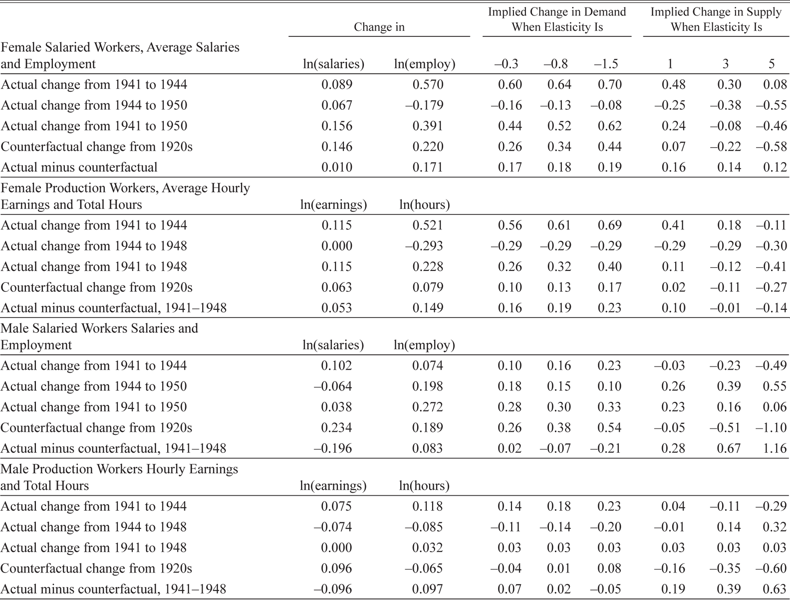
Table 2 shows the information on the natural logs (ln) of real average annual salaries and average employment that we use to calculate the actual shifts in demand and supply for the period 1941 through 1950. The shift calculations in Table 3 show the size of the demand shifts associated with these changes over a broad range of demand elasticities of employment (or hours) with respect to earnings of −0.3, −0.8, and −1.5. The supply shifts are shown for elasticities ranging from one to five. In the discussion we focus on a labor supply elasticity of 3 and a demand elasticity of −0.8 to simplify the exposition.
Sizes of Actual Demand and Supply Shifts for Female and Male Salaried and Wage Workers During and After the War and Shifts Relative to the Counterfactual, 1941–1950
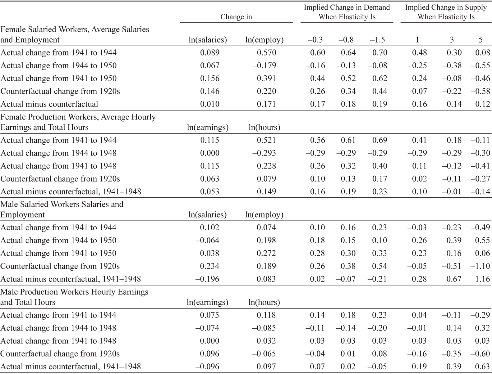
Notes: The 1940s measures in the first two columns are calculated using information in Table 2. The implied changes in demand and supply are based on equations (2a) and (2b). The changes relative to the counterfactual are based on equations (3a) and (3b). The counterfactual is based on the changes between 1923 and 1929 and then adjusted to match the length of time for comparisons with the 1940s data. The change in demand is measured as the change in ln(employment) (or ln(hours)) between the original demand and the new demand, holding ln(earnings) constant. The definition is similar for the measure of the change in supply.
Sources: See data section in the text.
Female Salaried Workers
Female salaried workers were typically clerks, administrative assistants, and administrators during the 1940s. Women had been in many of these positions in the 1920s and 1930s even in industries where they were not working on production lines. Between 1941 and the peak of the war effort in 1944, ln(salaries) for female salaried workers grew by 0.089 log points and ln(employment) boomed by 0.57 log points.Footnote 15 These changes imply a rise in demand of 0.641 log points if there had been no salary controls. This is an understatement of the true rise in demand because the salary controls in place after September 1942 prevented the full effects of the demand rise on salaries and employment from occurring. The estimate of the labor supply shift is not affected by the wage and salary controls. At our baseline supply elasticity of 3, the supply shift was 0.30 log points, although it was much smaller at 0.08 log points with an elasticity of 5.
Demobilization began with the end of the war in 1945, and the wage ceilings were removed in 1946. Between the war peak in 1944 and 1950, employment declined and real salaries increased each year except 1946. By 1950, ln(employment) had fallen by −0.179 log points, and ln(salaries) had risen by 0.067 ln(points). The changes imply a drop in demand by −0.13 log points or more because the salary controls prevented us from measuring the full rise in demand to 1944. This drop in demand matches the narratives of layoffs for female workers after the war and the replacement of female workers by the returning male workers in manufacturing. The changes also imply a drop in supply of −0.38 log points from the wartime peak.
Despite the sharp drop-offs in employment after the war, the ln(employment) for female salaried workers in 1950 was 0.391 log points above the level seen in the recovered economy of 1941, while ln(salary) was 0.156 log points above. This implies a large demand rise between 1941 and 1950 of 0.52 log points and a much smaller supply fall of −0.08 log points.
Since the long-run path in the United States has been one of growth and change, it is important to go beyond just comparing the actual situations in 1941 and 1950. We therefore compare the changes to the counterfactual path based on the average annual growth rates in earnings and employment between the two business cycle peaks of 1923 and 1929. The counterfactual trend paths for the natural logs of employment and average salaries start with the actual values in 1941 and then allow each series to grow at the annual trend pace between 1923 and 1929. During that period, real salaries grew at an average annual pace of 0.016 log points per year, and female salaried employment grew 0.024 log points per year. If they had grown at the same pace between 1941 and 1950, ln(employment) would have been 0.22 log points higher and ln(salaries) would have been 0.146 log points higher in 1950 than in 1941. These changes imply a counterfactual demand rise of 0.34 log points and a supply reduction of −0.22 log points.
The differences between the actual 1941–1950 changes and the 1920s counterfactual changes give a better estimate of the impact of WWII on the demand and supply. Table 3 shows that the actual change in ln(salary) between 1941 and 1950 was 0.010 log points higher than the counterfactual change, while the actual change in ln(employment) exceeded the counterfactual change by 0.171 log points. This implies that labor demand rose more than the counterfactual demand by 0.18 log points and labor supply rose more than counterfactual labor supply by 0.14 log points. These differences between the actual and counterfactual demand shifts are robust to a broad range of assumptions about the elasticities.
Female Wage Workers
Between 1941 and the wartime peak in 1944, ln(hours) for female wage earners exploded by 0.521 log points, while the wage controls held the rise in ln(hourly earnings) to 0.115 log points. Had this been a situation with no wage controls, the rise in demand would have been more than 0.61 log points. Meanwhile, female labor supply rose by 0.18 log points, although it should be noted that a supply elasticity of 5 implies a decline in labor supply in Table 3 by −0.11 log points.
Both the demand and the supply for female production workers declined after the wartime peak. Between 1944 and 1948, ln(total hours) declined by −0.293 log points, while ln(hourly earnings) remained virtually the same.Footnote 16 This combination implies a reduction in both demand and supply by around −0.29 log points.
Comparisons of the pre- and post-war settings shows that ln(total hours) rose by 0.228 log points between 1941 and 1948 and ln(hourly earnings) rose by 0.115 log points. These changes imply an increase in labor demand by 0.32 log points and a reduction in supply by −0.12 log points. After subtracting counterfactual changes in employment and earnings based on the 1920s from the actual changes, the labor supply of women between 1941 and 1950 fell barely at all with a supply elasticity of 3, but the direction of the supply shift varies from a rise of 0.1 to a fall of −0.14 over the span of supply elasticities.
The most striking feature of the counterfactual comparisons is the large rise in the demand for female production workers. The demand rose by 0.19 log points more than the counterfactual at an elasticity of −0.8 and by 0.16 to 0.23 log points over the entire ranges of assumed elasticities.
Male Workers
A common belief is that the war mobilization expanded the demand for male production workers just as labor supply fell because large numbers of men were drawn into the military. After the war, the demand for male workers fell back some, while the supply expanded again. The comparisons reported in Table 3 show that the raw changes are consistent with this narrative for both male salaried and wage workers. For male salaried workers, the raw numbers show a rise in salaries and employment from 1941 to 1950, consistent with a rise in demand and a rise in supply during the 1940s. After adjusting for the counterfactual, however, the change in demand was lower and the supply rise was higher than the counterfactual without the war. For male production workers, the raw changes from 1941 to 1948 show very small changes in the 1940s for earnings, time worked, supply and demand. When compared with the counterfactual, there was very little change in the demand for male production workers, but a relative increase in supply.
Changes in Demand for Females Relative to Males
If the elasticities of demand and supply were the same for male and female workers, we could carry the analysis above further to make comparisons of the changes for females relative to males and then comparisons of how females fared relative to males relative to the counterfactual. But it is unlikely the elasticities were the same.
The demands for males and females were connected by the degree to which they were substitutes for each other in the work process. Acemoglu, Autor, and Lyle (Reference Acemoglu, Autor and Lyle2004) and Goldin and Lawrence Katz (Reference Goldin and Katz2008) have derived relative demand functions for different classes of workers based on the elasticity of substitution between the classes of workers. Following Goldin and Katz (Reference Goldin and Katz2008, p. 297) we can write the female/male relative demand function (DFM) as
 ${\rm{D}_{\rm{FM}}} = [[\ln ({\rm{E}_{50}}^\rm{F}) - \ln ({\rm{E}_{41}}^\rm{F})] - [\ln ({\rm{E}_{50}}^\rm{M}) - \ln ({\rm{E}_{41}}^\rm{M})]] + {\sigma _{\rm{FM}}}[[\ln ({\rm{W}_{50}}^\rm{F}) - \ln ({\rm{W}_{41}}^\rm{F})] - [\ln ({\rm{W}_{50}}^\rm{M}) - \ln ({\rm{W}_{41}}^\rm{M})]],$
where the F and M subscripts refer to females and males, the 50 and 41 subscripts refer to the years 1950 and 1941 (1948 and 1941 for production workers), E is employment (or hours), W is earnings, and σFM is the elasticity of substitution in production between females and males. In their analysis, they assumed the supply elasticity was zero in the short run, which implies that the relative supply shift is equal to the difference between the change in ln(employment) for females and males.Footnote 17 Acemoglu, Autor, and Lyle (Reference Acemoglu, Autor and Lyle2004) estimated an elasticity of substitution between male and female labor (σFM) that ranged from 2.4 to 4.2 for all types of labor. We provide estimates for a larger range from 0 to 4 to show the robustness of the relative demand estimates to the elasticity assumptions.
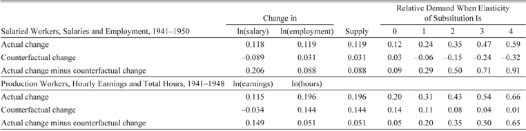
The comparisons in Table 4 show the actual and counterfactual female/male relative changes in ln(earnings) and ln(labor) between the pre- and post-war periods. The supply changes document that female labor increased relative to male labor using the actual numbers and relative to the counterfactual by 0.088 log points for salaried workers and 0.051 points for production workers.
Changes in Relative Female/Male Demand and Supply for Salaried and Wage Workers

Notes: Changes in relative demand were calculated using equation (4). The change in relative supply in this situation is the same as the change in ln(employment). The change in relative demand relative to the counterfactual subtracts equation (4) with the counterfactual information from the version of equation (4) using the actual data.
Source: See data section in the text.
The largest change was in the demand for females relative to males. The actual demand for female salaried workers grew by 0.12 log points more than the actual demand for males when the elasticity of substitution is zero. At a substitution elasticity of three, around the midpoint of the range estimated by Acemoglu, Autor, and Lyle (Reference Acemoglu, Autor and Lyle2004), the demand for female workers relative to male workers rose by 0.47 log points. After subtracting out the counterfactual change at a substitution elasticity of zero, the demand for females relative to males grew at 0.088 log points more than the counterfactual relative demand. More likely substitution elasticities suggest that the female/male relative demand grew 0.29 to 0.91 log points faster than the counterfactual relative demand. The story was similar for production workers. Based on the actual changes, female demand grew at least 0.196 log points more than male labor demand and as much as 0.66 points more. Relative to the counterfactual the relative demand grew faster by 0.05 to 0.65 log points.
Measuring Shifts after Controlling for Correlates
Some share of the rise in demand in the 1940s for each group might have been driven by changes in the earnings of each of the other groups. For example, the demand for female production workers might have risen because the wages of male production workers rose. Other factors that might have raised the demand for any of the groups of workers were increases in the demand for labor driven by a rise in product prices or an increase in overall labor productivity in the firm, changes in union density, changes in the share of black and foreign-born workers, and changes in the industry mix.
Industry-specific Pennsylvania data can be used to develop alternative calculations of the changes in ln(earnings) and ln(employment) after controlling for all of these factors. From these estimates, we can calculate the size of demand and supply shifts that are left unexplained. To achieve this, we run the reduced form regressions below for each of the four groups of workers on a series of correlates and fixed effects with a panel data set covering nine industries in Pennsylvania for the years 1941 through 1948.Footnote 18
 $\ln ({\rm{E}_{\rm{it}}}) = {\rm{X}_{\rm{it}}}\beta + \rm{Industry}_{\rm{i}} + \rm{Year}_{\rm{t}} + {\varepsilon _{\rm{it}.}}$
 $\ln ({\rm{W}_{\rm{it}}}) = {\rm{X}_{\rm{it}}}\rm{\beta} + \rm{Industry}_{\rm{i}} + \rm{Year}_{\rm{t}} + {\mu _{\rm{it}}}$
Eit is the number employed for salaried workers and hours worked for wage workers, and Wit is average salary or average hourly earnings, respectively. Xit is a vector of correlates that vary across industry i and over time t. The correlates include a number of variables: the ln(earnings) for each of the other three groups to control for changes in demand and supply for the group of interest caused by a change in relative earnings; the value of output per worker as a proxy for the value of the marginal product for workers to control for changes in demand that might be driven by a rise in the product price or by changes in technology and organization that would raise the productivity of all workers; unionization based on Johnson’s (Reference Johnson2002) estimates of national union density based on data collected by Leo Troy (Reference Troy1965); and percent black and percent foreign-born to control for the changing demographic structure in the industry. Industryi is a vector of broad industry fixed effects that control for features of the industry that did not change over time. Yeart is a vector of year fixed effects that measure factors that are common to that year across industries but vary over time. The εit and μit are measures of other unobservable factors.
When 1941 is excluded from the year fixed effects vector, the 1948 fixed effect is an estimate of the change after controlling for changes in the correlates in Xi and the industry mix between 1941 and 1948.Footnote 19 Since there are still unmeasured factors that might be unrelated to the war that drove changes in demand and supply during the 1940s, we take an additional step and develop a counterfactual change for those unmeasured factors by performing the same kind of estimation between 1923 and 1929 and using the 1929 fixed effect as an estimate of the counterfactual peacetime residual change after controlling for these factors. The 1929 fixed effect is then multiplied by 7/6 to adjust for the fact that the 1940s estimate covers a seven-year change and the 1920s change covers only six years. The estimates of the fixed effects and their standard errors are reported in Table 5, and then we follow the same processes we used for Tables 3 and 4 to calculate demand and supply shifts in Tables 5 and 6.Footnote 20
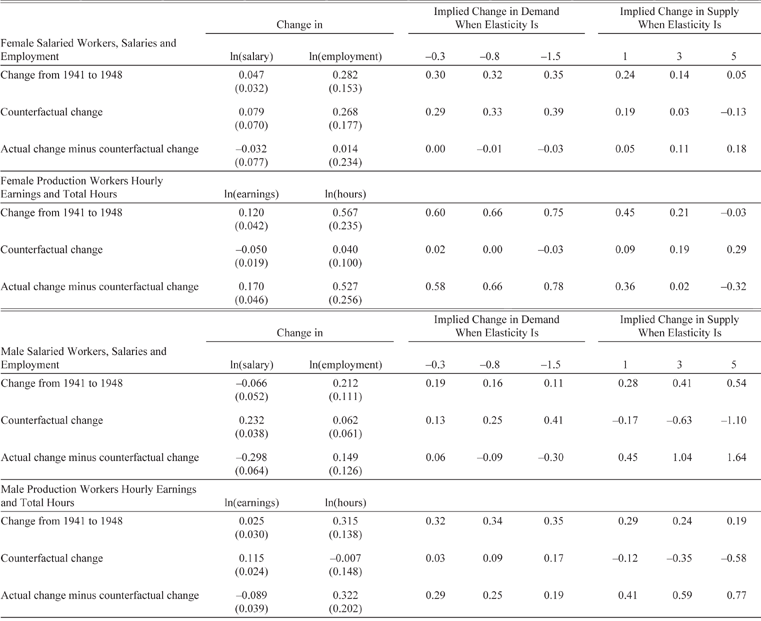
Changes in Residual Demand and Supply Between 1941 and 1948 After Controlling for Wages of Other Workers, Racial and Ethnic Mix, Value of Output Per Worker, Union Density, and Industry Mix with Comparisons to Counterfactual Estimates

Notes: Standard errors are in parentheses below the changes in ln(earnings), ln(salaries), ln(employment), and ln(hours). The changes and standard errors are based on the 1948 year fixed effect coefficients and standard errors from reduced-form panel regressions of each separately as a function of industry fixed effects and the factors listed in the title of the table from 1941 through 1948 in Online Appendix 6. The counterfactuals are based on the same types of regressions for the period 1923 through 1929, except that the coefficient and standard error for the 1929 coefficient is multiplied by 7/6 to allow the 1920s counterfactual six-year period to matchup with the seven-year period in the 1940s.
Source: See data section in the text.
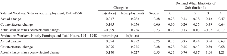
Changes in Relative Female/Male Residual Demand and Supply for Salaried and Wage Workers

Source: See data section in the text.
Even after controlling for the observable shift factors, there is a sizeable rise in the demand for female production workers that remains large after subtracting out the counterfactual. As with the raw information, the estimates of residual supply changes between 1941 and 1948 are somewhat uncertain and depend heavily on the supply elasticity chosen.
On the other hand, the pre- and post-war comparisons for female salaried workers are much smaller. The rise in residual demand between 1941 and 1948 of 0.32 in Table 5 is substantially smaller than the rise of 0.52 in Table 3. Meanwhile, the counterfactual change in demand was about the same at around 0.33 in both situations. As a result, the residual demand rose roughly the same amount between 1941 and 1948 as the counterfactual residual demand would have risen. Thus, there was virtually no change in the demand for female salaried workers relative to the 1920s counterfactual after controlling for the factors in the Xit vector and the industry fixed effects in equations (5a) and (5b).
In the residual counterfactual analysis of the demand for female workers relative to male workers in Table 6, a similar story arises. For salaried workers, the residual change in demand relative to the counterfactual is uncertain, ranging from a rise of 0.13 log points when the elasticity of substitution is 1 to −0.17 for an elasticity of substitution of 4. There is no doubt about the strong residual demand change for women relative to men in production, however. The rise in residual demand relative to the counterfactual ranges from 0.7 to 1.21 over the range from 1 to 4 in the substitution elasticity.
Why do we see the difference in the size of the shifts in residual demands for female production and salaried workers? Our sense is that females had long been performing office work for manufacturers in many industries while not being allowed on the production lines in those industries. Thus, they already had their foot in the door for many of the salaried jobs in ways that had not been available for female production workers.
How Much of the Rise in Earnings in the 1940s is Attributable to Individual Characteristics?
The analysis thus far has allowed us to control for several factors at the industry level that likely influenced the changes in demand in the 1940s. However, we have not directly controlled for changes in the averages of individual correlates that are common in earnings regressions, like education, age, marital status, and children. The use of the 1920s counterfactual provides one way to control for a number of these potential changes for the 1941 to 1950 period by subtracting the counterfactual growth rate in earnings and employment based on the rapid peace-time growth in the 1920s. Using estimates by Goldin and Katz (Reference Goldin and Katz2008, p. 21) for mean years of schooling of females by year of birth and the female age distributions in census years from Carter et al. (Reference Carter, Gartner and Haines2006, pp. 1–55), we estimate that mean years of schooling for females aged 15 to 65 rose by similar amounts between 1940 and 1950 (0.66 years) and between 1920 and 1930 (0.64 years). It therefore seems unlikely that changes in education among the female population was a major cause of the faster rise in demand for women workers in the 1940s than in the 1920s.
Even if the general rise of education was slower in the 1940s than in the 1920s, there is the possibility that the women who chose to work during WWII and afterward were older and more educated than women as a whole. This potential selection might also have led to higher earnings.Footnote 21 To explore the impact of schooling and other education characteristics further, we used the IPUMS census data for earnings from 1939 and 1949 for Pennsylvania to estimate regressions of ln(earnings) on individual characteristics (Ruggles et al. Reference Ruggles, Genadek and Goeken2015). We then performed Oaxaca decompositions to see how much of the change in average earnings for women in the 1940s was explained by changes in the mean individual characteristics and how much of the difference is left to be explained by other factors. The regression coefficients are qualitatively similar to other census earnings regressions in the literature and many of the coefficients for 1939 and 1949 are similar, even though 1939 was still a Depression year. They are reported along with the development of the Oaxaca decomposition in Online Appendix 3.
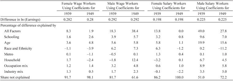
Only a small share of the rise in mean earnings for women between 1939 and 1949 can be explained by changes in the standard correlates in census earning regressions. Table 7 summarizes the shares of the differences in ln(earnings) explained by differences in the means of the correlates for all four groups of workers. The change in average schooling of female workers explains only 1.6 or 2.6 percent of the rise in earnings for wage workers and 0.8 or 3.2 percent for salaried workers. Differences in the average age explain a somewhat larger share than schooling at 3.6 or 4.8 for wage workers and 1.1 or 5.8 for salaried workers. Differences in average household characteristics like marital status and children present or ever born explain 1.7 or −2.4 percent for wage workers and −3.2 or 0.1 percent for salaried workers. After examining the impact of the changes in the means of all of the individual characteristics measures, the share of the rise in female earnings left to be explained by other factors is 98.1 or 91.7 percent for female wage workers and 100 or 86.2 percent for female salaried workers.
Difference in Mean LN (Real Earnings) Between 1939 and 1949 Explained by Differences in Means Using Ols Regression Coefficients From 1939 and 1949 for Female and Male Wage and Salary Workers

Notes and Sources: The Oaxaca decompositions are based on coefficients and means from regressions on Pennsylvania data from the IPUMS Census Samples for 1940 and 1950 (Ruggles et al. Reference Ruggles, Genadek and Goeken2015). The workers were between the ages of 10 and 65 and listed as “at work” in manufacturing industries working more than 35 hours per week in the census year and more than 40 weeks in the prior year with nominal incomes exceeding $350 in 1940 and $560 in 1950. Wage workers were operatives, craft workers, and laborers in the occupation listings and salaried workers were clerks, managers and professionals, and technical workers in the occupational listings. Annual earnings were used for salaried workers and hourly earnings for wage workers. The wages were adjusted to 1967 using the Consumer Price Index from U.S. Bureau of the Census (1975, series E-135). The percentage of the difference explained using the coefficient for 1939 for schooling was constructed by multiplying the schooling coefficient for 1939 by the difference in the mean schooling for the sample group between 1939 and 1949 and then dividing by the difference in ln (earnings) and multiplying by 100. The percentage explained by all factors is the sum of the percentages for the individual factors. The coefficients and means for each characteristic are reported in Appendix 4. The correlates in regression equations include years of schooling, age and age-squared, nonwhite, foreign born, native born with foreign parents, metro residence married spouse present, married spouse absent, divorced, widowed, children in home, children ever born, occupation categories, and industry categories.
When these unexplained percentages are multiplied by the residual changes in ln(earnings) from 1941 to 1948 in Table 5, the rise in the residual of ln(earnings) for female production workers after controlling for all factors on which we have information from Pennsylvania and the census is 0.097 or 0.104 log points. This residual change in earnings is 0.15 or 0.14 log points larger than the 1920s counterfactual change in residual earnings. When combined with the net effects for residual ln(employment), these changes are associated with large residual demand increases of 0.42 to 0.59 log points. When the same process is followed for female salaried workers, the residual change in ln(earnings) is 0.079 or 0.068 log points. Subtract the 1920s counterfactual and the relative rise in demand in the 1940s stays very close to zero. Given that the 1920s counterfactual has not been adjusted for individual characteristics in these calculations and that the rise in schooling was much larger in the 1920s, these new demand estimates are likely to be lower bound estimates of the shift in the 1940s relative to the 1920s.
Conclusions
During WWII, millions of women entered the labor force and worked in a wide range of jobs. We measure the extent to which the war experience altered the peacetime demand for women in industry. The results in Pennsylvania show that no matter how you measure the change in demand—the whole change, the change relative to a counterfactual, or actual and counterfactual changes for residual demand after controlling for a number of correlates—the war was associated with a substantial rise in the wartime demand and post-war demand for female production workers relative to the setting in 1941. The overall shift in demand, which is measured as the change in quantity demanded at a specific wage rate, boomed by more than 50 log points between 1941 and the war time peak in 1944. It then fell substantially after the war, but it still remained 16 to 23 log points higher than counterfactual trends from the 1920s.Footnote 22
After controlling for changes in the wages of other groups, shifts in labor demand based on product prices and general labor productivity, the ethnic mix, the industry mix, the occupation mix, education, age, and family structure, the residual component of demand for female production workers rose more than 42 log points more than the residual demand during the counterfactual period of the 1920s. Although there are many factors that could be included in the rise in residual demand during the 1940s, there are three likely candidates that we have not been able to measure. First, women gained extensive on-the-job training and experience in areas of manufacturing where they had not worked much before. Second, employers discovered that women were more productive on these jobs than they had previously thought. Third, employers likely found lower cost ways to adjust production to make better use of women’s adeptness in some areas and reduced the importance of strength (Pidgeon Reference Pidgeon1944, pp. 7–12). The U.S. Women’s Bureau performed a number of studies during the war years that documented how women were employed during the war in a variety of industries. A common statement was that employers, although initially skeptical, found that women had become highly effective employees.Footnote 23
The situation for female salaried workers was not as clear cut. Like the situation for female production workers, the demand and supply of female salaried workers boomed during the war, and both fell after the war. The longer-range impact of the war in peacetime is more uncertain. Comparisons of the raw numbers on salaries and employment to the counterfactual trend suggest that the demand and supply of labor in 1948 were about 12 to 20 log points higher than the predicted counterfactual. Such relative demand shifts occurred in all manufacturing sectors. After controlling for changes in a broad range of correlates, the residual component of demand for female salaried workers also rose substantially between 1941 and 1948–1950. However, the rise was about the same size as a counterfactual peacetime rise in residual demand during the 1920s. Thus, it seems likely that the war did not lead to a larger peacetime rise in the demand for female salaried workers in the way it did for female production workers. Even though the change in the level of demand for female salaried workers might not have been altered by the war, the demand for female salaried workers relative to male salaried workers rose substantially.
Our complex findings about the changes in demand associated with the war help explain why narrative histories came to conflicting conclusions about whether the war stimulated demand for female workers. The compilation of narratives shows that some women continued to work and some were let go, but the net effect on demand could not be determined without analyzing data on the number working and the wages paid. Further, the answer depends on whether the narrative focused on production line workers or salaried workers. Women had long been performing salaried work for manufacturers in many industries. Thus, they already had their foot in the door for many of the salaried jobs, and it is not surprising that the residual demand for their services rose little. In contrast, the war experience opened the door wide for women to work on production lines and contributed to a substantial rise in the demand for female production workers between 1941 and the late 1940s.