1. INTRODUCTION
This article deals with a real-world problem that might seem of recreational nature at first sight but that offers challenging questions of a general nature in a terminating two-person stochastic game. The problem concerns a real-world situation arising during a television game show. At the end of the show, the two remaining contestants have to play a two-person dice game. The contestants each sit behind a panel with a battery of buttons numbered 1,2,…, D (say, D = 10). In each stage of the game, all of the contestants must simultaneously press one of the buttons and the contestants cannot observe each other's decision. The number on the button pressed by the contestant is the number of dice that are thrown for the contestant. For each contestant, the score of the throw for that contestant is added to his/her total, provided that none of the dice in that throw showed the outcome 1; if the outcome is 1, no points are added to the current total of the candidate. The candidate who first reaches a total of G (say, G = 100) points is the winner. In the case that both candidates reach the goal of G points in the same move, the winner is the candidate who has the largest total. In the event of a tie, the winner is determined by a toss of a fair coin. At each stage of the game, both candidates have full information about his/her own current total and the current total of the opponent. The formulation of the game is such that it is zero-sum and stochastic. What does the optimal strategy look like? Do random actions appear? If so, when?
2. SOME PRELIMINARIES
Let us first look at the distribution of the number of points earned in a single throw with d dice. Define the random variable Yd as

Letting the random variable Xi denote the outcome shown by the ith dice, Yd equals X1 + ··· + Xd if none of X1,…, Xd equals 1, and Yd is 0 otherwise. The random variables X1,…, Xd are independent and identically distributed (i.i.d.). Moreover, given that Xi is not 1, the conditional distribution of Xi is the uniform distribution on the integers 2,3,…,6. This conditional distribution has expected value 4. The probability of not getting a 1 in a throw of d dice is

. Elementary calculations show that

The maximum of E(Yd) is easily found by looking at

The difference is positive for d < 5, is zero for d = 5, and is negative for d > 5. Hence, E(Yd) is maximized by taking d equal to 5 or 6. Heuristically, this result can also be obtained by marginal analysis. Given that you already have d dice in your hand, should you pick up another one? If one of the previous dice will give a 1, it is irrelevant what you do, so assume none of the other dice will give a 1. Then, on average, every one of them will contribute four points. So, in this situation with probability 1/6, you lose 4d points, and with probability 5/6, you win another four points. Thus, the expected gain is 20/6 − 4d/6 points, which becomes zero for d = 5.
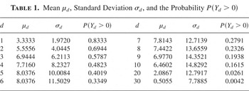
Table 1 gives the probability P(Yd > 0) together with the mean μd and standard deviation σd of the random variable Yd for various values of d.
Mean μd, Standard Deviation σd, and the Probability P(Yd > 0)

If you consider only the mean, the optimal number of dice is five or six for the situation of a single move. However, as the standard deviation shows, throwing with five or six dice is not the same. With six dice, the throw will be “riskier.” If you quickly need many points, then you have to take a risk so that throws with seven or more dice come into the picture.
Next, we discuss how to compute the probability distribution of Yd. For any d ≥ 1, let

Obviously,

and

with the convention r0(0) = 1 and ri(0) = 0 for i ≠ 0.
3. TWO ONE-PERSON GAMES
To get some insight, let us consider the following two one-person games. In the first one, we minimize the expected number of throws needed to reach G points. In the second one, we maximize the probability of reaching G in a given number of throws.
3.1. Expected Number of Throws
Define V(i) as the minimal expected number of additional throws when one still needs i additional points to reach the goal. Then, letting V(i) = 0 for i ≤ 0, we have the dynamic programming equation (cf. Derman [1])

or, equivalently,

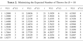
Table 2 gives the minimal expected number of throws and d*(i), the optimal number of dice to use in state i, where D = 10 is the maximum number of dice that can be thrown.
Minimizing the Expected Number of Throws for D = 10

As we see, the number of dice to use varies quite a lot. Even using seven dice is optimal in some states. Also note that in each of the states i = 1,…,28 in which the goal is to get at least i additional points, you use the number of dice that will hopefully give you i or more points, when there is no one among the outcome of the throw with those dice. In other words, in each state i with 1 ≤ i ≤ 28, you try to reach the goal in one “successful” throw. In each of the states i with 29 ≤ i ≤ 40, however, the optimal strategy is to reach the goal in two “successful” throws instead of one. Of course, if i gets large, you will only use throws with five or six dice, as these throws have the highest expected “value” (recall Table 1). As a result of this, we must also have limi→∞ V(i + 1) − V(i) = 1/8.0376, where 8.0376 is the expected number of points per throw with five or six dice.
3.2. Limited Number of Throws
Define p(l)(i) as the maximal probability of getting at least i additional points in at most L throws. Then, using standard dynamic programming, we have

where p(l)(i) = 1 for i ≤ 0 and p(0)(i) = 0 for i > 0.
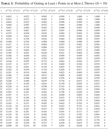
The results of a maximization with D = 10 are given in Table 3 for several values of the limit l on the number of allowed throws. In Table 3, d*(i,l) is the optimal number of dice to throw when you still need i points and you have l throws left. As we see, the number of dice to use is more regular (i.e., varies in a more monotonic way than in the case of minimizing the expected number of throws). You also see that starting at 40 with six throws left, you throw four dice. If the score turns out to be zero, you continue with five dice in the next throw. If then the score is 17 (so you have reached 23), you continue with four dice again, but if your score is 22 (so you are in 18), you continue with three dice, and so on.
Probability of Getting at Least i Points in at Most L Throws (D = 10)

It can be noted from Table 3 that for fixed values of i the maximal probability p(l)(i) as function of l has an S-shaped form; that is, for each i, there is an l(i) such that p(l)(i) is convex for l < l(i) and concave for l > l(i). Computations of p(l)(i) for larger values of i and l affirmed this behavior. It is our conjecture that, indeed, p(l)(i) is always S-shaped.
To the contrary, the behavior of p(l)(i) for fixed l as a function of i is quite irregular. We have also found that the somewhat surprising result that for l equal to 5 or 6, the value of d*(i,l) is not monotone. For l = 5, it first increases to 10 (the maximal number of dice) for i = 79,…,89, then decreases to 9 for i = 90, 91, then to 8 for i = 92, 93, 94, after which it again increases via 9 to 10. For l = 6, it increases to 8 for i = 74,…,82, then decreases to 7 for i = 83,…,91, after which it again increases via 8 and 9 to 10.
4. THE TWO-PERSON STOCHASTIC GAME
The rules of the game state that in each throw, simultaneously the two players have to decide on the number of dice to use, without seeing what the opponent is doing but knowing and using the scores so far. So, after a number of throws, player 1 still needs a points and player 2 needs b points. Thus, the state space is two dimensional. If now player 1 decides to use k dice and player 2 uses l, then the state changes from (a,b) to (a − i, b − j) with probability qi(k)qj(l).
The game is a stochastic terminating zero-sum game. If we assume that the number of dice to be used in each throw is limited by some number, D say (D = 10 in the television game show), then the game can be solved recursively by dynamic programming.
The value of the game is equal to the probability that player 1 wins minus the probability that player 2 wins, given that both players play optimally. Define

We want to determine V(a,b) for both a and b positive (and less than or equal to G) and the optimal, possibly randomized, actions that guarantee this value.
4.1. Randomized Actions
The first question might be: Do the players have to randomize the number of dice to use in a throw? Some insight is already gained by just looking at the game starting in (1,1). Knowing that the value of this symmetric state has to be zero, we can check whether there is a “deterministic move” (i.e., using a fixed number of dice) that guarantees the value zero. If there would be an optimal deterministic throw, then we should have for some d ≤ D and for all l,

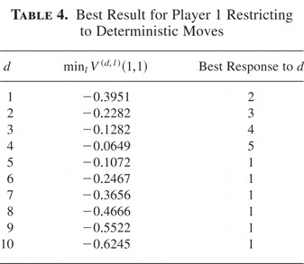
Computing minl V(d,l) (1,1) for all d leads to the results in Table 4.
Best Result for Player 1 Restricting to Deterministic Moves

So, there is no optimal number of dice. The best number is four, but even then, the best you can get is −0.0649. If your opponent knows the number of dice you use, it is optimal for him to use one die more, unless you use five or more dice; then his optimal choice is one die. Thus, randomization is necessary.
4.2. The Optimality Equation
The two-person zero-sum stochastic game is in fact a terminating, even contracting game. In each move (throw of the two players), the state of the game gets closer to the payoff zone: the set of states (a,b) with min{a,b} ≤ 0 (define the distance from (a,b) to the payoff zone as a + b if both a and b are positive; then with a probability of at least 1 − (q0(D))2, the distance decreases by at least 2).
The value of the game and the optimal moves of the two players can be computed by repeatedly solving the appropriate matrix games. Let x = (x1,x2,…, xD) be a randomized move for player 1; that is, player 1 throws d dice with probability xd, where [sum ]d xd = 1. The first approach to think of is to recursively compute V(a,b) via a sequence of LP-problems, starting in (a,b) = (1,1) and working backward, step by step, until (a,b) = (G,G). This requires solving the optimization problem:

where, for i + j > 0, the values V(a − i, b − j) have been computed earlier and, hence, are known. (V is unrestricted in sign.) However, this optimization problem is not exactly an LP-problem because of the nonlinear term [sum ]d xd q0(d)q0(l)V.
To make an LP-approach possible, we proceed as follows. Define V(n)(a,b) as the value of the game if it is played at most n times with a terminal reward 0, if after n steps the game has not yet reached the payoff zone. Thus, V(0)(a,b) := 0 if a > 0 and b > 0. Also, define

with the convention that, for n ≥ 0 and a ≤ 0 or b ≤ 0, V(n)(a,b) = V(a,b) with V(a,b) as defined in (1). Then, in iteration n for state (a,b), the value of the game and an optimal move for player 1 can be obtained from the following LP-problem for a matrix game (cf. Maitra and Sudderth [2]):

The optimal value V satisfies V = V(n)(a,b) and the optimal x(n)(a,b) represents an optimal move for player 1 in state (a,b) in iteration n. V(n)(a,x,b,l) converges exponentially fast to the value of the game, and x(n) is nearly optimal for n sufficiently large. Similarly, we can compute a (nearly) optimal strategy for player 2. Of course, for symmetry reasons, the optimal move for player 2 in (a,b) is the same as the optimal move for player 1 in (b,a).
Remark. In order to profit from the contracting properties of the dynamic programming scheme for Vn, one could introduce a so-called weighted supremum norm μ. Defining μ(a,b) = αa+b for some α > 1, the model will be contracting with respect to the μ-norm and nearly optimal strategies and upper and lower bounds can be computed from the difference between V(n+1) and V(n) (cf. van der Wal and Wessels [3]).
4.3. Numerical Results
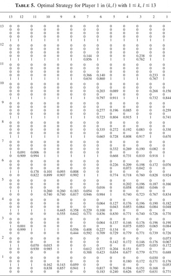
In Table 5 we present some results for the optimal strategy for the case that the maximum number of dice that can be thrown is D = 5. Table 5 should be read as follows. If, for instance, player 1 still needs one point and player 2 needs three points, then player 1 will use two, four, or five dice with probabilities 0.172, 0.151, and 0.677, respectively.
Optimal Strategy for Player 1 in (k,l) with 1 ≤ k, l ≤ 13

Our numerical results indicate that the optimal strategy has certain monotonicity properties. It would be nice to have a theoretical proof for the monotonicity properties. Also, it appears from the calculations in Table 5 that for states above 13, the players use nonrandomized decisions only. Again, this is a kind of turnpike result one would expect, but it would be nice if it could be proved theoretically. What we also see from Table 5 is the following. For instance, in state (5,13), player 1 will use four dice and player 2 will use five dice. So both players use more dice than needed to reach the payoff zone in order to beat the other player in case neither one of them throws a 1.
5. VARIANTS
There are various possible modifications of this game:
- Player 2 uses the optimal strategy with respect to one of the one-person games discussed earlier. What is the optimal response for player 1 and how does this increase “his value”? This “game” can still be solved by ordinary dynamic programming.
- Suppose that the players alternatingly throw a number of dice, where at the beginning of the show, a coin is flipped to decide which player starts. Again, a simple dynamic programming algorithm suffices to obtain the optimal strategy.
- Suppose that a player gets not only a score of zero but also loses all (or some of) the points collected so far if there is an outcome 1 in the throw of his dice.
- Suppose the players know the outcomes of their own throws, but do not know what the other player has been doing at all. This is a game with imperfect information. Is it possible to determine an optimal strategy?
- Suppose that, in addition to the previous situation, you also know how many dice your opponent has used. This, too, is a game with imperfect information.