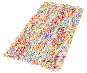


1 Introduction
The dynamics of wall shear stress,  $\unicode[STIX]{x1D70F}_{w}$, over smooth and rough walls is of central importance in the determination and understanding of drag and has been the focus of experimental and numerical studies over many decades. The skin-friction drag, or the mean wall shear stress,
 $\bar{\unicode[STIX]{x1D70F}}_{w}$, in smooth-wall turbulence has received significant attention and its dependence on Reynolds number (
 $Re$) has been extensively investigated and well documented (Schlichting (Reference Schlichting1968), Dean (Reference Dean1978), Colella & Keith (Reference Colella and Keith2003), Wu & Moin (Reference Wu and Moin2009), Schlatter & Örlü (Reference Schlatter and Örlü2010), Hwang (Reference Hwang2013), amongst others).
However, surface roughness greatly increases the complexity of the near-wall turbulence generation mechanism. Since the pioneer experiments by Nikuradse (Reference Nikuradse1933) in turbulent pipe flows with sand-grain roughness, the effects of surface roughness on wall turbulence have been investigated over the past few decades for a wide variety of two-dimensional (2-D) (Krogstad & Antonia Reference Krogstad and Antonia1999; Leonardi et al. Reference Leonardi, Orlandi, Smalley, Djenidi and Antonia2003; Ashrafian, Andersson & Manhart Reference Ashrafian, Andersson and Manhart2004; Ikeda & Durbin Reference Ikeda and Durbin2007; Lee & Sung Reference Lee and Sung2007; Burattini, Leonardi & Orlandi Reference Burattini, Leonardi and Orlandi2008) and three-dimensional (3-D) roughness topographies (Cheng & Castro Reference Cheng and Castro2002; Flack, Schultz & Shapiro Reference Flack, Schultz and Shapiro2005; Coceal et al. Reference Coceal, Dobre, Thomas and Belcher2007; Leonardi & Castro Reference Leonardi and Castro2010; Yuan & Piomelli Reference Yuan and Piomelli2014), and even more realistic irregular roughness (Wu & Christensen Reference Wu and Christensen2007, Reference Wu and Christensen2010; Busse, Lutzner & Sandham Reference Busse, Lutzner and Sandham2015). It is well established that the presence of roughness elements enhances drag at the wall (except for flow-aligned riblets, which reduce the drag (Choi, Moin & Kim (Reference Choi, Moin and Kim1993), Orlandi, Leonardi & Antonia (Reference Orlandi, Leonardi and Antonia2006), for example)), as discussed comprehensively in the recent review by Jiménez (Reference Jiménez2004).
The increased drag due to roughness leads to a downward shift of the mean streamwise velocity profile in the logarithmic region compared to smooth-wall flow and this downward shift is well known as the roughness function  $\unicode[STIX]{x0394}U^{+}$ (the superscript ‘+’ denotes normalization in wall units). Detailed surveys of the relationship between the roughness function and the roughness height
 $k^{+}$ for various surface geometries (Raupach, Antonia & Rajagopalan Reference Raupach, Antonia and Rajagopalan1991) showed that flow remains hydraulically smooth (i.e.
 $\unicode[STIX]{x0394}U^{+}=0$) for small
 $k^{+}$, where viscous dissipation is sufficient to negate any perturbations induced by surface roughness, but, for large
 $k^{+}$,
 $\unicode[STIX]{x0394}U^{+}$ reaches an asymptote region where the flow is termed fully rough and the skin friction becomes independent of
 $Re$. This transition to fully rough conditions is predominantly due to the growing dominance of form-drag contributions to the overall drag over viscous-drag contributions with increasing
 $k^{+}$. At intermediate heights, the flow is termed transitionally rough whereby both form- and viscous-drag contributions are significant and strongly coupled in the roughness sublayer. The equivalent sand-grain roughness height
 $k_{s}^{+}$ (the roughness height that produces the same roughness function as that of sand grains of size
 $k_{s}$), which serves merely as an a posteriori measure of the roughness effect in most engineering applications, is shown to collapse
 $\unicode[STIX]{x0394}U^{+}$ onto the same asymptote line in the fully rough regime but is unable to collapse surfaces that are transitional rough (Jiménez Reference Jiménez2004; Flack & Schultz Reference Flack and Schultz2010). The transition from hydraulically smooth to fully rough conditions with increasing
 $k_{s}^{+}$ is dependent on the details of the roughness topography beyond simply its characteristic height, and it is still not well understood.
It is evident, however, that the characteristic roughness height alone is not sufficient to fully characterize the overall drag induced by a roughness topography. For example, the element packing density was considered by Leonardi et al. (Reference Leonardi, Orlandi, Smalley, Djenidi and Antonia2003) and Djenidi et al. (Reference Djenidi, Antonia, Amielh and Anselmet2008) for 2-D arrays of transverse square bars and they agreed that the largest drag is produced for streamwise bar separation  $\unicode[STIX]{x1D706}/k=8$. In addition, Leonardi & Castro (Reference Leonardi and Castro2010) investigated 3-D arrays of staggered cubes and reported that the peak drag occurs at a plan surface coverage of 15 %. Depending on the details of roughness geometry, a surface topography is commonly called a ‘k-type’ roughness when the elements are sparsely spaced and the behaviour of
 $\unicode[STIX]{x0394}U^{+}$ depends on
 $k^{+}$. This is in contrast to the ‘d-type’ roughness, first classified by Perry, Schofield & Joubert (Reference Perry, Schofield and Joubert1969), in which surfaces are characterized by narrowly spaced or densely packed roughness elements and
 $\unicode[STIX]{x0394}U^{+}$ is instead dependent upon the outer length scale of the flow (boundary layer thickness, channel half-height or pipe diameter). Other geometrical parameters, such as the effective slope, skewness and kurtosis, etc., can also influence the behaviours of drag (Flack & Schultz Reference Flack and Schultz2010), and it clearly requires more scrutiny to correlate the physical attributes of a roughness topography to the drag.
While much effort is devoted to the mean wall shear stress in smooth- and rough-wall-bounded turbulent flows, less is known about the fluctuations in the wall shear stress. Higher-order statistics of  $\unicode[STIX]{x1D70F}_{w}$, such as its root-mean-square (r.m.s.) value, skewness, etc., become relevant in multiscale modelling of turbulent flows, particularly in large-eddy simulation (LES), where
 $\bar{\unicode[STIX]{x1D70F}}_{w}$ does not embody sufficient statistical information about the nature of the drag variations. This issue is exacerbated when dealing with rough walls, where drag embodies a complex interplay between viscous and pressure effects depending upon the characteristics of the roughness and the
 $Re$ of the flow.
Early smooth-wall experiments reported that the wall shear stress r.m.s. in wall units scatters around a classical value of 0.4, but shows contradictory trends with increasing  $Re$, primarily because of insufficient spatial resolution and frequency response of measurement instruments at high
 $Re$ (Alfredsson et al. Reference Alfredsson, Johansson, Haritonidis and Eckelmann1988; Österlund Reference Österlund1999; Colella & Keith Reference Colella and Keith2003). Direct numerical simulation (DNS) of smooth-wall-bounded turbulent flows, although limited to low to moderate
 $Re$, have improved our understanding in this regard. Örlü & Schlatter (Reference Örlü and Schlatter2011) compiled data from numerical and experimental studies of wall shear stress r.m.s. and showed a consistent increasing trend with
 $Re$. This enhanced wall shear stress r.m.s. is linked to the large-scale motions (LSMs) and very-large-scale motions (VLSMs) residing in the outer region of high-
 $Re$ flows (Hutchins et al. Reference Hutchins, Monty, Ganapathisubramani, Ng and Marusic2011; Örlü & Schlatter Reference Örlü and Schlatter2011). These large-scale structures, which have been identified in all types of turbulent flows (Kim & Adrian (Reference Kim and Adrian1999), Christensen & Adrian (Reference Christensen and Adrian2001), del Álamo & Jiménez (Reference del Álamo and Jiménez2003), Tomkins & Adrian (Reference Tomkins and Adrian2003), Hutchins & Marusic (Reference Hutchins and Marusic2007a), Monty et al. (Reference Monty, Stewart, Williams and Chong2007), Mejia-Alvarez, Wu & Christensen (Reference Mejia-Alvarez, Wu and Christensen2014), Barros & Christensen (Reference Barros and Christensen2019), amongst others) are strongly dependent on
 $Re$, with their energy content and influence increasing as
 $Re$ increases (Kim & Adrian Reference Kim and Adrian1999; Guala, Hommema & Adrian Reference Guala, Hommema and Adrian2006; Balakumar & Adrian Reference Balakumar and Adrian2007; Hutchins & Marusic Reference Hutchins and Marusic2007a,Reference Hutchins and Marusicb).
The influence, or ‘footprint’, of outer-layer, large-scale events can penetrate deep into the near-wall region, identified in the 2-D pre-multiplied spectra of the wall shear stress as a low-wavenumber superposition effect that increases with increasing  $Re$ (Örlü & Schlatter Reference Örlü and Schlatter2011). This behaviour is in agreement with the attached-eddy hypothesis (Townsend Reference Townsend1976). Particle image velocimetry and hot-wire measurements in turbulent boundary layers (TBLs) have shown that packets of self-similar hairpin vortices grow in wall-bounded flows with length scales proportional to the distance from the wall and are organized coherently into large-scale structures (Kim & Adrian Reference Kim and Adrian1999; Adrian, Meinhart & Tomkins Reference Adrian, Meinhart and Tomkins2000; Christensen & Adrian Reference Christensen and Adrian2001), which appear as meandering elongated streamwise low- and high-momentum regions (LMRs and HMRs) near the wall, leading to large-scale variations in the wall shear stress (Abe, Kawamura & Choi Reference Abe, Kawamura and Choi2004; Hutchins & Marusic Reference Hutchins and Marusic2007a; Hutchins et al. Reference Hutchins, Monty, Ganapathisubramani, Ng and Marusic2011). Recent experiments in high-
 $Re$ TBLs have also revealed that the near-wall, small-scale turbulence is amplitude-modulated by LSMs that reside in the outer layer through a nonlinear process, the intensity of which increases with
 $Re$ (Hutchins & Marusic Reference Hutchins and Marusic2007b; Mathis, Hutchins & Marusic Reference Mathis, Hutchins and Marusic2009). Coupling the effects of superposition and modulation of the LSMs on the near-wall small scales, Mathis, Hutchins & Marusic (Reference Mathis, Hutchins and Marusic2011) proposed an empirical model that was able to reproduce the near-wall streamwise velocity statistics given only information of the LSMs in the log region, producing excellent prediction of statistics in comparison with the original data over a wide range of
 $Re$. While the predictive model was first developed for streamwise velocity fluctuations, Mathis et al. (Reference Mathis, Marusic, Chernyshenko and Hutchins2013) extended this framework to predict fluctuating wall shear stress assuming that the inner–outer interaction is quasi-steady such that the near-wall turbulence is affected by the slowly varying large-scale structures in the outer region. The predicted fluctuation magnitude of the wall shear stress showed good agreement with the
 $Re$ trends reported by Schlatter & Örlü (Reference Schlatter and Örlü2010), an encouraging result for advancing the near-wall modelling of turbulent flows.
Outer-layer similarity between smooth- and rough-wall turbulence has been previously documented for a variety of roughness topographies (Krogstad & Antonia (Reference Krogstad and Antonia1999), Flack et al. (Reference Flack, Schultz and Shapiro2005), Wu & Christensen (Reference Wu and Christensen2007), Volino, Schultz & Flack (Reference Volino, Schultz and Flack2007, Reference Volino, Schultz and Flack2011), Leonardi & Castro (Reference Leonardi and Castro2010), Chung, Monty & Ooi (Reference Chung, Monty and Ooi2014) amongst others), provided that  $Re$ is sufficiently high and the scale separation between the characteristic roughness scale and the outer scale of the flow (boundary layer thickness, for example) is large, in accordance with Townsend’s wall similarity hypothesis (Townsend Reference Townsend1976). In this regard, roughness effects are mainly confined to the inner layer, whereas no substantial variations are observed in the outer flow. This similarity has been observed in a variety of single-point statistics, including the mean streamwise velocity and various components of Reynolds stresses. The structural attributes of the outer layer also appear similar between the smooth and rough walls (Wu & Christensen Reference Wu and Christensen2010; Mejia-Alvarez et al. Reference Mejia-Alvarez, Wu and Christensen2014; Barros & Christensen Reference Barros and Christensen2019). Two-point spatial correlations of velocity fluctuations showed similar streamwise and spanwise extents of the large-scale structures outside the roughness sublayer, although a weak shortening of the streamwise length was observed close to the roughness in comparison with smooth-wall flow (Krogstad & Antonia Reference Krogstad and Antonia1994; Volino et al. Reference Volino, Schultz and Flack2007; Wu & Christensen Reference Wu and Christensen2010; Volino et al. Reference Volino, Schultz and Flack2011). Coceal et al. (Reference Coceal, Dobre, Thomas and Belcher2007) performed DNS of turbulent flow over cubical roughness and also reported longer streamwise length of the LMRs over the smooth wall compared to the rough wall, with the effect being largest near the roughness and diminishing away from the wall. Thus, wall similarity observed in the outer region plays a crucial role in practical engineering problems involving modelling of rough-wall flows. In LES of rough-wall flow, it is explicitly required to specify the roughness function in order to derive the velocity scaling and mean wall shear stress, both of which are necessary to set the boundary conditions for the outer region to be resolved. There is currently no first-principles strategy to determine the roughness function based solely on the statistics of the outer flow and the surface topography; empiricism is currently required. Furthermore, more advanced turbulence modelling may also benefit from incorporating the aforementioned inner–outer interactions between large-scale and small-scale motions, accounting for the response of wall shear stress to increasing
 $Re$.
This study is a continuation of our recent DNS study of turbulent channel flow over hemispherical roughness (Wu, Christensen & Pantano Reference Wu, Christensen and Pantano2019), which focused on modelling inner–outer flow interactions by leveraging the framework of amplitude modulation (AM). In the present study, wall shear stress is extracted from the DNS and the near-wall flow structures are investigated using flow visualizations with the aid of spherical harmonics to demonstrate the dominant flow features and associated physical interpretations for various roughness packing densities. In addition, we extend the wall shear stress model pioneered by Mathis et al. (Reference Mathis, Marusic, Chernyshenko and Hutchins2013) to rough-wall flows with the intent of modelling the characteristics of the universal wall shear stress in terms of the conditionally spatially averaged statistics of the mean and fluctuations. The behaviours of wall shear stress statistics to different averaging extents are also investigated to assist wall modelling in the context of LES.
2 Simulation description
Recently, Wu et al. (Reference Wu, Christensen and Pantano2019) performed DNS of turbulent channel flow over rough walls, where both walls were roughened by a mat of hexagonally packed hemispheres. The roughness height,  $k$, is given by the radius of the hemisphere and
 $d$ is the spacing between two hemispheres from centre to centre. The computational domain was constructed using body-fitted spectral elements where regions surrounding the roughness elements employed denser elements to ensure sufficient resolution within the roughness sublayer.
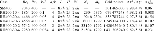
Parameters of the simulations. The roughness height  $k$ is the radius of the hemispheres;
 $d$ is the distance between hemispheres measured from centre to centre;
 $h$ is the half-channel height. The bulk Reynolds number is
 $Re_{b}=U_{b}h/\unicode[STIX]{x1D708}$; the friction Reynolds number is
 $Re_{\unicode[STIX]{x1D70F}}=u_{\unicode[STIX]{x1D70F}}h/\unicode[STIX]{x1D708}$; the roughness-height Reynolds numbers are kept the same at
 $k^{+}=u_{\unicode[STIX]{x1D70F}}k/\unicode[STIX]{x1D708}=20$ for all rough-wall cases. The total number of hemispheres is
 $N_{h}$ and
 $M_{h}$ is the number of grid points per roughness element on the hemisphere. Finally,
 $\unicode[STIX]{x0394}y_{min}^{+}$ is computed at the apex of the hemisphere.

Table 1 summarizes the details of the computation parameters used in all simulations. The dimensions of the domain for all cases were  $L=8\unicode[STIX]{x03C0}h$,
 $H=2h$ and
 $W=2\unicode[STIX]{x03C0}h$ in the streamwise (
 $x$), wall-normal (
 $y$) and spanwise (
 $z$) directions, respectively, where
 $h$ is the half-channel height. The boundary conditions were no-slip on both walls and periodic in the streamwise and spanwise directions.
Simulations were performed at  $Re_{\unicode[STIX]{x1D70F}}=u_{\unicode[STIX]{x1D70F}}h/\unicode[STIX]{x1D708}=200$,
 $400$ and
 $600$, where
 $u_{\unicode[STIX]{x1D70F}}$ is the friction velocity defined by
 $u_{\unicode[STIX]{x1D70F}}=\sqrt{\bar{\unicode[STIX]{x1D70F}}_{w}/\unicode[STIX]{x1D70C}}$. The mean wall shear stress,
 $\bar{\unicode[STIX]{x1D70F}}_{w}$, was calculated as the total drag per unit flat surface area of the wall. Note that using a body-fitted mesh allowed accurate calculation of the pressure and viscous forces, projected along the flow direction, over the wall. Three rough-wall simulations were performed at a friction Reynolds number
 $Re_{\unicode[STIX]{x1D70F}}=400$, yielding an inner-scaled roughness height
 $k^{+}=20$, while the pitch-to-height ratio between roughness elements was varied in the range
 $d/k=2$ to 4. Two more simulations were performed at
 $Re_{\unicode[STIX]{x1D70F}}=200$ and
 $600$ to investigate the Reynolds number trends while maintaining
 $k^{+}=20$ and
 $d/k=4$. Based on the equivalent sand-grain roughness height
 $5<k_{s}^{+}<70$ for all cases, the rough surfaces studied herein are still in the transitional rough regime. Additionally, a smooth-wall channel flow DNS was performed at
 $Re_{\unicode[STIX]{x1D70F}}=400$ for comparison purposes. Throughout the paper, the smooth- and rough-wall simulations are denoted by SM and RH, respectively. All data presented herein were obtained from these simulations. Further details about the computational mesh and numerical method as well as the criteria for statistical convergence of the flow can be found in Wu et al. (Reference Wu, Christensen and Pantano2019).
3 Wall shear stress analysis
Near-wall turbulence in smooth-wall flows at low and moderate  $Re$ is well known to be governed by a nonlinear self-sustaining process (Jiménez & Moin Reference Jiménez and Moin1991; Hamilton, Kim & Waleffe Reference Hamilton, Kim and Waleffe1995), associated with streamwise-elongated low-speed streaks (Kline et al. Reference Kline, Reynolds, Schraub and Runstadler1967) and shorter quasi-streamwise vortices (Kim, Moin & Moser Reference Kim, Moin and Moser1987; Jeong et al. Reference Jeong, Hussain, Schoppa and Kim1997). Collective evidence has revealed that these quasi-streamwise vortices are the legs of the self-similar hairpin vortices that populate the logarithmic layer and above, with length scales proportional to the distance from the wall (Adrian et al. Reference Adrian, Meinhart and Tomkins2000; Tomkins & Adrian Reference Tomkins and Adrian2003; Adrian Reference Adrian2007). Originating at the wall, a hierarchy of hairpin vortices grows into coherent streamwise-aligned packets inclined towards the downstream direction and extend to the centre of the flow, responsible for the intense ejections of low-momentum fluid away from the wall (Zhou et al. Reference Zhou, Adrian, Balachandar and Kendall1999; Christensen & Adrian Reference Christensen and Adrian2001). With the presence of roughness at the wall, the inner layer (driven by viscous effects) is effectively replaced by the roughness sublayer (Raupach et al. Reference Raupach, Antonia and Rajagopalan1991), where the mechanism of turbulence generation and sustainment depends on the characteristics of the roughness and
 $Re$. Previous studies have shown that the streamwise-elongated LMRs bordered by the hairpin packets are also present in wall-bounded flows over rough surfaces (Volino et al. Reference Volino, Schultz and Flack2007; Wu & Christensen Reference Wu and Christensen2010; Mejia-Alvarez et al. Reference Mejia-Alvarez, Wu and Christensen2014). Here, we will discuss the structures that are observed for the hemispherical roughness studied as well as the statistics of the wall shear stress.
3.1 Turbulent structures within the roughness sublayer
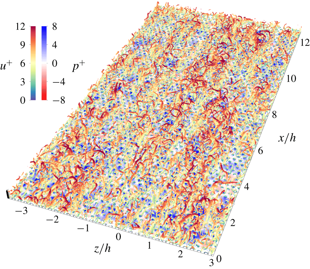
Flow visualization of vortical structures within the roughness sublayer,  $0<y^{+}<100$, for RH400-20-4 using isosurfaces of
 $\unicode[STIX]{x1D706}_{2}^{+}=-0.005$, coloured by the streamwise velocity
 $u^{+}$. The instantaneous pressure
 $p^{+}$ is also shown in the background.

Figure 1 presents a flow visualization of vortical structures within the roughness sublayer,  $0<y^{+}<100$, for RH400-20-4. These structures are identified using the
 $\unicode[STIX]{x1D706}_{2}$-criterion developed by Jeong & Hussain (Reference Jeong and Hussain1995) and are shown as isosurfaces of
 $\unicode[STIX]{x1D706}_{2}^{+}=\unicode[STIX]{x1D708}^{2}\unicode[STIX]{x1D706}_{2}/u_{\unicode[STIX]{x1D70F}}^{4}=-0.005$, coloured by the inner-scaled streamwise velocity
 $u^{+}$. In principle, there is no ambiguity in how to select the values to render the isosurfaces, as the criterion
 $\unicode[STIX]{x1D706}_{2}^{+}<0$ is scale-invariant (Tufo et al. Reference Tufo, Fischer, Papka and Blom1999). In practice, a slightly negative value of
 $\unicode[STIX]{x1D706}_{2}^{+}$ is selected for the isosurface to avoid noisy regions where the velocity is close to zero. Also shown in the background is the instantaneous pressure
 $p^{+}$ with a different colour scheme. Similar to smooth-wall flows, the near-wall region of this rough-wall flow is populated by trains of hairpin-like vortices that appear to be one-sided ‘cane-like’ or two-sided asymmetric ‘omega-like’ vortices, consistent with the observations reported by Tomkins & Adrian (Reference Tomkins and Adrian2003) and Coceal et al. (Reference Coceal, Dobre, Thomas and Belcher2007). The clusters of hairpin vortices are not randomly distributed near the wall but instead are organized coherently into packets that extend multiple outer length scales
 $h$ downstream, with a spanwise width of approximately
 $(1{-}1.5)h$. It is also worth noting that the spatial organization of the hairpin packets is highly correlated with the streamwise-elongated regions of high and low pressure (also coincident with regions of large vertical velocity gradient across the boundary layer). This spanwise-alternating pattern of high- and low-pressure patches is clearly reminiscent of the spanwise-alternating HMRs and LMRs found previously in both smooth- and rough-wall flows, representing the large-scale signature from outer-layer events (Ganapathisubramani, Longmire & Marusic (Reference Ganapathisubramani, Longmire and Marusic2003), Tomkins & Adrian (Reference Tomkins and Adrian2003), Ganapathisubramani et al. (Reference Ganapathisubramani, Hutchins, Hambleton, Longmire and Marusic2005), Volino et al. (Reference Volino, Schultz and Flack2007), Wu & Christensen (Reference Wu and Christensen2010), Mejia-Alvarez et al. (Reference Mejia-Alvarez, Wu and Christensen2014) among others).
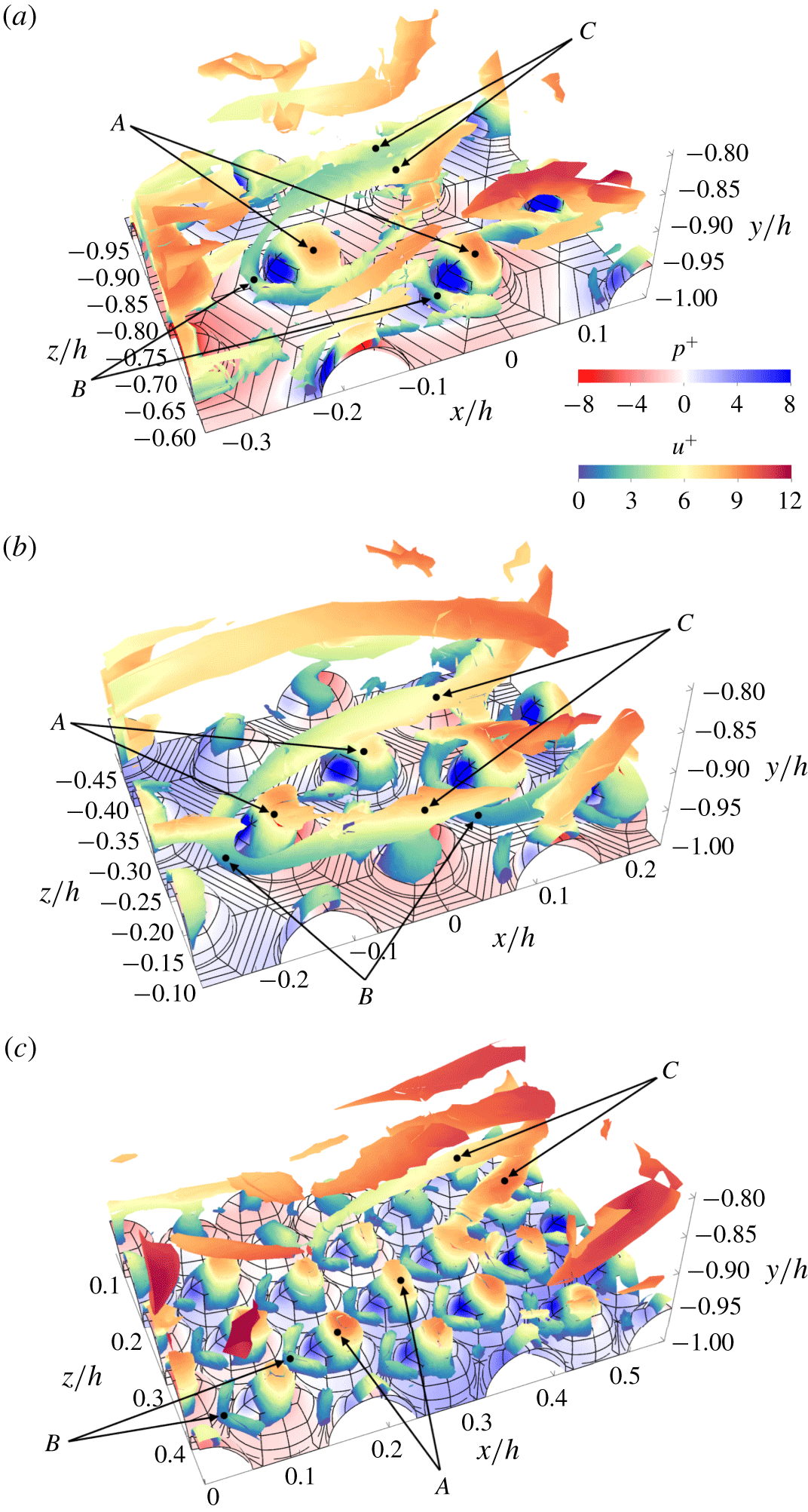
Vortical structures in the vicinity of hemispherical roughness for all roughness topographies at  $Re_{\unicode[STIX]{x1D70F}}=400$, identified by the isosurfaces of
 $\unicode[STIX]{x1D706}_{2}^{+}=-0.005$ and coloured by the streamwise velocity
 $u^{+}$. Instantaneous pressure
 $p^{+}$ is also shown in the background superimposed on the roughness geometry. Typical surface vortical structures, ‘horseshoe’ vortices and trailing vorticity loops are marked by the letters A, B and C, respectively.

Figure 2(a) illustrates the vortical structures spatially coincident with the individual hemispheres for RH400-20-4, identified using the  $\unicode[STIX]{x1D706}_{2}$-criterion. In addition to the hairpin vortex packets observed within and outside the roughness sublayer, a prevailing surface vortical structure (marked A) is identified in the vicinity of hemispheres, which spawns immediately upstream of each hemisphere and covers the hemisphere’s frontal surface. Previous experimental studies in TBLs with a single large hemispherical dome mounted on the wall (Taniguchi et al. Reference Taniguchi, Sakamoto, Kiya and Arie1982; Savory & Toy Reference Savory and Toy1986a,Reference Savory and Toyb) suggest that this vortical structure is induced by the generation of surface vorticity between the frontal stagnation and flow separation points, due to the surface pressure gradient. Unlike the self-similar hairpin vortices whose length scales are linearly proportional to distance from the wall, the induced frontal vortices are likely to scale with the height of the roughness elements. Similarly, the vortical structures in the roughness sublayer of RH400-20-3 and RH400-20-2 are shown in figure 2(b) and 2(c), respectively. It is found that this structural development is strongly affected by roughness element spacing. As the distance between elements decreases, the vertical velocity gradient across the roughness sublayer decreases as flow is lifted upwards by the roughness. Consequently, the stagnation point upstream of each hemisphere climbs uphill, resulting in a reduced pressure gradient induced by the roughness elements. Since the concentration of vorticity lines is controlled by the pressure gradient, it is seen that the surface area of the hemisphere covered by the vortical structures dwindles from almost the entire frontal surface for RH400-20-4 to only the tip of each hemisphere for RH400-20-2.
Furthermore, there is an additional type of vortical structure developed upstream of each hemisphere but less frequently seen compared to the prevailing surface vortical structures. When the roughness elements are far apart as shown in figure 2(a), the oncoming boundary layer vorticity lines accumulate below the frontal stagnation point and curl around each roughness element, forming a so-called ‘horseshoe’ vortex (marked B), or alternatively termed the ‘standing’ vortex by Acarlar & Smith (Reference Acarlar and Smith1987). These horseshoe vortices have also been investigated previously for isolated hemispheres immersed in a TBL (Taniguchi et al. Reference Taniguchi, Sakamoto, Kiya and Arie1982; Savory & Toy Reference Savory and Toy1986a; Suzuki et al. Reference Suzuki, Kiya, Sampo and Naka1987), which share similar aerodynamic characteristics with most commonly studied 3-D roughness shapes, e.g. cubes, cones, pyramids, etc. (Castro & Robins Reference Castro and Robins1977; Ballio, Bettoni & Franzetti Reference Ballio, Bettoni and Franzetti1998; Martinuzzi & AbuOmar Reference Martinuzzi and Abuomar2003; Martinuzzi, AbuOmar & Savory Reference Martinuzzi, Abuomar and Savory2007). The vorticity lines in the wake of hemispheres appear to curl around each other and form long trailing vorticity loops (marked C) downstream, consistent with the observations by Savory & Toy (Reference Savory and Toy1986a). While the trailing vorticity loops are clearly attached to the wall when only one large roughness element is considered, the hexagonal packing of hemispheres studied herein distorts the trailing vorticity loops, redirecting them either to lift away from the wall or to wrap around the neighbouring hemispheres downstream of previous ones. When the element spacing is reduced, the horseshoe vortex is still present in figure 2(b), but the trailing vorticity loops tend to lift even further away from the wall. Further reduction in the element spacing, as shown in figure 2(c), renders the horseshoe vortex barely visible upstream of each hemisphere because the rollup of vorticity lines is significantly reduced by the reverse flow within the cavity between elements.
3.2 Roughness parameters
Flow visualizations in the previous section qualitatively show that flow in the roughness sublayer is dependent on the details of the roughness geometry. In this section, the effect of roughness packing density on the mean wall shear stress is quantitatively investigated by evaluating the roughness function,  $\unicode[STIX]{x0394}U^{+}$, and zero-plane displacement,
 $d_{0}$, as a function of the plan area density,
 $\unicode[STIX]{x1D706}_{p}$, for all rough-wall cases. Here,
 $\unicode[STIX]{x1D706}_{p}$ is defined as the ratio of the projected wall-parallel area between the roughness elements and wall, while
 $\unicode[STIX]{x0394}U^{+}$ for each
 $\unicode[STIX]{x1D706}_{p}$ is determined along with
 $d_{0}$ by fitting the log-law region (
 $2.5k<y<0.3h$) of the mean velocity profile according to
 $$\begin{eqnarray}U^{+}=\frac{1}{\unicode[STIX]{x1D705}}\ln (y-d_{0})^{+}+B-\unicode[STIX]{x0394}U^{+},\end{eqnarray}$$
assuming  $\unicode[STIX]{x1D705}=0.41$ and
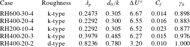
 $B=5.5$. Table 2 summarizes the parameters of the rough surfaces studied herein. It also includes the skin-friction coefficient,
 $C_{f}=2(u_{\unicode[STIX]{x1D70F}}/U_{b})^{2}$, where
 $U_{b}$ is the bulk velocity, and the contribution of drag on the hemisphere to the total drag,
 $\unicode[STIX]{x1D6FE}_{h}$. It is seen that the drag is almost entirely generated on the roughness elements and the contribution from the flat surfaces becomes progressively negligible as
 $\unicode[STIX]{x1D706}_{p}$ increases.
Parameters of the rough surfaces. Here,  $\unicode[STIX]{x1D706}_{p}$ is the plan area density defined as the ratio of projected wall-parallel area between the hemisphere and wall,
 $d_{0}$ is the zero-plane displacement,
 $\unicode[STIX]{x0394}U^{+}$ is the roughness function,
 $C_{f}=2(u_{\unicode[STIX]{x1D70F}}/U_{b})^{2}$ is the skin-friction coefficient with the bulk velocity
 $U_{b}=1$, and
 $\unicode[STIX]{x1D6FE}_{h}$ is the total drag on the hemispheres divided by the total wall shear stress.

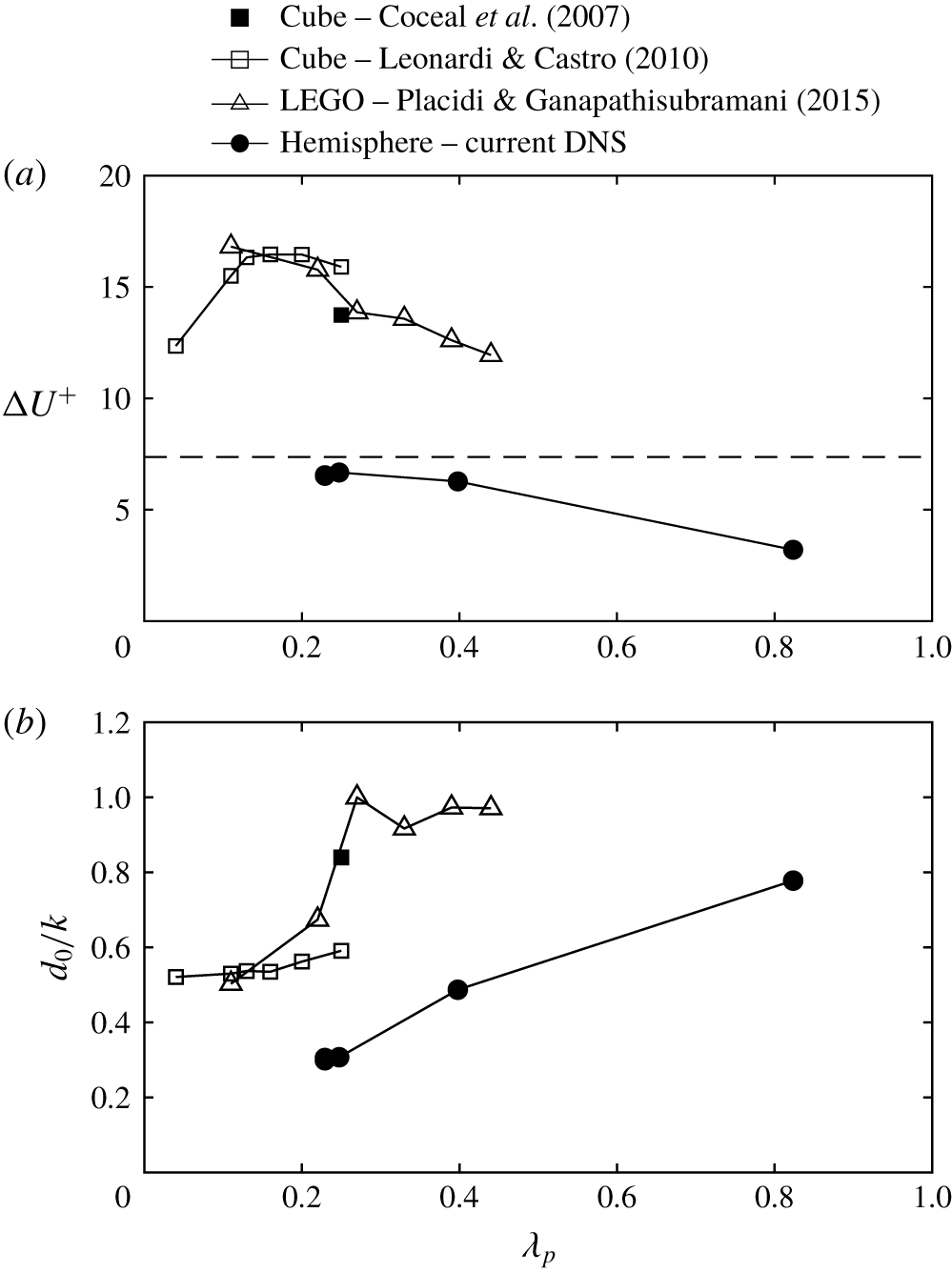
(a) Roughness function,  $\unicode[STIX]{x0394}U^{+}$, and (b) normalized zero-plane displacement,
 $d_{0}/k$, plotted as a function of the plan area density,
 $\unicode[STIX]{x1D706}_{p}$, for all rough-wall cases compared to other 3-D roughness shapes (cube and LEGO) from previous studies. The dashed line in (a) demarcates the lower limit of the fully rough regime corresponding to
 $k_{s}^{+}=70$.

Figure 3(a) compares  $\unicode[STIX]{x0394}U^{+}$ as a function of
 $\unicode[STIX]{x1D706}_{p}$ from the current DNS data with other 3-D roughness shapes from previous studies. Coceal et al. (Reference Coceal, Dobre, Thomas and Belcher2007) studied staggered arrays of cubes at
 $k^{+}\approx 500$ and reported
 $\unicode[STIX]{x0394}U^{+}\approx 13.7$ for
 $\unicode[STIX]{x1D706}_{p}=0.25$. In addition, Leonardi & Castro (Reference Leonardi and Castro2010) investigated cubic roughness elements at
 $k^{+}\approx 600$ with the plan area density in the range
 $0.04<\unicode[STIX]{x1D706}_{p}<0.25$ and showed that the largest drag is produced around
 $\unicode[STIX]{x1D706}_{p}=0.15$. However, Placidi & Ganapathisubramani (Reference Placidi and Ganapathisubramani2015) used LEGO bricks to study the effect of plan surface coverage on
 $\unicode[STIX]{x0394}U^{+}$ at fixed frontal area density
 $\unicode[STIX]{x1D706}_{f}=0.15$ (the frontal area of element divided by the unit plan area) and found a monotonically decreasing trend with the plan area density between
 $0.11$ and
 $0.44$. They argued that the different behaviour is linked to the difference in controlling the frontal area density. For cubic roughness,
 $\unicode[STIX]{x1D706}_{f}\equiv \unicode[STIX]{x1D706}_{p}$ and increasing
 $\unicode[STIX]{x1D706}_{p}$ simultaneously increases
 $\unicode[STIX]{x1D706}_{f}$, and vice versa. While it is expected that
 $\unicode[STIX]{x0394}U^{+}$ reaches a peak value around
 $\unicode[STIX]{x1D706}_{f}=0.15$ (Jiménez Reference Jiménez2004), increasing
 $\unicode[STIX]{x1D706}_{p}$ alone at fixed
 $\unicode[STIX]{x1D706}_{f}$ leads to a transition from flow passing over isolated elements (large separation) to flow skimming over densely packed elements, which progressively reduces the drag (Placidi & Ganapathisubramani Reference Placidi and Ganapathisubramani2015). For hemispherical roughness, increasing
 $\unicode[STIX]{x1D706}_{p}$ also increases
 $\unicode[STIX]{x1D706}_{f}$, but
 $\unicode[STIX]{x1D706}_{f}\neq \unicode[STIX]{x1D706}_{p}$. As hemispheres are packed closer to each other, the flow is progressively lifted upwards and the recirculation zone is disrupted until stable vortices are formed between the cavity of densely packed elements. This results in a transition from ‘k-type’ (
 $d/k=3{-}4$) to ‘d-type’ roughness (
 $d/k=2$) and a reduction of the generated drag, consistent with the paradigm envisioned by Perry et al. (Reference Perry, Schofield and Joubert1969). It should also be noted that, although
 $k^{+}=20$ is much lower compared to that used in previous studies, it is approaching the lower limit of the fully rough regime demarcated by the dashed line corresponding to
 $k_{s}^{+}=70$ for sparsely spaced roughness. The zero-plane displacement normalized by the roughness height,
 $d_{0}/k$, is shown in figure 3(b) and it is observed that
 $d_{0}/k$ increases with an increase in
 $\unicode[STIX]{x1D706}_{p}$ and it approaches
 $d_{0}=k$ at large
 $\unicode[STIX]{x1D706}_{p}$, in agreement with previous studies.
3.3 Spectral analysis
A proper spectral analysis of any field defined on an arbitrary surface requires projection on the spectrum of a Sturm–Liouville problem defined on a curvilinear manifold. The natural choice for a general periodic surface is to employ the spectrum of the Laplace–Beltrami operator on that surface. This is not a trivial spectrum for the roughness herein, which is only  ${\mathcal{C}}^{0}$ continuous; more precisely, piecewise
 ${\mathcal{C}}^{\infty }$ with discontinuity of the gradient at the contact line (the circle defined by the intersection of the hemisphere with the flat surface). Fortunately, since the pressure on the hemispherical roughness contributes heavily to the wall shear stress, it is possible to use the spherical spectrum to analyse the drag. Furthermore, pressure does not contribute to the streamwise force along the flat part of the surface, only viscous stresses do, and this contribution becomes less significant with increasing
 $Re$ and decreasing roughness separation. Therefore, we emphasize herein the spectral analysis of the wall shear stress on the hemispherical dome, and, as shown by the ratio between the total drag on the hemispheres and the total wall shear stress,
 $\unicode[STIX]{x1D6FE}_{h}$, included in table 2, and the spectra in the subsequent sections, that the ignored viscous drag on the flat sections is small.
Spherical harmonics are employed to analyse the distribution of wall shear stress on the surface of hemispheres. These harmonics arise from the solution of Laplace’s equation in spherical coordinates  $\{(r,\unicode[STIX]{x1D703},\unicode[STIX]{x1D719})\mid r\in \mathbb{R}^{+},\unicode[STIX]{x1D703}\in [0,\unicode[STIX]{x03C0}],\unicode[STIX]{x1D719}\in [0,2\unicode[STIX]{x03C0})\}$ using separation of variables. The angular part of Laplace’s equation satisfies a Sturm–Liouville problem, resulting in a complete set of orthogonal functions. These functions are traditionally referred to as spherical harmonics,
 $Y_{l}^{m}(\unicode[STIX]{x1D703},\unicode[STIX]{x1D719})$, expressed as
 $$\begin{eqnarray}Y_{l}^{m}(\unicode[STIX]{x1D703},\unicode[STIX]{x1D719})=\sqrt{\frac{(2l+1)}{4\unicode[STIX]{x03C0}}\frac{(l-m)!}{(l+m)!}}\,P_{l}^{m}(\cos \unicode[STIX]{x1D703})\text{e}^{\text{i}m\unicode[STIX]{x1D719}},\end{eqnarray}$$
for integers  $l\geqslant 0$ and
 $m$ with
 $-l\leqslant m\leqslant l$, where
 $P_{l}^{m}(\cos \unicode[STIX]{x1D703})$ are the associated Legendre polynomials of degree
 $l$ and order
 $m$ and i denotes the imaginary number. Conventionally,
 $l$ is referred to as the spherical wavenumber while
 $m$ is recognized as the Fourier wavenumber. The constant factor in (3.2) is chosen to normalize the spherical harmonics such that
 $$\begin{eqnarray}\int |Y_{l}^{m}(\unicode[STIX]{x1D703},\unicode[STIX]{x1D719})|^{2}\,\text{d}\unicode[STIX]{x1D6FA}=1,\end{eqnarray}$$
where  $\text{d}\unicode[STIX]{x1D6FA}=\sin \unicode[STIX]{x1D703}\,\text{d}\unicode[STIX]{x1D703}\,\text{d}\unicode[STIX]{x1D719}$ is the differential solid angle in spherical coordinates. The orthogonality relation is given by
 $$\begin{eqnarray}\int Y_{l}^{m}(\unicode[STIX]{x1D703},\unicode[STIX]{x1D719})\,Y_{l^{\prime }}^{m^{\prime }\ast }(\unicode[STIX]{x1D703},\unicode[STIX]{x1D719})\,\text{d}\unicode[STIX]{x1D6FA}=\unicode[STIX]{x1D6FF}_{ll^{\prime }}\unicode[STIX]{x1D6FF}_{mm^{\prime }},\end{eqnarray}$$
where  $^{\ast }$ denotes the complex conjugate. Since the spherical harmonics form a complete set of an orthonormal basis in the Hilbert space of square-integrable functions, any well-behaved functions
 $f(\unicode[STIX]{x1D703},\unicode[STIX]{x1D719})$ defined on a sphere can be represented as Laplace series, given by
 $$\begin{eqnarray}f(\unicode[STIX]{x1D703},\unicode[STIX]{x1D719})=\mathop{\sum }_{l=0}^{N_{l}}\mathop{\sum }_{m=-l}^{l}f_{lm}Y_{l}^{m}(\unicode[STIX]{x1D703},\unicode[STIX]{x1D719}),\end{eqnarray}$$
where  $N_{l}$ is the maximum degree of the spherical harmonics available due to the finite resolution of the computational mesh. The constant coefficients
 $f_{lm}$ can be readily obtained by projecting
 $f$ onto each basis function
 $Y_{l}^{m}$, according to
 $$\begin{eqnarray}f_{lm}=\int f(\unicode[STIX]{x1D703},\unicode[STIX]{x1D719})\,Y_{l}^{m\ast }(\unicode[STIX]{x1D703},\unicode[STIX]{x1D719})\,\text{d}\unicode[STIX]{x1D6FA}.\end{eqnarray}$$
Spherical harmonics can also be used to reveal the dominant modes contributing to the wall shear stress by studying the power spectrum of the coefficients. Parseval’s theorem of the spherical harmonics expansion is given by
 $$\begin{eqnarray}\Vert \,f\Vert ^{2}=\int |\,f|^{2}\,\text{d}\unicode[STIX]{x1D6FA}\approx \mathop{\sum }_{l=0}^{N_{l}}\left[\mathop{\sum }_{m=-l}^{l}|\,f_{lm}|^{2}\right]=\mathop{\sum }_{l=0}^{N_{l}}\mathscr{P}_{l}(f),\end{eqnarray}$$
where the terms in the square brackets are denoted by  $\mathscr{P}_{l}(f)$ and represent the power spectrum for spherical wavenumber
 $l$ where the Fourier modes have been summed. Furthermore, we denote the statistical average over all hemispheres by
 $$\begin{eqnarray}\langle \langle \,f\rangle \rangle =\frac{1}{N_{h}}\mathop{\sum }_{j}f^{j},\end{eqnarray}$$
where  $N_{h}$ denotes the total number of hemispheres and
 $f^{j}$ any quantity of the
 $j$th hemisphere. We assume that this ensemble average is reasonably well converged given the large number of hemispheres present in the DNS (see table 1). The smallest case investigated herein, RH200-10-4, has
 $2304$ hemispheres, yielding a statistical error of
 $1/\sqrt{2304}\sim 2\,\%$, which drops to
 ${\sim}0.5\,\%$ for the largest case, RH400-20-2, with
 $33\,120$ hemispheres. This requirement highlights the need to devise the use of such a large number of roughness elements.
Though the rough surfaces studied herein are composed of hemispheres, the framework of spherical harmonics is still applicable by assuming that  $f$ is an even function about the equator of a sphere, where the function on the upper hemisphere is mirrored to the lower half. This works exactly for the pressure because flow smoothness near the contact line requires the radial derivative of pressure to vanish, something that is less clear for the viscous stresses. In this way, the spherical harmonics coefficients can be computed directly from the simulations by integrating a given function with the complex conjugate of the basis functions defined on the surface of each hemisphere using the Gauss–Lobatto quadrature rule, i.e. (3.6). The maximum degree is determined by the accuracy of the surface mesh used in the simulation, which is
 $N_{l}=6$ for the resolutions used in the DNS (see
 $M_{h}$ in table 1). Once all available coefficients are obtained, any function can be reconstructed using (3.5). In contrast to smooth-wall flows, where wall shear stress is solely determined by viscous stresses, rough-wall flow also induces pressure drag, which dominates at sufficiently high
 $Re$ when the flow approaches fully rough conditions (Raupach et al. Reference Raupach, Antonia and Rajagopalan1991; Jiménez Reference Jiménez2004; Flack & Schultz Reference Flack and Schultz2010). For completeness, we analyse both pressure and viscous contributions projected along the streamwise direction, denoting
 $p_{x}=-pn_{x}$ and
 $\unicode[STIX]{x1D70E}_{x}=[\unicode[STIX]{x1D748}\boldsymbol{\cdot }\boldsymbol{n}]_{x}$, respectively, where
 $\boldsymbol{n}=\{n_{x},n_{y},n_{z}\}$ is the unit outward normal vector of the surface and
 $\unicode[STIX]{x1D748}=\unicode[STIX]{x1D707}(\unicode[STIX]{x1D6FB}\boldsymbol{u}+\unicode[STIX]{x1D6FB}\boldsymbol{u}^{\text{T}})$ is the viscous part of the stress tensor. Obviously, the sum of the pressure and viscous contributions represents the total wall shear stress along the streamwise direction, i.e.
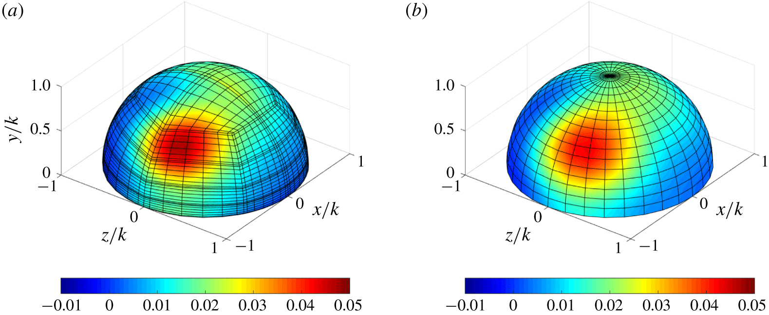
 $\unicode[STIX]{x1D70F}_{x}=p_{x}+\unicode[STIX]{x1D70E}_{x}$. A comparison of the original (simulation) and spectrally reconstructed instantaneous wall shear stress on an arbitrarily chosen hemisphere is shown in figure 4 for simulation RH400-20-4. It can be seen that the spectrally reconstructed field is very close to the original field, as it should be, and most features are well captured, although note that the mesh used to reconstruct the flow field is not the same as the simulation mesh since spherical harmonics are invariant to the choice of grid points.
Example of the instantaneous wall shear stress  $\unicode[STIX]{x1D70F}_{x}$ on an arbitrary hemisphere for RH400-20-4. (a) Actual field extracted from DNS and (b) reconstructed field using spherical harmonics.

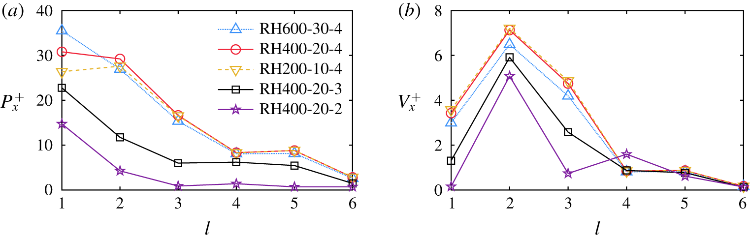
Power spectrum of the spherical harmonic expansion as a function of the spherical wavenumber  $l$ over various rough surfaces for the streamwise-projected (a) pressure
 $P_{x}^{+}$ and (b) viscous stress
 $V_{x}^{+}$, respectively. Note that the power spectrum is averaged over all hemispheres and normalized by the friction velocity
 $u_{\unicode[STIX]{x1D70F}}$.

Figure 5 shows the power spectra for the streamwise-projected pressure,  $P_{x}^{+}=\langle \langle \mathscr{P}_{l}(p_{x})\rangle \rangle ^{+}$, and viscous stress,
 $V_{x}^{+}=\langle \langle \mathscr{P}_{l}(\unicode[STIX]{x1D70E}_{x})\rangle \rangle ^{+}$, averaged over all hemispheres. Note that
 $(\cdot )^{+}$ denotes normalization by the friction velocity
 $u_{\unicode[STIX]{x1D70F}}$. As shown in figure 5(a),
 $P_{x}^{+}$ scales well with
 $Re$ for all roughness cases with the same element separation
 $d/k=4$, except for mode
 $l=1$ in which the energy content increases slightly with
 $Re$. However, as the element spacing is decreased, the pressure contribution to the overall wall shear stress decreases. In addition, it is seen that
 $P_{x}^{+}$ peaks at low wavemodes and decays rapidly as wavenumber increases.
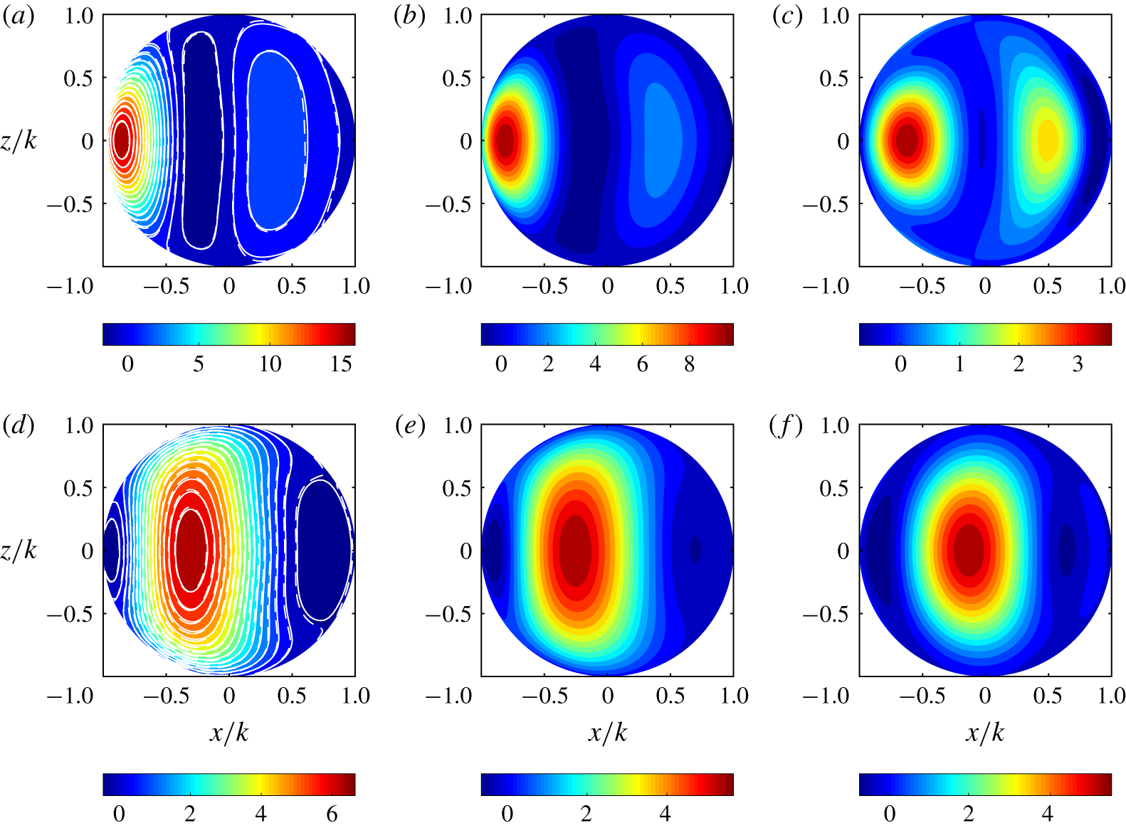
Contours of the streamwise-projected (a–c) pressure,  $\langle \langle p_{x}\rangle \rangle ^{+}$, and (d–f) viscous stress,
 $\langle \langle \unicode[STIX]{x1D70E}_{x}\rangle \rangle ^{+}$, for (a,d)
 $d/k=4$, (b,e)
 $d/k=3$ and (c,f)
 $d/k=2$. The colour map is plotted for cases at
 $Re_{\unicode[STIX]{x1D70F}}=400$. Solid and dashed contour lines are superimposed in (a) and (d) for cases at
 $Re_{\unicode[STIX]{x1D70F}}=600$ and
 $200$, respectively.

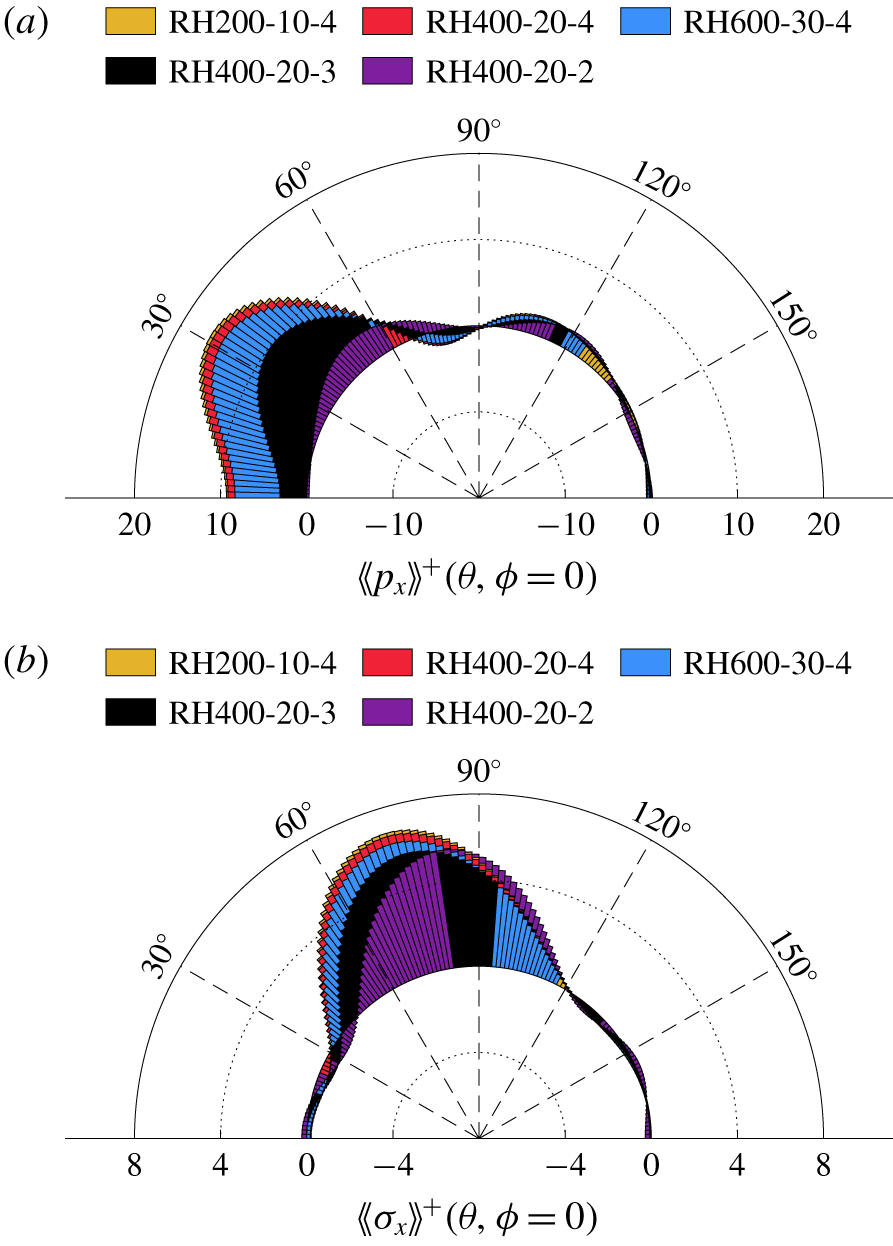
Distribution of streamwise-projected (a) pressure and (b) viscous stress along the centre meridian.

This behaviour is demonstrated graphically by plotting the surface distribution of  $\langle \langle p_{x}\rangle \rangle ^{+}$, reconstructed using spherical harmonics and shown in figure 6(a–c) for all rough-wall cases. Note that, when averaging over all hemispheres to determine this quantity, one must delete
 $p_{00}$ because each hemisphere experiences a slightly different uniform pressure level that does not contribute to the overall drag. The spurious
 $-\langle \langle p_{00}\rangle \rangle n_{x}\neq 0$ has no physical relevance and evidently the average of this mode over the surface of the hemisphere is exactly zero. It is readily seen that the average distribution is symmetric about the spanwise mid-plane for each case. A region of high streamwise-projected pressure
 $\langle \langle p_{x}\rangle \rangle ^{+}$ is observed on the windward side of the hemisphere, corresponding to the flow stagnation point; the exact location of the peak
 $\langle \langle p_{x}\rangle \rangle ^{+}$ varies with the element pitch-to-height ratio,
 $d/k$. More interestingly, a relatively high
 $\langle \langle p_{x}\rangle \rangle ^{+}$ zone is observed in the region of fluid suction on the leeward side of the hemisphere, which becomes more prominent for the closely packed hemisphere arrangement (RH400-20-2). Results from
 $Re_{\unicode[STIX]{x1D70F}}=600$ and
 $200$ are also superimposed as solid and dashed contour lines, respectively, in figure 6(a). It is observed that the distribution is insensitive to the
 $Re$ effect, as expected, since the friction roughness height
 $k^{+}=20$ is kept constant in all cases.
Figure 7(a) shows the distribution of  $\langle \langle p_{x}\rangle \rangle ^{+}$ along the centre meridian for the all rough walls. When the hemispheres are far apart (
 $d/k=4$), the maximum of
 $\langle \langle p_{x}\rangle \rangle ^{+}$ occurs near
 $30^{\circ }$, whereas the minimum is located around
 $80^{\circ }$. As the element separation decreases (
 $d/k=3$), the peak value of
 $\langle \langle p_{x}\rangle \rangle ^{+}$ drops whereas the peak location ascends gradually towards the apex of the hemisphere. The overall pressure difference across the hemisphere also decreases with decreasing
 $d/k$, owing to fluid being lifted away from the wall, resulting in reduced flow momentum within the roughness sublayer. The trends of packing density continues for the closely packed hemispheres (
 $d/k=2$), where the peak projected pressure stress drops further and the location reaches approximately
 $60^{\circ }$. On the leeward side, the high-pressure region now becomes as strong as on the windward side, both being the major flow features for this roughness configuration. Similar behaviour has also been observed previously for cubic roughness, where recirculation regions between denser arrays of cubes become the predominant inter-cube flow feature, which can even generate a negative contribution to the total drag (Leonardi & Castro Reference Leonardi and Castro2010). However, the contribution to drag is always positive in the cases studied herein.
While a similar trend is observed for the streamwise-projected viscous stress,  $V_{x}^{+}$, as shown in figure 5(b), it appears that the dominant mode is the second spherical harmonic mode, i.e.
 $l=2$, and the energy of this mode increases slightly with increasing element spacing. This observation is consistent with the graphical representations shown in figure 6(d–f), where the predominant feature is the bulk high-stress region centred around
 $70^{\circ }$–
 $80^{\circ }$ on the windward side of the hemisphere. In addition, it is shown that the energy contained in the spherical modes
 $l=1$ and
 $3$ is also strongly influenced by the element spacing. Based on the characteristic length scales of the vortical structures, the spherical mode
 $l=1$ corresponds to coherent structures that are consistently seen within the roughness sublayer and cover the windward area of the hemisphere owing to the generation of surface vorticity lines, whereas the horseshoe vortices developed by the concentration of vorticity loops upstream of hemispheres are associated with the spherical mode
 $l=3$. As the element spacing decreases, the pressure gradient across the hemispheres is reduced. Consequently, the strength of surface vorticity is weakened, in agreement with the decrease of peak
 $\langle \langle \unicode[STIX]{x1D70E}_{x}\rangle \rangle ^{+}$ shown in figure 7(b), whereas the rollup of vorticity loops near the base of hemispheres is inhibited in the denser arrays of roughness elements, which is readily seen in figure 6(d–f), where the shrinkage of high-stress regions commences near the frontal edge of the hemisphere. Therefore, the energy stored in modes
 $l=1$ and
 $3$ drops dramatically as the roughness elements become closer to one another.
3.4 Roughness-cell-averaged statistics
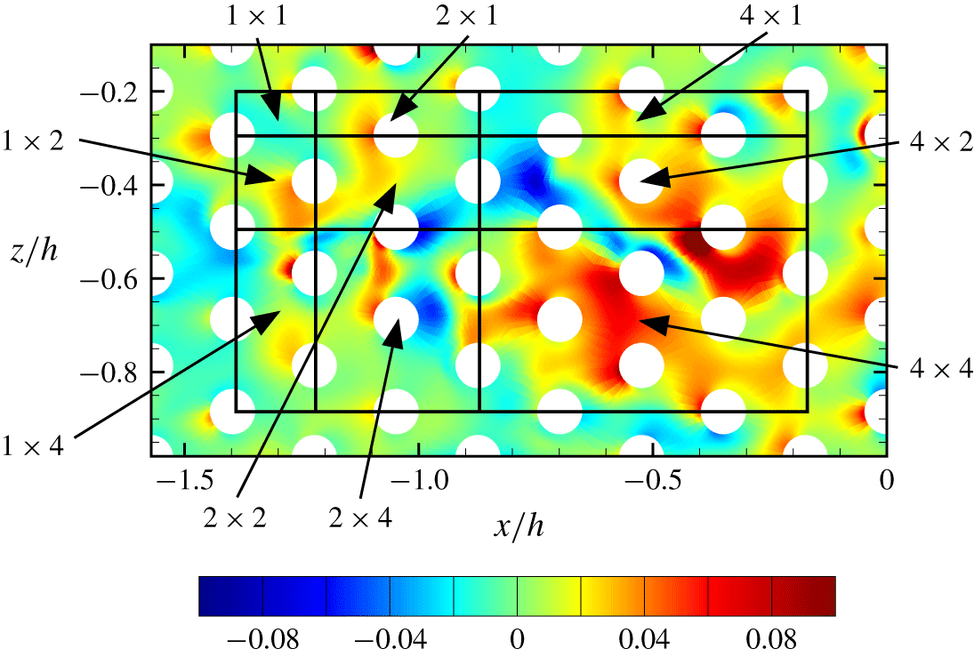
From the point of view of multiscale modelling, i.e. LES, the most detailed information one expects to use in turbulence wall models is the mean wall shear stress. With the presence of roughness elements, the time-averaged statistics are not spatially homogeneous at wall-parallel planes within the roughness sublayer. However, planar averaging over a repeating unit of a uniform array, which has been used by Raupach et al. (Reference Raupach, Antonia and Rajagopalan1991) and Cheng & Castro (Reference Cheng and Castro2002), can lead to a quantitative representation of the roughness sublayer that can be regarded as spatially homogeneous on scales larger than the unit size. Similarly, Hong, Katz & Schultz (Reference Hong, Katz and Schultz2011) performed conditional spatial averaging within a square region to investigate the spatial variations of statistics for uniformly packed pyramidal roughness. In analogy, before further analysis can be carried out, we define the minimal unit of surface over which the wall shear stress is integrated, and refer to it as a ‘roughness unit cell’ or ‘minimal cell’. This surface contains a quarter of the hemisphere on the leeward side and a quarter on the windward side. Note that, because of the symmetry of each roughness element, the minimal cell is half of what would be expected, since the flow is mirrored on the symmetric side, in a statistical sense. An entire rough wall can then be partitioned into arrays of minimal cells in both streamwise and spanwise directions. Figure 8 shows a sketch of the minimal cell denoted as the ‘ $1\times 1$’ cell. Note that one may choose different unit-cell configurations from those shown, but it is reasonable to perform surface integration of the wall shear stress over cells that contain both windward and leeward portions of the roughness, therefore taking into account the physics involved on both sides. For simplicity, a box is chosen as the basic cell configuration for the conditional spatial average, but hexagonal polygons could also be used in this hemisphere arrangement. Larger cells are constructed by repeating integer multiples of the fundamental roughness cell along the streamwise and spanwise directions. In the nomenclature introduced here, the first number corresponds to the extent in the streamwise direction while the second number denotes the extent in the spanwise direction. If one assembles the mean wall shear stress as an array of values, they form a homogeneous and periodic sequence that is amenable to spectral analysis, as is regularly used in the study of smooth-wall statistics when using pointwise values of the wall shear stress.
Roughness cell nomenclature and instantaneous pressure  $p$ for RH400-20-4 at
 $y^{+}=5$.

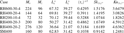
Minimal roughness-cell-averaged statistics of wall shear stress.  $M_{x}{-}M_{z}$ represent the number of cells sampled in the streamwise and spanwise, respectively, with the corresponding dimensions,
 $L_{x}^{+}{-}L_{z}^{+}$ in wall units. The variance, skewness and kurtosis (subtracted by 3) of the wall shear stress are also included.

Therefore, the instantaneous pressure and viscous stresses were integrated over the rough minimal cell of surface  $S$ with the outward normal vector
 $\boldsymbol{n}=\{n_{x},n_{y},n_{z}\}$ and averaged by the projected horizontal flat surface area
 $A_{f}$, yielding the cell-averaged streamwise wall shear stress
 $\langle \unicode[STIX]{x1D70F}_{x}\rangle$, given by
 $$\begin{eqnarray}\langle \unicode[STIX]{x1D70F}_{x}\rangle (\boldsymbol{m})=\frac{1}{A_{f}}\int _{\unicode[STIX]{x1D6FA}}[\unicode[STIX]{x1D749}\boldsymbol{\cdot }\boldsymbol{n}]_{x}(x,y,z)\,\text{d}S=\langle p_{x}\rangle (\boldsymbol{m})+\langle \unicode[STIX]{x1D70E}_{x}\rangle (\boldsymbol{m}),\end{eqnarray}$$
where  $\unicode[STIX]{x1D749}$ is the Newtonian stress tensor,
 $\langle p_{x}\rangle$ and
 $\langle \unicode[STIX]{x1D70E}_{x}\rangle$ are the corresponding cell-averaged pressure and viscous components, respectively, and the angle brackets denote the cell average. The two-index
 $\boldsymbol{m}=(m_{x},m_{z})$ with
 $m_{x}\in [0,M_{x}{-}1]$ and
 $m_{z}\in [0,M_{z}{-}1]$ denotes the discrete indices along the streamwise and spanwise directions with repeated cells
 $M_{x}{-}M_{z}$, respectively, and the corresponding dimensions,
 $L_{x}^{+}{-}L_{z}^{+}$. Table 3 summarizes the computation parameters for the minimal cell for each roughness case. For convenience, the horizontal coordinates are denoted discretely by
 $(x,z)=(Lm_{x}/M_{x},Wm_{z}/M_{z})$. Note that averaging all of the cell-averaged streamwise wall shear stresses equates to the mean wall shear stress
 $\bar{\unicode[STIX]{x1D70F}}_{w}$. For better convergence of the statistics, cell-averaged statistics for each roughness case are also collected in time over a total time
 $T^{+}=Tu_{\unicode[STIX]{x1D70F}}/h\approx 10$. The variance, skewness and kurtosis (subtracted by 3) for the wall shear stress are included as well. The statistics for the smooth-wall flow are also reported for comparison purposes.
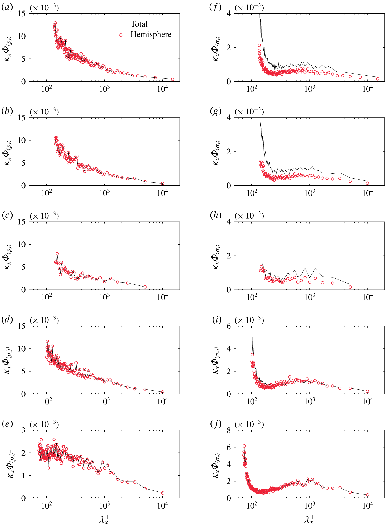
Pre-multiplied 1-D streamwise spectra of the roughness-cell-averaged (a–e) pressure and (f–j) viscous stress projected in the streamwise direction, averaged with the minimal cell ‘ $1\times 1$’ for (a,f) RH600-30-4, (b,g) RH400-20-4, (c,h) RH200-10-4, (d,i) RH400-20-3 and (e,j) RH400-20-2. See panel (a) for key.

Figure 9 compares pre-multiplied one-dimensional (1-D) streamwise spectra of the roughness-cell-averaged pressure and viscous stress contributions for all rough-wall cases. The power spectra for the pressure contribution,  $\unicode[STIX]{x1D6F7}_{\langle p_{x}\rangle }(\unicode[STIX]{x1D705}_{x})=\widehat{\langle p_{x}\rangle }\widehat{\langle p_{x}\rangle }^{\ast }(\unicode[STIX]{x1D705}_{x})$, as a function of the discrete streamwise wavenumber
 $\unicode[STIX]{x1D705}_{x}=2\unicode[STIX]{x03C0}j/L$ for
 $j=-M_{x}/2+1,\ldots ,0,1,\ldots ,M_{x}/2$, are calculated from the spatial series with the minimal-cell-averaged Fourier coefficients
 $\widehat{\langle p_{x}\rangle }(\unicode[STIX]{x1D705}_{x})$. The same approach was applied to the viscous contribution. Each panel in figure 9 shows two curves, one (solid lines) using the total wall shear stress from integration of the forces over all surfaces (termed ‘total’) and a second curve (circles) that considers only the hemisphere part of each roughness cell (termed ‘hemisphere’). The pressure contribution shown in figure 9(a–e) is identical in both curves since pressure only contributes to the drag over the hemispherical dome. However, the curves for the viscous contribution, as shown in figure 9(f–j), differ because the drag over the flat horizontal surface is ignored in the latter case. This difference reduces with decreasing element spacing, from top to bottom, since the viscous stress is dominantly produced on the hemisphere surface and the contribution from the flat surface progressively diminishes. It should be noted that the pressure is still the largest contributor to the overall drag (note differences in the vertical scale range), as expected. Furthermore, the spectra of the viscous stress contribution are shown to have an inner peak corresponding to the intrinsic shedding off the roughness elements and an outer (centre) peak associated with the most energetic near-wall streaky structures. It is also worth noting that the energy contained in scales smaller than the minimal cell size is manifested in the spectra as aliased energy at the smallest scale captured by the minimal cell size. Since the size of the minimal cell is controlled by the geometry of the roughness topography, it is expected that the aliased energy is relatively smaller for the closely packed hemispheres as the spectra roll off at smaller scales (corresponding to the streamwise extent of the minimal cell). This comparison is carried out to show that the spherical harmonics analysis of the drag contributions over the hemisphere discussed in § 3.3 reproduce well the spectra of the wall shear stress when the roughness spacing is small. However, even for larger element spacing, the viscous contributions to the drag are substantially less than that of the pressure, confirming that most of the relevant drag is produced by the roughness elements, one way or the other (Raupach et al. Reference Raupach, Antonia and Rajagopalan1991).
The main difference between the pressure and viscous power spectra, qualitatively speaking, is the large peak observed near the cutoff scale (left-hand side) of the wavelength range. This occurs because all contributions of smaller scales than the size of the minimal cell, i.e. flow within the roughness element, is aliased to higher wavelengths, and most predominantly to the energy around the cutoff scale. It is reasonable to conclude that a substantial part of the viscous contribution comes from the small-scale dynamics within the roughness cell, as opposed to large-scale, inter-roughness viscous effects.
4 Wall shear stress from the perspective of amplitude modulation
The statistical behaviour of the wall shear stress is useful in the modelling of wall-bounded turbulent flows where the effects of the inner layer are modelled rather than fully resolved. Practical LES, i.e. wall unresolved, employs computational grid spacings that are much larger than the size of the minimal roughness cell. Thus, it is highly relevant to investigate the statistical properties of the averaged wall shear stress over surfaces that include multiple roughness elements in order to ensure that the results presented herein have practical impact on improved LES modelling.
As shown in figure 8, averaging surfaces that are integer multiples of the minimal cell are considered, labelled by the corresponding two numbers that denote their streamwise and spanwise extent with respect to the minimal cell, respectively. However, before describing the detailed statistics of the averaged wall shear stress, it is recognized that previous experiments in smooth-wall TBLs at high  $Re$ have shown that the near-wall small scales are amplitude-modulated by outer-layer, large-scale structures (Mathis et al. Reference Mathis, Hutchins and Marusic2009, Reference Mathis, Hutchins and Marusic2011; Marusic, Mathis & Hutchins Reference Marusic, Mathis and Hutchins2010). More recently, several experimental and numerical studies (Nadeem et al. Reference Nadeem, Lee, Lee and Sung2015; Anderson Reference Anderson2016; Squire et al. Reference Squire, Baars, Hutchins and Marusic2016; Pathikonda & Christensen Reference Pathikonda and Christensen2017) have also demonstrated the occurrence of AM effects in wall-bounded turbulent flows exposed to rough walls. These studies highlight the importance of inner–outer interactions where the large scales that reside in the inertial region of the boundary layer affect the near-wall flow dynamics regardless of the wall condition (smooth or rough). Mathis et al. (Reference Mathis, Marusic, Chernyshenko and Hutchins2013) identified a similar AM paradigm between the large scales in the outer layer and the wall shear stress and proposed a model for predicting statistics of the latter based on knowledge of the former. The analysis of the wall shear stress from this perspective is desirable because one can isolate purely statistical behaviour of the wall shear stress, excluding the local and instantaneous modulations induced by the larger scales in the outer layer. This leads to somewhat more universal information that is not polluted by large-scale effects.
Therefore, we concentrate on fluctuations of the cell-averaged streamwise wall shear stress  $\langle \unicode[STIX]{x1D70F}_{x}\rangle ^{\prime +}$, which can be further decomposed into large-scale and small-scale components, according to (
 $m_{z}$ is omitted for brevity)
 $$\begin{eqnarray}\langle \unicode[STIX]{x1D70F}_{x}\rangle ^{\prime +}(m_{x})=\langle \unicode[STIX]{x1D70F}_{x}\rangle _{{\mathcal{L}}}^{\prime +}(m_{x})+\langle \unicode[STIX]{x1D70F}_{x}\rangle _{{\mathcal{S}}}^{\prime +}(m_{x}),\end{eqnarray}$$
where the large-scale component is obtained by filtering  $\langle \unicode[STIX]{x1D70F}_{x}\rangle ^{\prime +}(m_{x})$ with a sharp spectral filter with cutoff wavenumber
 $\unicode[STIX]{x1D705}_{c}$, yielding
 $$\begin{eqnarray}\langle \unicode[STIX]{x1D70F}_{x}\rangle _{{\mathcal{L}}}^{\prime +}(m_{x})\equiv \mathop{\sum }_{\unicode[STIX]{x1D705}_{x}}H(\unicode[STIX]{x1D705}_{c}-|\unicode[STIX]{x1D705}_{x}|)\widehat{\langle \unicode[STIX]{x1D70F}_{x}\rangle }^{\prime +}(\unicode[STIX]{x1D705}_{x})\text{e}^{\text{i}\unicode[STIX]{x1D705}_{x}m_{x}L/M_{x}},\end{eqnarray}$$
where  $H$ is the Heaviside function and the cutoff wavenumber is chosen to be
 $\unicode[STIX]{x1D705}_{c}=\unicode[STIX]{x03C0}/h$, which corresponds to the integral length scale, the half-channel height
 $h$, and
 $\widehat{\langle \unicode[STIX]{x1D70F}_{x}\rangle }$ denotes the Fourier coefficients of
 $\langle \unicode[STIX]{x1D70F}_{x}\rangle$. Then, the Hilbert transform is applied to the small-scale component of the cell-averaged wall shear stress to extract the envelope of the signal, which is then filtered again at
 $\unicode[STIX]{x1D705}_{c}$ to remove the remaining small-scale effects, yielding the large-scale component of the envelope of the small-scale cell-averaged wall shear stress,
 $E_{{\mathcal{L}}}\{\langle \unicode[STIX]{x1D70F}_{x}\rangle _{{\mathcal{S}}}^{\prime +}(m_{x})\}$. More in-depth details on this decomposition process can be found in Mathis et al. (Reference Mathis, Hutchins and Marusic2011, Reference Mathis, Marusic, Chernyshenko and Hutchins2013).
4.1 Two-point AM correlation coefficients
Similar to the two-point AM correlation coefficient defined originally by Mathis et al. (Reference Mathis, Hutchins and Marusic2009) based on outer- and inner-layer velocity signals, the correlation between the filtered envelope of the small-scale, cell-averaged streamwise wall shear stress  $E_{{\mathcal{L}}}\{\langle \unicode[STIX]{x1D70F}_{x}\rangle _{{\mathcal{S}}}^{\prime +}\}$ and the large-scale, cell-averaged streamwise velocity signal
 $\langle u\rangle _{{\mathcal{L}}}^{\prime +}$ at any given
 $y$ in the outer layer is given by
 $$\begin{eqnarray}R_{wall}(y)=\frac{\overline{\langle u\rangle _{{\mathcal{L}}}^{\prime +}(y)E_{{\mathcal{L}}}\{\langle \unicode[STIX]{x1D70F}_{x}\rangle _{{\mathcal{S}}}^{\prime +}\}}}{\sqrt{\overline{\langle u\rangle _{{\mathcal{L}}}^{\prime +}(y)^{2}}}\sqrt{\overline{E_{{\mathcal{L}}}{\{\langle \unicode[STIX]{x1D70F}_{x}\rangle _{{\mathcal{S}}}^{\prime +}\}}^{2}}}}.\end{eqnarray}$$
Note that the correlation is computed along the streamwise direction at each spanwise position and then averaged in the span for the minimal-cell-averaged wall shear stress fluctuations.
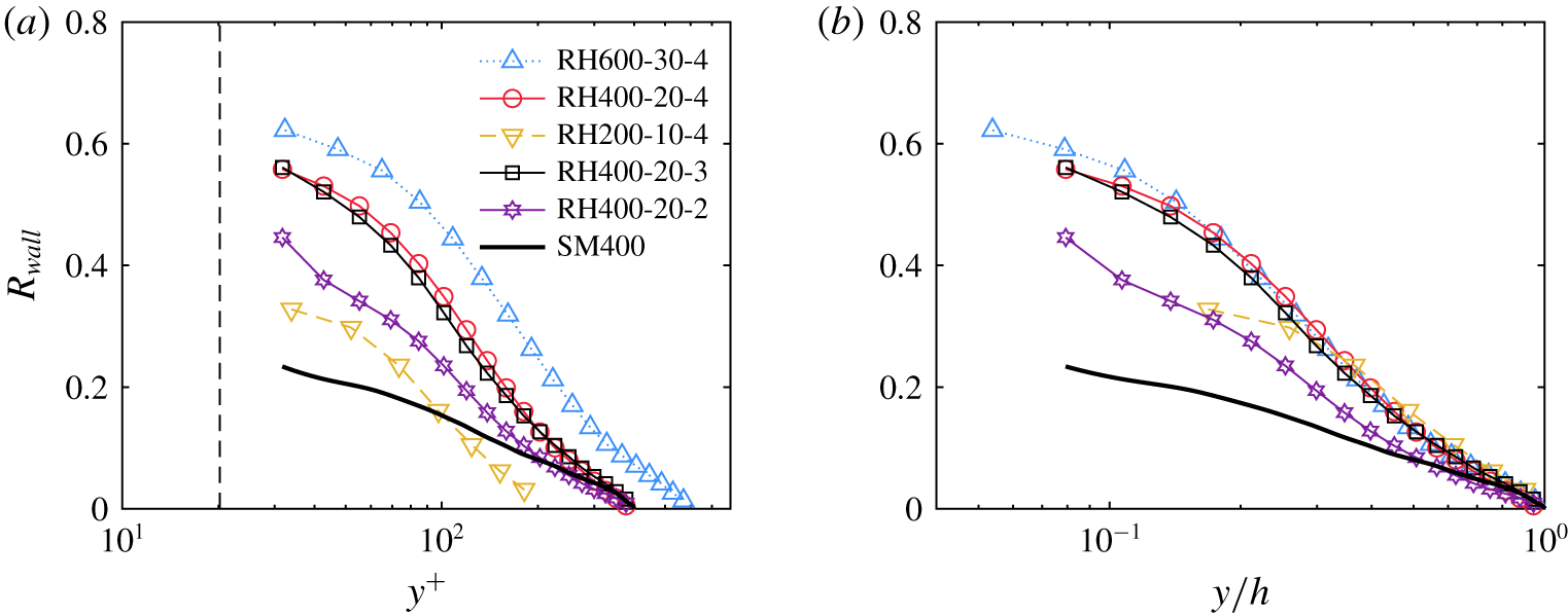
Two-point AM correlation coefficients averaged for smooth-wall and rough-wall flows with cell size ‘ $1\times 1$’ plotted as a function of the (a) inner coordinate,
 $y^{+}$, and (b) outer coordinate,
 $y/h$. The dashed vertical line in (a) denotes the roughness crest
 $k^{+}=20$.

Figure 10(a) shows the evolution of the two-point AM correlation coefficients,  $R_{wall}$, as a function of the inner wall-normal coordinate,
 $y^{+}$, for all roughness cases. Comparing the
 $Re_{\unicode[STIX]{x1D70F}}=400$ cases, it is found that roughness enhances this correlation compared to the smooth-wall result, likely because roughness tends to enhance the small-scale activities within the roughness sublayer. This behaviour is consistent with previous rough-wall studies that leveraged inner- and outer-layer velocity signals to compute the AM correlation coefficient for rough-wall flows (Nadeem et al. Reference Nadeem, Lee, Lee and Sung2015; Anderson Reference Anderson2016; Squire et al. Reference Squire, Baars, Hutchins and Marusic2016; Pathikonda & Christensen Reference Pathikonda and Christensen2017). It is also noted that, when the roughness elements are far apart (RH400-20-3 and RH400-20-4), the AM correlations are found to be even stronger than when the roughness elements are closely packed (RH400-20-2). In addition, when scaling the wall-normal coordinate by the outer length scale
 $h$ instead, as shown in figure 10(b), it is clearly seen that the AM correlation coefficients collapse very well for cases with larger element separations (
 $d/k=3{-}4$), in contrast to the case with closely packed elements (
 $d/k=2$). This suggests that the large-scale structures residing in the outer layer act differently on the near-wall turbulence for ‘k-type’ and ‘d-type’ roughness. Furthermore, although an enhanced AM of the wall shear stress is noted with increasing
 $Re$, in agreement with the trends reported by Mathis et al. (Reference Mathis, Hutchins and Marusic2009), the
 $Re$ dependence becomes rather weak between cases at
 $Re_{\unicode[STIX]{x1D70F}}=400$ and
 $600$.
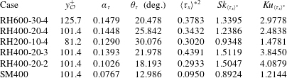
Calibration parameters for the smooth and rough walls with respect to  $y_{{\mathcal{O}}}^{+}$. The variance, skewness and kurtosis (subtracted by 3) of the universal wall shear stress are also included in the table.

4.2 Cell-averaged wall shear stress model
In a series of experimental studies of high- $Re$ smooth-wall TBLs, Mathis et al. (Reference Mathis, Hutchins and Marusic2009, Reference Mathis, Hutchins and Marusic2011) proposed and tested a robust model based on AM analysis to successfully predict near-wall fluctuating streamwise velocity statistics using only large-scale streamwise velocity signals sampled in the outer layer. Later, Mathis et al. (Reference Mathis, Marusic, Chernyshenko and Hutchins2013) extended this modelling framework to the streamwise wall shear stress based on the linear relationship with the streamwise velocity component in the viscous sublayer for smooth walls. Following Mathis et al. (Reference Mathis, Marusic, Chernyshenko and Hutchins2013), this model is adapted herein and applied to the cell-averaged streamwise wall shear stress obtained for the present roughness cases. This model can be expressed as
 $$\begin{eqnarray}\langle \unicode[STIX]{x1D70F}_{x}\rangle _{p}^{\prime +}=\langle \unicode[STIX]{x1D70F}_{x}\rangle ^{\ast }\{1+\unicode[STIX]{x1D6FC}_{\unicode[STIX]{x1D70F}}\langle u\rangle _{{\mathcal{O}}{\mathcal{L}}}^{\prime +}\}+\unicode[STIX]{x1D6FC}_{\unicode[STIX]{x1D70F}}\langle u\rangle _{{\mathcal{O}}{\mathcal{L}}}^{\prime +},\end{eqnarray}$$
where  $\langle \unicode[STIX]{x1D70F}_{x}\rangle _{p}^{\prime +}$ is the predicted streamwise wall shear stress fluctuation and
 $\langle \unicode[STIX]{x1D70F}_{x}\rangle ^{\ast }$ is the universal wall shear stress signal representing the small-scale wall shear stress fluctuation without the influence from outer LSMs. The universal signal is determined in a calibration process together with the parameters
 $\unicode[STIX]{x1D6FC}_{\unicode[STIX]{x1D70F}}$ and
 $\unicode[STIX]{x1D703}_{\unicode[STIX]{x1D70F}}$ used to account for the maximum cross-correlation and the turbulent structure angle between the fluctuating streamwise wall shear stress
 $\langle \unicode[STIX]{x1D70F}_{x}\rangle _{c}^{\prime +}$ used for calibration and the large-scale streamwise velocity in the log region
 $\langle u\rangle _{{\mathcal{O}}{\mathcal{L}}}^{\prime +}$, evaluated at
 $(x,y)=(L_{x}m_{x}+y_{{\mathcal{O}}}\cot (\unicode[STIX]{x1D703}_{\unicode[STIX]{x1D70F}}),y_{{\mathcal{O}}})$, respectively. The calibration parameters for all flow conditions are shown in table 4, along with the variance, skewness and kurtosis (subtracted by 3) of the universal wall shear stress. The smooth-wall case yields a superposition coefficient of
 $\unicode[STIX]{x1D6FC}_{\unicode[STIX]{x1D70F}}=0.0767$ and an inclination angle of
 $\unicode[STIX]{x1D703}_{\unicode[STIX]{x1D70F}}\approx 13^{\circ }$, which compare reasonably well with the values obtained in the high-
 $Re$ smooth-wall TBL experiments by Mathis et al. (Reference Mathis, Marusic, Chernyshenko and Hutchins2013), who reported
 $\unicode[STIX]{x1D6FC}=0.0898$ and
 $\unicode[STIX]{x1D703}_{L}=14.1^{\circ }$, respectively. With the presence of roughness, both
 $\unicode[STIX]{x1D6FC}_{\unicode[STIX]{x1D70F}}$ and
 $\unicode[STIX]{x1D703}_{\unicode[STIX]{x1D70F}}$ are substantially enhanced compared to smooth-wall flow; though sensitive to the roughness element spacing, the increase in these coefficients is in accordance with the investigations by Perry, Lim & Henbest (Reference Perry, Lim and Henbest1987) and Krogstad & Antonia (Reference Krogstad and Antonia1994), who reported shorter streamwise length scales and larger inclination of coherent structures in rough-wall flow as inferred from two-point velocity correlations. Ideally,
 $\langle \unicode[STIX]{x1D70F}_{x}\rangle ^{\ast }$,
 $\unicode[STIX]{x1D6FC}_{\unicode[STIX]{x1D70F}}$ and
 $\unicode[STIX]{x1D703}_{\unicode[STIX]{x1D70F}}$ documented in table 4 should be
 $Re$-independent and can be assumed universal across different types of wall-bounded turbulent flows. In practice, however, roughness likely introduces variations at scales approximately equal to the characteristic roughness scales. Subsequent discussions are devoted to the statistical behaviours of the universal wall shear stress in response to
 $Re$, roughness packing density and various spatial averaging cells.
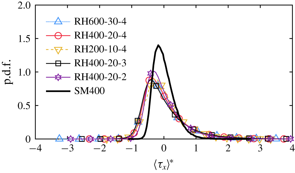
Probability density functions of the universal streamwise wall shear stress averaged with the minimal cell ‘ $1\times 1$’ for all roughness cases and the smooth-wall baseline.

The probability density functions (p.d.f.s) of the universal wall shear stress averaged over the minimal cell ‘ $1\times 1$’ for the smooth- and rough-wall flows are shown in figure 11. It is observed that the p.d.f. of
 $\langle \unicode[STIX]{x1D70F}_{x}\rangle ^{\ast }$ is wider and more skewed towards weaker stress values in rough-wall flow compared to smooth-wall flow. The probability of high and low extreme events is also larger within the roughness sublayer, indicating more intermittent regions due to the presence of the roughness elements. These results are well supported by the corresponding statistical properties shown in table 4. The variance, skewness and kurtosis (subtracted by 3) are larger in the roughness cases compared to those of the smooth-wall baseline.
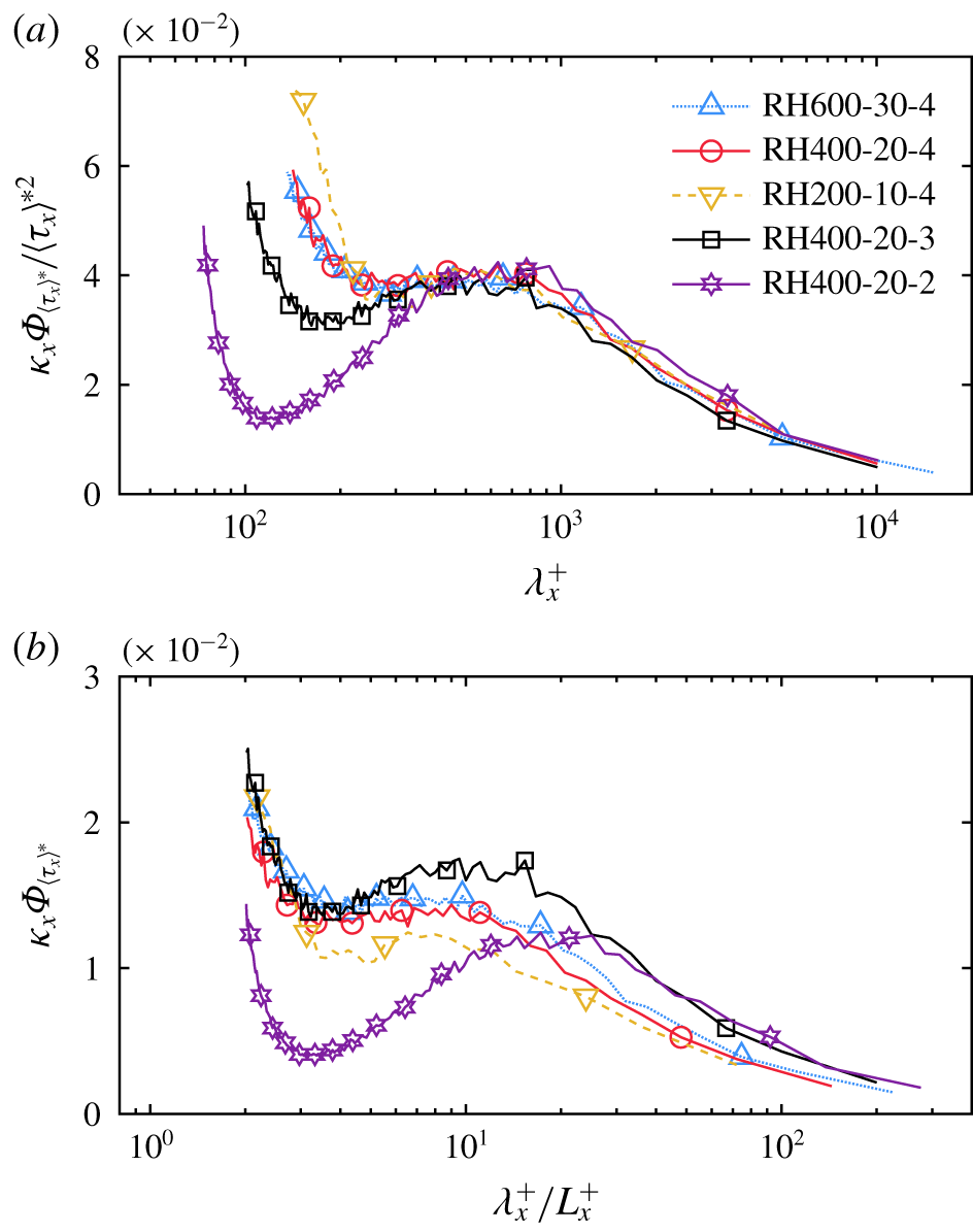
Pre-multiplied streamwise spectra of the universal wall shear stress averaged with the minimal cell ‘ $1\times 1$’ for all rough-wall flows. Note that the spectra in (a) are scaled by the stress variance
 $\langle \unicode[STIX]{x1D70F}_{x}\rangle ^{\ast 2}$ and the streamwise wavelength in (b) is scaled by the minimal cell length
 $L_{x}^{+}$ (leaving the spectra in inner units).

While figure 11 indicates reasonable collapse of the p.d.f.s of the universal wall shear stress, the statistical moments of these p.d.f.s reported in table 4 indicate that some variability indeed exists as a function of the roughness spacing and  $Re$. To explore these differences further, two-point statistics, i.e. the two-point correlation or equivalently the power spectrum (the Fourier dual), are considered. Figure 12 compares the pre-multiplied spectra of the universal streamwise wall shear stress for all rough-wall cases averaged over the minimal cell ‘
 $1\times 1$’. When scaled by the stress variance as shown in figure 12(a), the spectra for both ‘k-type’ and ‘d-type’ roughness collapse reasonably well at large wavelengths above
 $\unicode[STIX]{x1D706}_{x}^{+}\approx 600$. However, the behaviour at small scales is strongly influenced by the roughness spacing, an indication that the prevailing vortical structures induced by the roughness elements are important in this range. In this regard, the minimal cell length
 $L_{x}^{+}$ becomes the most relevant scale to characterize the behaviour of small scales in the spectra of all roughness cases considered herein. Therefore, it appears more natural to scale the streamwise wavelength by the minimal cell length, of each roughness case, while keeping the spectra scaled in inner units as shown in figure 12(b). Doing so reveals that the small scales collapse well up to
 $\unicode[STIX]{x1D706}_{x}\approx 5L_{x}$ for all ‘k-type’ roughness (
 $d/k=3{-}4$), which is significantly different from that for ‘d-type’ roughness (
 $d/k=2$).
The similarity of the large-scale signature on the wall shear stress among all roughness cases is in agreement with previous studies on near-wall turbulence (Volino et al. Reference Volino, Schultz and Flack2007, Reference Volino, Schultz and Flack2011; Wu & Christensen Reference Wu and Christensen2010; Mejia-Alvarez et al. Reference Mejia-Alvarez, Wu and Christensen2014), but the difference in the small scales is clearly dependent on the nature of ‘k-type’ or ‘d-type’ roughness (Perry et al. Reference Perry, Schofield and Joubert1969) and the development of vortical structures within the roughness sublayer. It is expected to see this behaviour because the large scales contain the dominant contribution to the overall variance, while the small scales are primarily driven by the viscous effects and the geometry of the roughness.
4.3 Effect of roughness cell size
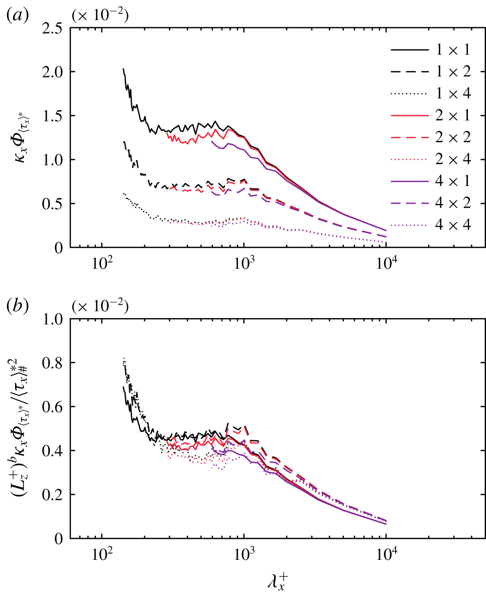
Pre-multiplied streamwise spectra of the universal streamwise wall shear stress averaged over various cell sizes for case RH400-20-4. All spectra in (b) are scaled by  $(L_{z}^{+})^{b}/\langle \unicode[STIX]{x1D70F}_{x}\rangle _{\#}^{\ast 2}$.

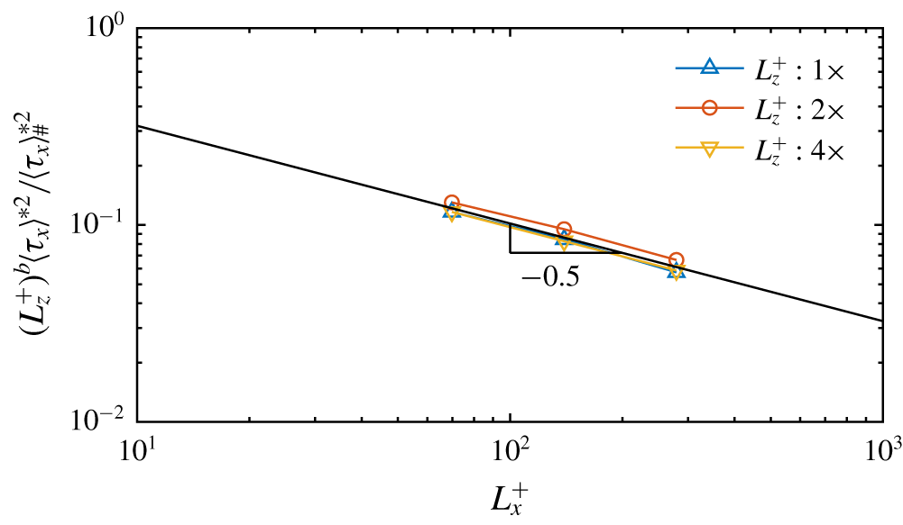
Stress variance scaled by  $\langle \unicode[STIX]{x1D70F}_{x}\rangle _{\#}^{\ast 2}$ and
 $(L_{z}^{+})^{b}$ for RH400-20-4. The straight line represents (4.6) with a slope of
 $-0.5$.

Up to this point, the wall shear stress statistics were averaged only over the minimal cell ‘ $1\times 1$’. However, from the practical point of view of subgrid-scale modelling for LES, it is desirable to investigate these statistics when the averaging cell is larger, typical of those volumes used in an actual ‘wall-modelled’ LES near the wall. The pre-multiplied streamwise spectra of
 $\langle \unicode[STIX]{x1D70F}_{x}\rangle ^{\ast }$ averaged over various cell dimensions for the rough-wall case RH400-20-4 are shown in figure 13(a) as a function of the streamwise wavelength
 $\unicode[STIX]{x1D706}_{x}^{+}$. It is observed that the pre-multiplied spectra collapse relatively well for different cell lengths
 $L_{x}^{+}$ with the same cell width
 $L_{z}^{+}$. However, the stress variance
 $\langle \unicode[STIX]{x1D70F}_{x}\rangle ^{\ast 2}$, which is equal to the area under each spectrum, i.e.
 $$\begin{eqnarray}\langle \unicode[STIX]{x1D70F}_{x}\rangle ^{\ast 2}=\int \unicode[STIX]{x1D705}_{x}\unicode[STIX]{x1D6F7}_{\langle \unicode[STIX]{x1D70F}_{x}\rangle ^{\ast }}\,\text{d}(\text{ln}\unicode[STIX]{x1D705}_{x}),\end{eqnarray}$$
decreases as  $L_{z}^{+}$ increases, suggesting that a power-law dependence is present. Given this observation, a quantitative relation between the stress variance and the dimensions of the spatial averaging cell may be postulated, of the form
 $$\begin{eqnarray}\langle \unicode[STIX]{x1D70F}_{x}\rangle ^{\ast 2}=\langle \unicode[STIX]{x1D70F}_{x}\rangle _{\#}^{\ast 2}(L_{x}^{+})^{-a}(L_{z}^{+})^{-b}.\end{eqnarray}$$
This relationship can be verified by least-squares fitting these data. Figure 14 shows the stress variance  $\langle \unicode[STIX]{x1D70F}_{x}\rangle ^{\ast 2}$ scaled by
 $(L_{z}^{+})^{b}$ and
 $\langle \unicode[STIX]{x1D70F}_{x}\rangle _{\#}^{\ast 2}$ according to (4.6) with
 $\langle \unicode[STIX]{x1D70F}_{x}\rangle _{\#}^{\ast 2}=106.13$ and
 $b=0.98$, plotted as a function of
 $L_{x}^{+}$. It is seen that the scaled
 $\langle \unicode[STIX]{x1D70F}_{x}\rangle ^{\ast 2}$ for various cell widths fall into a single curve with a (negative) slope of
 $a=-0.5$. Similarly, if the pre-multiplied spectra are scaled by
 $(L_{z}^{+})^{b}$ and
 $\langle \unicode[STIX]{x1D70F}_{x}\rangle _{\#}^{\ast 2}$ as shown in figure 13(b), then all spectra are in good agreement despite some discrepancy with larger cell sizes, owing in part to limited statistical samples.
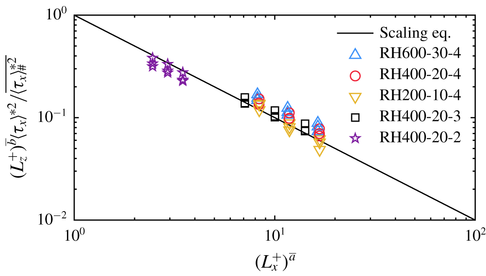
Stress variance  $\langle \unicode[STIX]{x1D70F}_{x}\rangle ^{\ast 2}$ scaled by
 $\overline{\langle \unicode[STIX]{x1D70F}_{x}\rangle _{\#}^{\ast 2}}$ and
 $(L_{z}^{+})^{\bar{b}}$ plotted as a function of
 $(L_{x}^{+})^{\bar{a}}$ for all rough-wall flows, where all parameters are assumed universal for each type of roughness as discussed in the text.

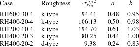
Parameters  $\langle \unicode[STIX]{x1D70F}_{x}\rangle _{\#}^{\ast 2}$,
 $a$ and
 $b$ determined by the least square method for the quantitative relation between the stress variance and cell dimensions based on (4.6).

Table 5 summarizes the parameters  $\langle \unicode[STIX]{x1D70F}_{x}\rangle _{\#}^{\ast 2}$,
 $a$ and
 $b$ for all rough-wall cases, determined by least squares. For all ‘k-type’ roughness,
 $\langle \unicode[STIX]{x1D70F}_{x}\rangle ^{\ast 2}$ shows a consistent power-law dependence on the cell dimensions
 $L_{x}^{+}$ and
 $L_{z}^{+}$, with universal parameters
 $\bar{a}\approx 0.5$ and
 $\bar{b}\approx 1.0$, respectively, denoted by an overbar sign. The constant coefficient
 $\overline{\langle \unicode[STIX]{x1D70F}_{x}\rangle _{\#}^{\ast 2}}\approx 100$ also appears to be universal for all ‘k-type’ roughness. The parameters determined for the case RH200-10-4 deviate from the others possibly due to low-
 $Re$ effects and fewer cell-averaged samples available from DNS. In contrast, for the ‘d-type’ roughness case
 $d/k=2$,
 $\langle \unicode[STIX]{x1D70F}_{x}\rangle ^{\ast 2}$ has a weaker power-law dependence with
 $L_{x}^{+}$ and
 $L_{z}^{+}$, with
 $\bar{a}\approx 0.25$ and
 $\bar{b}\approx 0.8$, while the constant is now
 $\overline{\langle \unicode[STIX]{x1D70F}_{x}\rangle _{\#}^{\ast 2}}\approx 10$.
Figure 15 shows the stress variance  $\langle \unicode[STIX]{x1D70F}_{x}\rangle ^{\ast 2}$ for all cases scaled by
 $(L_{z}^{+})^{\bar{b}}$ and
 $\overline{\langle \unicode[STIX]{x1D70F}_{x}\rangle _{\#}^{\ast 2}}$, plotted as a function of
 $(L_{x}^{+})^{\bar{a}}$, where all parameters are assumed universal for each type of roughness (‘k’ or ‘d’). The straight line demarcates the proposed scaling relation (4.6). In general, the scaled stress variance averaged over various cell dimensions are in good agreement with the proposed relation. The consistency between various roughness cases shown here can be useful in designing candidate wall shear stress models.
5 Conclusions
While the similarity of the outer-layer spatial structure between smooth- and rough-wall flows has been observed by many studies, the detailed descriptions of near-wall turbulence are less well known for flows over rough surfaces. Recently, DNS of turbulent channel flow were performed over hexagonally packed hemispheres at  $Re_{\unicode[STIX]{x1D70F}}=200{-}600$ with inner-scaled roughness height
 $k^{+}=20$ and element spacing
 $d/k=2{-}4$. Flow visualizations of the vortical structures near the rough surface demonstrated the occurrence of coherent packets of hairpin vortices within and outside the roughness sublayer, similar to the observations reported for smooth-wall-bounded flows. In addition, two major vortical structures were identified within the roughness sublayer. First, surface vorticity lines induced by an individual roughness element give rise to a type of vortical structure that persistently covers the frontal surface of each hemisphere. The development of this vortical structure is highly correlated with the surface pressure gradient across the roughness element, which is affected by the separation between elements. Second, a ‘horseshoe’ vortex arises upstream of each hemisphere as a consequence of accumulation of oncoming boundary layer vorticity lines below the stagnation point of each hemisphere, consistent with visualizations of most commonly studied 3-D roughness shapes (for example Castro & Robins Reference Castro and Robins1977; Martinuzzi et al. Reference Martinuzzi, Abuomar and Savory2007). The hexagonal packing of the roughness elements leads to distortion of the trailing vorticity loops of the horseshoe vortices, whose structural attributes downstream depend on roughness packing density.
To understand how these vortical structures contribute to drag, wall shear stress was extracted from DNS by directly integrating the stress tensor over the rough surfaces and then projected along the streamwise direction. Comparison of the roughness function  $\unicode[STIX]{x0394}U^{+}$ as well as the normalized zero-plane displacement
 $d_{0}/k$ between the current hemispherical roughness and other 3-D sharp-edged roughness geometries were made for various element packing densities. It was shown that there is a transition from the ‘k-type’ to ‘d-type’ roughness behaviour and overall reduced drag as the plan area density increased, in accordance with previous work by Placidi & Ganapathisubramani (Reference Placidi and Ganapathisubramani2015). Spectral analysis, particularly on the hemispherical dome, was employed via spherical harmonics to demonstrate the dominant spectral modes associated with the observed vortical structures. It is shown that the inner-scaled power spectra of the streamwise-projected pressure for all rough-wall cases are governed by lower wavemodes that decay fast as the wavemode increases, relatively insensitive to the
 $Re$ effect with fixed
 $k^{+}$, at least for the low to moderate
 $Re$ studied herein. While the power spectra scale well with
 $Re$ for cases with the same element spacing, the energy of spherical harmonic modes decreases significantly as the element spacing decreases. A similar
 $Re$ trend is observed for the spectra of the viscous component, but the dominant mode is the second spherical harmonic mode. The energy of the first and third modes, corresponding to the surface vortical structure and horseshoe vortex, respectively, also decreases substantially with increasing packing density, consistent with the flow visualizations. While this analysis neglects the shear stress generated on the flat horizontal surface, a ‘roughness cell average’ was introduced to quantify the difference of the ignored stress contribution. The minimal unit cells, the dimensions of which depend on the roughness geometry, were used first to yield baseline statistics. Comparison of the minimal roughness-cell-averaged statistics of the viscous contributions shows that the ignored viscous drag is small on the flat section, which becomes less significant when roughness elements are packed more closely. Overall, drag is defined by the pressure contribution, especially at higher
 $Re$, as noted by early work (Raupach et al. Reference Raupach, Antonia and Rajagopalan1991; Jiménez Reference Jiménez2004; Flack & Schultz Reference Flack and Schultz2010).
The paradigm of AM between large-scale structures residing in the outer layer and the wall shear stress was recently identified in high- $Re$ smooth-wall TBLs by Mathis et al. (Reference Mathis, Marusic, Chernyshenko and Hutchins2013). Within this framework, two-point AM correlation coefficients between the low-pass-filtered envelope of the small-scale cell-averaged wall shear stress and large-scale streamwise velocity fluctuation extracted outside the roughness sublayer were explored in this study for both smooth- and rough-wall flows. It is observed that, at the same
 $Re$, the AM correlation is enhanced in the rough-wall flow compared to the smooth-wall flow. In addition, the effect of AM tends to be stronger for the ‘k-type’ roughness (i.e. larger element spacing) in comparison with the ‘d-type’ roughness. Although an increasing
 $Re$ trend of the AM correlation is observed for rough-wall cases with the same element spacing, the dependence of
 $Re$ weakens as
 $Re$ increases.
The inner–outer interactions explored from the perspective of AM highlights the importance of large-scale influences from the inertial region of the flow on the wall shear stress. By exploiting the empirical wall shear stress model originally proposed by Mathis et al. (Reference Mathis, Marusic, Chernyshenko and Hutchins2013), the universal wall shear stress averaged within the minimal roughness unit cell was extracted from the rough-wall flows, leading to more pure statistical information about the wall shear stress without strong effects imparted by the outer-layer LSMs. The pre-multiplied spectra of the minimal cell-averaged universal wall shear stress exhibit consistent large-scale similarity among all roughness cases. However, the behaviours of small scales are roughness-dependent, which shows similar behaviours for ‘k-type’ roughness distinct from ‘d-type’ roughness.
The effect of roughness cell dimensions on the statistics of the cell-averaged universal wall shear stress was investigated from the point of view of practical application in LES. The behaviour of stress variance with respect to the roughness cell dimensions suggests a power-law-based scaling relation, which yields universal agreements for both ‘k-type’ and ‘d-type’ roughness. The consistency shown here can be useful in advancing the modelling of turbulent flows over rough surfaces.
Acknowledgements
This work is supported by the Air Force Office of Scientific Research under grant no. FA9550-14-1-0101 (Dr D. Smith, Program Manager). Computing resources were provided by the DoD High Performance Computing Modernization Program at the ARL, AFRL and ERDC. We gratefully thank Professor P. Fischer for his technical support of the numerical solver and simulation optimizations and Professor W. Anderson for sharing a script to calculate the amplitude modulation correlation.
Declaration of interests
The authors report no conflict of interest.