1. INTRODUCTION
Structural enclosures of modern mechanical products, such as ships hulls, airplanes and automotive bodies, and cases of some electronic devices are fairly complex; hence, it is very expensive, if not impossible, to manufacture them from a single piece of material. Designers therefore have to decompose a complex enclosure into parts such as panels and beams, so that each part could be manufactured with a reasonable cost while satisfying the functional requirements of the assembled enclosure.
As the number of parts increases, however, achieving the dimensional integrity of the final assembly becomes more demanding task due to the inherent variations in manufacturing and assembly operations. For the body structures or frames in which parts are typically forged or bent, it is not economical to manufacture every part with tight tolerance to meet the required dimensional integrity of the final products. For this type of assemblies, it is typical that exact locations of joints (such as welds and fasteners) are not specified in the part design. Instead, it is determined during the assembly operations, when parts are located and fully constrained in fixtures. For this in-process dimensional adjustment to work, the mating surfaces to be joined should allow a small amount of relative motion, which is why those mating surfaces are called slip planes.
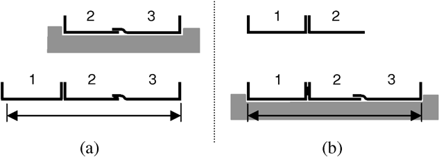
To achieve a desired dimensional integrity of the final assembly, therefore, a designer must determine not only the decomposition of a product but also the orientations of the slip planes, which, in combination, would provide the optimal in-process adjustability of critical dimensions. (See Fig. 1 for two example designs of a rectangular box.) Suppose the distance between section 1 and 3 is critical and parts are assembled on a fixture. Then, it is obvious that the design in Figure 1a is not proper due to its lack of adjustability along the critical dimension. In contrast, the design in Figure 1b provides slip planes such that the relative location of parts can be adjusted along the critical dimension. Although slip planes that are not completely parallel to a critical dimension might allow small motions along the critical dimension, they would yield a motion in other directions as well, which is not desirable.

The design (a) lacks proper slip planes and (b) provides adjustability along the critical dimension.
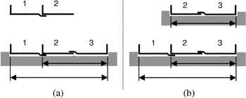
To make things more difficult, the assembly sequences also affect the achievement of critical dimensions as shown in Figure 2 (modified from Whitney et al., 1999). In Figure 2a, parts 2 and 3 are assembled first and then part 1 is put together. However, when part 1 is attached, there is no slip plane parallel to the critical dimension to absorb manufacturing variations that part {2,3} and 1 might carry. In contrast, the sequence shown in Figure 2b provides the slip plane at the assembly step where the critical dimension is achieved, to absorb a variation in length. Figure 3 (modified from Whitney et al., 1999) shows another aspect of interrelation between in-process adjustability and assembly sequence. Although the assembly sequence in Figure 3a realizes both of two critical dimensions at the second assembly step, the sequence in Figure 3b does this one at a time: one critical dimension at the first assembly step, and another one at the second, thereby realizing an independent control of the amount of adjustment in each critical dimension.

Two assembly sequences for an automobile floor plan design, where the total length is critical: (a) poor (cannot adjust total length) and (b) better (can adjust total length).

Two assembly sequences with two overlapping critical dimensions: (a) poor (two critical dimensions adjusted together at an assembly step) and (b) better (each critical dimension independently adjusted at each assembly step).
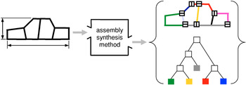
Illustrations from Figures 1, 2, and 3 show that assembly design and assembly sequence are strongly coupled in providing in-process adjustability required for critical dimensions. Provided that the product has a large number of critical dimensions, decomposing the whole product into parts, configuring slip planes, defining datums, assigning tolerances, and planning compatible assembly sequences would be a very tedious task requiring several iterations. This motivated us to develop a systematic method that simultaneously decomposes, selects joints types, and determines an assembly sequence to achieve the optimal in-process adjustability of critical dimensions (Fig. 4).

For a given product geometry, the assembly synthesis method for in-process adjustability suggests desirable decompositions, joint configurations, and assembly sequences (in the form of binary trees). [A color version of this figure can be viewed online at www.journals.cambridge.org]
Assembly synthesis is defined by Yetis and Saitou (2002) as the decomposition of the end product design prior to the detailed component design phase. In our previous work (Lee & Saitou, 2003), we have presented an algorithm of assembly synthesis focused on the in-process adjustability and nonforced fit. The algorithm enumerates all possible assembly syntheses with the accompanying assembly sequences that, in combination, achieve dimensional adjustability for critical dimensions and nonforced fit between parts. It recursively decomposes a product from its final shape into parts and assigns joint configurations according to simple rules drawn from a related literature on assembly design (Whitney et al., 1999). Based on the AND/OR graph for assembly sequence planning (Homem de Mello & Sanderson, 1990), an augmented AND/OR graph has been devised to represent the results.
In the aforementioned work (Lee & Saitou, 2003), slip planes are allowed to take arbitrary angles required for a desired dimensional adjustability. However, in application domains, only a few joint types (such as lap, butt, and lap–butt) or joint angles are available in practice, which may result in slip planes that are not completely parallel to the critical dimensions. As a result, there would be degrees of adjustability (as opposed to simply adjustable or not adjustable) in the results of assembly synthesis, among which the best one should be selected via an optimization process. In addition, the incorporation of the other engineering criteria such as structural stiffness and part manufacturability would increase the computational time, hence rendering an enumeration-based approach impractical without an aid of an optimization process.
As an alternative to an enumeration-based approach (Lee & Saitou, 2003), this paper presents an optimization-based method of assembly synthesis for in-process dimensional adjustability using a genetic algorithm (GA), and its application to a three-dimensional (3-D) automotive space frame. A GA generates candidate assemblies based on a joint library specific for an application domain. Each candidate assembly is evaluated by an internal optimization routine that computes the subassembly partitioning for optimal in-process adjustability, by solving equivalent minimum cut problems on weighted graphs.
2. RELATED WORKS AND BACKGROUNDS
2.1. Assembly model and the key characteristic
An early example of graph-based representation for mechanical assemblies is the “graphe de liaisons fonctionelles” (Bourjault, 1984), where a node and an edge represent each part in an assembly and each physical contact that a pair of parts have between them, respectively. Since then, the representation, typically referred to as the liaison diagram (or liaison graph) after De Fazio and Whitney (1987), has been adopted in many researches in assembly modeling.
The key characteristic (KC) has been defined by Lee and Thornton (1996) as product features, manufacturing process parameters, and assembly features that significantly affect a product's performance, function, and form. To facilitate the realization (or delivery, as often called) of geometric KCs in complex assemblies, Mantripragada and Whitney (1998) devised an augmented liaison diagram called datum flow chain (DFC). The DFC is an efficient tool to analyze how geometric KCs are delivered through datum relationships (represented as directed edges in DFC) among parts and the degrees of freedom joints carry. The critical dimensions mentioned earlier will simply be referred to as KCs in the rest of the paper.
2.2. Assembly sequence generation
Bourjault (1984) and De Fazio and Whitney (1987) are among the earliest researchers in assembly sequence generation. In both works, a user is required to answer a series of questions designed for systematically building the precedence relationships among the liaisons in an assembly, based on which all feasible assembly sequences can be enumerated. Independently, Homem de Mello and Sanderson (1990, 1991a, 1991b) developed an AND/OR graph representation of assembly sequences and presented the first correct and complete algorithm to enumerate all feasible assembly sequences. Under the assumption that an assembly sequence is the reverse of a disassembly sequence, the algorithm generates an AND/OR graph in top-down fashion by recursively partitioning the liaison diagram of an assembly. Since then, numerous research efforts had devoted to extend these pioneering works.
2.3. Design synthesis of mechanical assembly
The aforementioned works on assembly sequence generation and their extensions focus on sequencing the assembly operations of a fixed set of physically separate parts, but do not extend to design synthesis of assembly. Although artificial intelligence (AI) techniques have been applied for many of design synthesis problems (see Antonsson & Cagan, 2001; Cagan et al., 2005, for a comprehensive survey), their application to assembly design for dimensional integrity or manufacturability has been rare. The authors' particular interest is use of decomposition approach used for mechanical assembly design. Wang (1997) presented a method for decomposing an unfolded 3-D geometry of a sheet metal product into parts for improved manufacturability. Their method first unfolds a 3-D product geometry by searching spanning trees of the face-adjacency graph, and then decomposes the unfolded product into several parts by enumerating cut-sets on the spanning trees. Saitou and colleagues have developed a method termed decomposition-based assembly synthesis, for decomposing a given geometry of a structural product into parts for minimum reductions in structural strength (Yetis & Saitou, 2002) and stiffness (Lyu & Saitou, 2003), and for maximum component modularity (Cetin & Saitou, 2001), where a graph representing the topology of a product is directly decomposed for respective criteria, using a GA. Also using a GA, Pollack and Funes (1997) presented a method to synthesize Lego structures meeting certain geometrical requirements. Peysakhov and Regli (2003) extended this work by developing an augmented liaison diagram and genetic operators specifically designed for Lego structures.
2.4. Effect of joint configuration on dimensional variation
Recently, a few researchers have pointed out the effect of joint configurations on the dimensional variations of sheet metal assemblies. Noting the flexibility of sheet metal assemblies, Liu and Hu (1998) utilized engineering structural model combined with statistical analysis to simulate the dimensional variations of a simple rectangular box constructed from three basic joint types: lap, butt, and lap–butt joints. They showed that variation characteristics are different depending on the chosen joint type. Ceglarek and Shi (1998) provided an analysis of joint configurations on their ability of absorbing part variations. Mantripragada and Whitney (1999) presented a state transition model of an assembly sequence, where a joint is viewed as a control vector to absorb variations at each state. Then, optimal control problem is formulated to find the best joint to absorb the variation. Although these works analyze the effect of joint configurations on the dimensional variations of an assembly or finds optimal joints for a given decomposition, none discusses the simultaneous design of product decompositions, joint configurations, and assembly sequences, as addressed in Lee and Saitou (2003) and the present paper.
3. CONCEPTS AND ASSUMPTIONS
Because the assembly synthesis deals with objects yet to be decomposed into an assembly of separate parts, a few terms need to be defined to avoid confusion with generic meanings used in other literatures, including our own previous work.
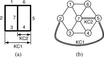
[bull ] A product geometry is a geometric representation of a whole product as one piece (Fig. 5a)
[bull ] A member is a section of a product geometry allowed to be a separate part. A pair of members is connected when they meet at a certain point in the product geometry. It is assumed that, given a product geometry, members are defined by a designer considering manufacturing or functional criteria most suitable to the area of application. Although, in Figure 5a, for example, every segment with constant tangent and no intersection with other segments is defined as a member, a designer might specify sections 1 and 2 as a single member, if he or she wants sections 1 and 2 to be a single part during the assembly synthesis process.
[bull ] A configuration is a group of members that are connected. A product geometry is a configuration, so is a part (as defined below).
[bull ] A configuration graph is a triple:

where M is the set of nodes representing members, T is the set of edges representing connections between a pair of members, and A is the set of edges representing KCs between a pair of members (Fig. 5b). In other words, a configuration graph is a “liaison diagram” of product geometry augmented with the information on KCs. Because a configuration is a group of connected members, a configuration graph excluding the edges in A is a connected graph.1
A graph G is termed connected if every pair of vertices (or nodes) in g are joined by a path (Foulds, 1991).
[bull ] A decomposition is a transition of a configuration into two or more subconfigurations by removing connections between a pair of members.
[bull ] A part is a configuration that cannot be decomposed further under given criteria. An example of such criterion is a minimum part size. Note that a part may consist of one or more members.
[bull ] A joint library is a set of joint types available for a specific application domain. In typical 2-D sheet metal assemblies, lap, butt, and lap–butt joint would form a joint library (Fig. 6).
[bull ] An (synthesized) assembly is a set of parts and joints that connect every part in the set to at least one of other parts in the set. This is what is conventionally referred to as an assembly in the literatures on assembly sequence generation.
[bull ] A liaison graph of a (synthesized) assembly is a triple:

where V0 is the set of nodes representing parts, E0 is the set of edges representing joints, and A0 is the set of edges representing KCs. The A0 takes over all the KCs from the A [Eq. (1)], but connecting the nodes in V0 that are hypernodes of the nodes in M (because a part can consists of one or more nodes). A liaison graph of assembly L0 is often simply referred to as an assembly if obvious from the context.
[bull ] Assembly synthesis is a transformation of a product geometry into an assembly. In other words, a configuration graph C of a product geometry is transformed to a liaison graph of an assembly L0, via assembly synthesis.
[bull ] Subassembly partitioning is (the process of) building a binary tree that represents a (partial) assembly sequence of a synthesized assembly.

A product geometry and its configuration graph.

An example of a joint library for 2-D sheet metal products; LB, a lap–butt joint with lap on the node with lower index and butt on a node with higher index; BL, the opposite configuration.
4. OPTIMAL ASSEMBLY SYNTHESIS FOR IN-PROCESS DIMENSIONAL ADJUSTABILITY
4.1. Overview
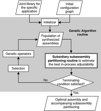
Figure 7 depicts an overview of the proposed method of assembly synthesis for in-process dimensional adjustability. Preliminarily, a designer is supposed to transform a product geometry with KCs to an initial configuration graph, by defining members, and identify joint types available. With the initial configuration graph and the joint library taken as inputs, the method produces an assembly for the product and an accompanying subassembly partitioning that optimally achieve in-process adjustability of the input KCs. The optimization is done with a GA (outer loop) that generates candidate assemblies, and a subsidiary optimizer (nested loop) that estimates the optimal in-process adjustability of the candidate assembly and the accompanying subassembly partitioning. In the following sections, the method will be described in detail with the 2-D skeleton of product geometry shown in Figure 5.

The overview of the proposed method.
4.2. Assembly synthesis with joint library
Using the terminology defined above, the problem of optimal assembly synthesis for in-process adjustability is formulated as follows:

where C is the configuration graph of a (given) product geometry, JL is a (given) joint library, L0 is the liaison graph of the assembly resulting from the joint assignment T [map ] JL onto C, and adjustability is the subsidiary routine (“inner” loop) for subassembly partitioning, which evaluates the dimensional adjustability of L0. Note that the formulation assumes JL includes “connected” to represent no joints. For example, the joint library in Figure 6 is JL = {connected, L, B, LB, BL}. The manufacturability constraints in Eq. (3) depend on the application domain. For example, in the case studies in the last part of this paper, a part carrying KCs is not allowed, because part tolerance is assumed to be much looser than the tolerance required to achieve KCs. A part with a T junction (three members connected to each other) is not allowed, because such shape is not usually manufactured with sheet metals and extruded space frames.
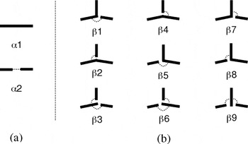
If every joint type can be assigned to every connection, the number of assembly designs to examine is |T ||JL|, which justifies use of heuristic search algorithm such as GA. In the “outer” loop in Figure 7, the GA routine first initializes a population of candidate assemblies (more precisely candidate mappings T [map ] JL). Whereas direct assignment of a joint type from JL to every edge in T could yield a candidate assembly, it might generate physically infeasible or ambiguous joint configurations. Let us consider a connection point (locations where multiple members intersect) such as one where members 1, 6, and 7 meet in Figure 5a. Note that these three members are connected to each other by three edges in its configuration graph (Fig. 5b). If we allow a GA to pick a joint randomly for every edge, it could assign a butt joint between 1 and 6, a lap joint between 1 and 7, and a lap–butt joint between 6 and 7, which is obviously infeasible. In addition, GA might assign “connected” to all three edges, which will result in a T junction. Thus, for connection points with three members, it would be reasonable to assume either a set of a joint between two members and a joint from the other members to one of the two members, or a joint from one member to the other two members connected. For these reasons, in this paper, a GA takes a two-step initialization for each connection point. First, a GA assigns a predefined decomposition type in Figure 8 to a connection point and, second, it assigns joint types (other than “connected”) to broken connections according to selected decomposition type. This method prevents potential infeasible candidate assemblies not only in initialization, but also in simple one-point crossover used in the GA. For each decomposition type in Figure 8, a dotted line represents a joint of a type in a given joint library. Note two-member decompositions have either zero or one joint, whereas three-member decompositions have one or two joint(s).

Decomposition types for (a) two- and (b) three-member connections. A dotted line represents a joint will be assigned between members to which it is attached.
A chromosome, an internal representation of design variables for a GA, is a vector c = (c1, c2,…, cn) of n components, where n is the number of connection points in the product geometry. Each component ci in c is, in turn, a vector of three components:

where di is the decomposition type and ji1 and ji2 are joint types. As specified in Figure 8, di is either α1 or α2 if connection point i is a two-member connection, whereas di can take any value in {β1, β2,…, β9} if connection point i is a three-member connection. Although ji1 and ji2 can take any values specified in the joint library, the value of ji2 is ignored if di indicates the decomposition types with only one joint, and the values of both ji1 and ji2 are ignored if di indicates the decomposition types with only zero joint.
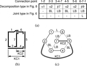
For example, Figure 9a shows a chromosome for the product geometry in Figure 5, where each column represents a component for a connection point denoted by the indices of connecting members. Joint types are chosen from the joint library in Figure 6. Figure 9b and 9c illustrates the assembly represented by the chromosome and the corresponding configuration graphs, respectively. For the evaluation of dimensional adjustability, the configuration graphs in Figure 9c are transformed to a compact liaison graph of the assembly depicted in Figure 10, where each rectangular node represents a part that consists of one or more members.

(a) A chromosome for the product geometry shown in Figure 5, (b) a represented assembly, and (c) corresponding configuration graphs with dotted lines representing joints.

A liaison graph of the assembly in Figure 9c. The members in a configuration are combined into a node, which represents a part in the assembly.
5. OPTIMAL SUBASSEMBLY PARTITIONING
5.1. Binary tree of subassembly partitioning
Each candidate assembly L0 generated by a GA is evaluated for dimensional adjustability by the subsidiary routine (“inner” loop) for subassembly partitioning, represented as the function adjustability in Eq. (3). A subassembly partitioning of a given assembly L0 can be represented as a binary tree (BT),

where S is a set of subsets V of nodes V0 representing parts in subassemblies, and P is a set of hyperedges representing binary partitioning (branching) in the binary tree. Suppose subassembly Li = (Vi, Ei, Ai) is partitioned into two subassemblies Lj = (Vj, Ej, Aj) and Lk = (Vk, Ek, Ak), then the partitioning is represented as a hyperedge p = (Vi, (Vj, Vk)).2
A parenthesized pair of objects usually has an order between the objects. However, in this context, (Vb, Vc) represents a pair of child subassemblies of Va without order. Thus, (Vb, Vc) and (Vc, Vb) are not distinguished in the rest of the paper.

Similarly, we can define a cut-set,3
A cut-set in a connected graph G = (V, E), is a minimal set of edges of E whose removal from G renders G disconnected (Foulds, 1991). In the liason graph we do not count edges representing KC to a cut-set.

Viewing in a reverse (“bottom-up”) fashion, a hyperedge (Vi, (Vj, Vk)) can be interpreted as an assembly process of Vj and Vk into Vi. Under this view, KCp is a set of KCs realized by the assembly operation, and CSp is a set of joints that need to be joined during the assembly of Vj and Vk.
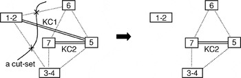
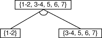
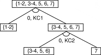
For example, let us consider the liaison graph of assembly L0 = (V0, E0, A0) in Figure 10, where V0 = {1–2, 3–4, 5, 6, 7}, E0 = {(1–2, 3–4), (1–2, 6), (3–4, 7), (3–4, 5), (5, 6), (6, 7)}, and A0 = {(1–2, 5), (5,7)}. If the liaison graph L0 is partitioned into nodes 1–2 and the other nodes as depicted in Figure 11, the corresponding BT has three nodes V0, V1 = {1–2} and V2 = {3–4, 5, 6, 7} in S, and a hyperedge p = [V1, (V2, V3)] in P, of which KCp = {(1–2, 5)} and CSp = {(1–2, 3–4), (1–2, 6)}. A graphical representation of the BT is shown in Figure 12. This binary tree can be interpreted as an assembly sequence consisting on one assembly step: join a subassembly {1–2} with another {3–4, 5, 6, 7} to a final assembly {1–2, 3–4, 5, 6, 7}. Because subassembly {3–4, 5, 6, 7} consists of multiple parts, it is, of course, possible to recursively partition the subassembly into smaller subassemblies, thereby “growing” the binary tree, as discussed later in the section on subassembly partitioning.

A subassembly partitioned into two subassemblies.

A binary tree of the subassembly partitioning illustrated in Figure 11.
5.2. Problem formulation
As observed in Figure 2, it is desirable that a slip plane is provided at the very assembly operation where a KC is realized, and the slip plane is parallel to the KC. In the context of the binary tree of subassembly partitioning, this means at an assembly operation corresponding to a hyperedge p, (the slip planes of) all joints in CSp should be parallel to KCs in KCp.
However, if KCp contains more than one KC in different directions, making all joints in CSp parallel to the KCs is obviously impossible. Therefore, KCp should contain only one KC at every assembly operation corresponding to p. In other words, a partition p should not break more than one KC. This constraint should be kept even if KCs are in the same direction, as achieving more than one KC at a single assembly operation always requires a compromise as illustrated in Figure 3.
Even if KCp contains only one KC, it may not be possible to make all joints in CSp parallel to the KC, depending on the available joint types in the joint library. Therefore, the adjustability of a partition p can be defined as the degree to which joints in CSp are close to the parallel to the KC:

where a is the KC in KCp, e is a joint in CSp, and k(a) and n(e) are the direction vectors of a and e, respectively. Because 0 ≤ |k(aq) · n(e)| ≤ 1, 1 is subtracted from |k(aq) · n(e)| to avoid such cases that the sum of many unparallel joints have the larger value than one parallel joint. As a result, joints of perfect adjustability will yield 0 in Eq. (8), and those of imperfect adjustability will have a negative value measuring their counteradjustability. Although the sum is taken over a ∈ KCp, there should be only one KC in KCp. Based on Eq. (8), the adjustability of a binary tree of subassembly partition BT = (S, P) can be defined as the sum of the adjustabilities of all partitions in P:

The aim of the subsidiary routine adjustability (L0) in Eq. (3) is to find the BT that gives the maximum value of Eq. (9) for a given assembly L0, and return the maximum value to the “outer loop” GA optimizer. Using the aforementioned notations, the problem can be formulated as follows:


Constraints (10a)–(10g) are the definition of BT: constraints (10a)–(10e) are necessary conditions for binary partitioning, and constraint (10f) states the cardinality of KCp is 1, that is, KCp should contain only one KC. Constraint (10g) implies that the BT does not include any nodes or hyperedges that are not successively expanded by the rules (10b) to (10f) from the root node V0.
5.3. Greedy approach for subassembly partitioning
The exact solution to the above optimal subassembly partitioning problem requires a complete AND/OR graph of L0, which, at worst, requires O(3n) decompositions for the assembly with n number of parts (Homem de Mello & Sanderson, 1991b). Because the problem must be solved for each candidate assembly L0 generated by the GA, it is not practical to spend a large amount of time to obtain the true optimal solution. As such, the problem is solved approximately by a greedy approach, where, at each depth of recursion, a subassembly is partitioned into two subassemblies by the cut that provides the maximum adjustability. Starting with the input assembly L0, the recursion proceeds until the resulting subassemblies contain no KCs. In other words, for ∀Vi ∈ S satisfying Ai ≠ Ø in its liaison graph, the partition pi is given as

where Pi is a set of all hyperedges partitioning of Vi satisfying constraints (10b)–(10f) and aq is the only element in KCq [as |KCq| = 1 from (10f)]. Without loss of generality, Eq. (12) can be converted to a minimization:

Because the minimization in Eq. (13) is over all binary partitioning of Li that breaks only one KC, it is equivalent to the minimization over all cut-sets of Li cutting one KC. This is, in turn, equivalent to the minimization over all cut-sets of Li cutting a KC in Ai, followed by the minimization over all KCs in Ai. Namely,

where CS1(a) is a set of cut-sets of Li that do not cut any KCs in Ai other than a. Let min-cut(a) and MCS(a) be the quantity inside of the square brackets in Eq. (14) and its argument, respectively:


As implied by its name, min-cut(a) [and MCS(a) as a result] can be obtained by solving a well-known minimum cut problem on graph (Vi, Ei ∪ Ai[setmn ]{a}) with edge weight

between two nodes incident on a. Because a large weight is assigned to KCs other than a, the solution of the minimum cut problem is the cut-set that only cuts a with the minimum weight, which is MCS(a) in Eq. (16). By solving the minimum cut problem for all a ∈ Ai, one can obtain the optimal cut-set MCS(ai*) of Li, where

and finally pi from MCS(ai*). The following pseudocode outlines the overall algorithm.
greedy-subassembly-partitioning(L0)
1. S ← {V0} and P ← Ø
2. greedy-partitioning(L0, BT)
3. return BT.
greedy-partitioning(Li, BT)
4. If Ai = Ø, return.
5. For each a ∈ Ai, solve the minimum cut problem as defined in Eq. (17) to obtain the min-cut(a).
6. Obtain ai* and the MCS(ai*) from Eq. (18).
7. Obtain partition pi = (Vi, (Vj, Vk)) using MCS(ai*).
8. Partition Li into Lj and Lk using pi.
9. S ← S ∪ {Vj, Vk} and P ← P ∪ {pi}.
10. greedy-partitioning(Lj, BT).
11. greedy-partitioning(Lk, BT).
At termination, greedy-subassembly-partitioning(L0) returns the “fully grown” BT, with which the value of adjustability(L0) in Eq. (3) can be calculated as

Greedy-partitioning is a greedy algorithm that always takes the KCs with the highest adjustability of the current subassembly Li without considering the subsequent partitions. Although the algorithm does not provide the exact solution of the optimal subassembly partitioning problem, it can generate a high-quality solution at moderate computational efforts. It is observed that the problem seems suitable for a greedy strategy because the KC with very low adjustability at the early stages of partitioning (which the algorithm would not pick) tends to become highly adjustable in subsequent stages due to the smaller sizes of subassemblies.
Although greedy-subassembly-partitioning could be used to obtain the optimal assembly sequence for an existing assembly, a dynamic programming algorithm is desired for this purpose because greedy-subassembly- partitioning sacrifices the solution accuracy for speed.
5.4. Optimal subassembly partitioning example
Let us consider again the liaison graph of assembly in Figure 10 and run greedy-subassembly-partitioning with it. Recall L0 = (V0, E0, A0) where V0 = {1–2, 3–4, 5, 6, 7}, E0 = {(1–2, 3–4), (1–2, 6), (3–4, 7), (3–4, 5), (5, 6), (6, 7)}, and A0 = {(1–2, 5), (5,7)}. After initializing S with {V0} and P with an empty set at line 1, a subroutine greedy-partitioning is called at line 2 with L0 and BT:
[bull ] Line 4: greedy-partitioning does not return because A0 is not empty.
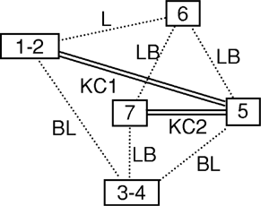
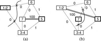
[bull ] Line 5: for two KCs in A0, KC1 = (1–2, 5) and KC2 = (5, 7), the minimum cut problems are formulated based on the geometry in Figure 9b, as illustrated in Figure 13a and b. Note that a large number (100) is assigned to another KC in each figure. Other weights on edges are the same in both figures because the direction vectors of KC1 and KC2 are identical (see Fig. 9b). By inspection, min-cut(KC1) = min-cut(KC2) = 0 as illustrated also in Figure 13a and b.
[bull ] Line 6: Because both KCs have the same value of min-cut, either one can be chosen. Suppose we chose KC1. Then, a0* = KC1 = (1–2, 5) and MCS(a0*) = {(1–2, 6), (1–2, 3–4)} from Figure 13a.
[bull ] Line 7: The corresponding hyperedge is p0 = (V0, (V1, V2)) where V1 = {1–2} and V2 = {3–4, 5, 6, 7}.
[bull ] Line 8: L0 is partitioned into L1 and L2, where V1 = {1–2}, E1 = A1 = Ø, V2 = {3–4, 5, 6, 7}, E2 = {(3–4, 7), (3–4, 5), (5, 6), (6, 7)}, and A2 = {(5,7)}.
[bull ] Line 9: BT is updated with S = {V0, V1, V2} and P = {p0}.
[bull ] Line 10: greedy-partitioning recursively is called with L1 and the updated BT.
[bull ] Line 11: After the return of the recursive call in line 10, greedy-partitioning recursively is called again with L2 and BT (which might have been updates within the recursive call of line 10).

Minimum cuts for (a) KC1 and (b) KC2 for the assembly in Figure 10. In each figure, the respective KC is incident on the nodes with thick lines.
Because A1 is empty, the recursive call of greedy-partitioning at line 10 returns immediately with no update to BT. The recursive call at line 11 proceeds as follows:
[bull ] Line 4: greedy-partitioning does not return because A2 is not empty.
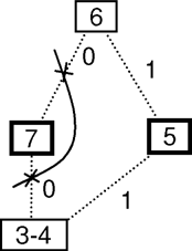
[bull ] Line 5: For KC2 = (5, 7) in A2, the minimum cut problem is formulated as Eq. (16). As illustrated in Figure 14, min-cut(KC2) = 0.
[bull ] Line 6: Because there is only one KC in A2, a2* = KC2 = (5, 7) and MCS(a2*) = {(3–4, 7), (6, 7)} from Figure 14.
[bull ] Line 7: The corresponding hyperedge is p2 = [V2, (V3, V4)], where V3 = {3–4, 5, 6} and V4 = {7}.
[bull ] Line 8: L2 is partitioned into L3 and L4, where V3 = {3–4, 5, 6}, E3 = {(3–4, 5), (5, 6)}, A3 = Ø, V4 = {7}, and E4 = A4 = Ø.
[bull ] Line 9: BT is updated with S = {V0, V1, V2, V3, V4} and P = {p0, p2}.
[bull ] Line 10: greedy-partitioning recursively is called with L3 and the updated BT.
[bull ] Line 11: After the return of the recursive call in line 10, greedy-partitioning recursively is called again with L4 and BT (which might have been updates within the recursive call of line 10).

The minimum cut for KC2 for the subassembly resulting from the partition in Figure 13a.
Because both A3 and A4 are empty, the recursive calls at lines 10 and 11 return immediately with no updates to BT. At this point, the original call of greedy-partitioning(L0, BT) returns, and greedy-subassembly-partitioning(L0) terminates at line 3, by returning the fully grown BT.
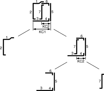
Figure 15 shows a graphical representation of the resulting BT, where the broken KC and its cost at each partitioning are annotated under the corresponding hyperedge. According to the Eq. (19), adjustability(L0) = 0, which means the input assembly L0 with the resulting BT achieves the perfect adjustability of all KCs. This is possible because the orientations of the members (Fig. 9b) and joint types in the library (Fig. 6) can provide the joints exactly parallel to every KC, as illustrated in Figure 16.

Subassembly partitioning for the assembly in Figure 10 by the greedy approach.

Subassembly partitioning in Figure 15 shown in part geometry.
6. 3-D AUTOMOTIVE SPACE FRAME
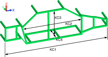
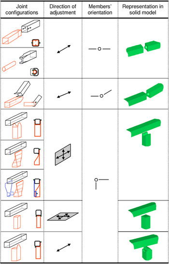
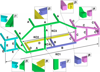
The proposed method is applied to a simplified 3-D model of a real automotive space frame, shown in Figure 17. To reduce the complexity of the problem, four KCs are assumed in this case study. It is also assumed that the frame is made out of extruded aluminum members and every segment with constant tangent and no intersection with other segments is defined as a member. Typical joint types for extruded aluminum members (Malen, 2002) for automotive structures are listed in Figure 18, where the joints with the same dimensional adjustability are regarded as a joint type in the joint library. Depending on the orientations of the mating members, however, not all joint types in Figure 18 are feasible at every connection point in the frame. For example, the butt joint allowed for (nearly) perpendicular connections is not available for coaxial connections. For joints with plane adjustability such as the simple lap joints and butt joints, the normal vector of the plane has been used to compute the inner product with KC in Eq. (17), without subtracting it from 1, such that the cost assigned to those edges is still 0 when the KC is parallel to the plane of adjustability.

A 3-D automotive space frame model with four KCs. In its initial configuration graph, every segment with constant tangent and no intersection with other segments is defined as a member. [A color version of this figure can be viewed online at www.journals.cambridge.org]

A joint library for an automotive space frame (Malen, 2002). Along with the initial configuration graph transformed from the product geometry in Figure 17, it is an input for the GA (see Fig. 7). Adapted with permission. [A color version of this figure can be viewed online at www.journals.cambridge.org]
Because the number of potential joint locations is much larger than the number of KCs in the model, achieving perfect adjustability for all KCs is not very difficult. Therefore, the following two criteria are considered as the objectives to minimize, in addition to the maximization of dimensional adjustability for all KCs:
[bull ] total number of parts: because a smaller number of parts would reduce handling and assembly efforts;
[bull ] sum of the bend angles in all parts: because a straight member with no bends would be the easiest to manufacture with extrusion.
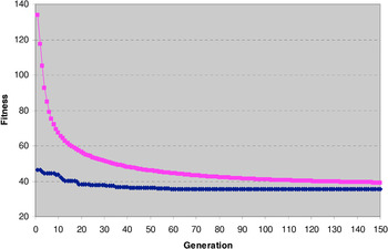
For this particular example, a steady-state GA was used to find solutions, with replacement rate of 0.4 and population size of 1000 over 150 generations. The probability of crossover was 0.8 and that of mutation was 0.2. The GA took 309 s on a 2.0-GHz Pentium 4M PC running Windows. (Refer to Fig. 19 for the GA's behavior.) Considering the huge complexity of enumerative search of assembly design (O(|T ||JL|)) multiplied by the subassembly partitioning (O(3|M|)) for each assembly design, the GA combined with greedy subassembly partitioning shows its efficiency.

Average and minimum fitness values over 150 generations. [A color version of this figure can be viewed online at www.journals.cambridge.org]
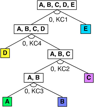
The resulting assembly that achieves perfect adjustability for all four KCs is presented in Figure 20, where joints between subassemblies are magnified. The effects of the additional two criteria on the resulting assembly can be seen by the several long, straight, or nearly straight members, among the shorter members whose joints contribute to the overall adjustability. The accompanying subassembly partitioning is shown in Figure 21, which shows following assembly sequence:
1. Assemble subassembly A with B via joint j7, which provides adjustability required for KC3.
2. Assemble subassembly C and A-B via joint j4 and j8, which provide the adjustability for KC2.
3. Assemble subassembly D and A-B-C via joint j2, j3 and j6, which provide the adjustability for KC4.
4. Assemble subassembly E and A-B-C-D via joint j1 and j5, which provide the adjustability for KC1.

A synthesized assembly from the model in Figure 17 for the optimal in-process adjustability. See Figure 21 for the accompanying subassembly partitioning. [A color version of this figure can be viewed online at www.journals.cambridge.org]

The binary tree of subassembly partitioning for the solution presented in Figure 20. [A color version of this figure can be viewed online at www.journals.cambridge.org]
The computer software used in this example is written in C++ with intense use of data types and algorithms of LEDA developed at Max-Planck-Institut für Informatik, Saarbrücken, Germany. The GA routine is implemented with GALib developed at MIT CADLAB. The C source codes written by Edward Rothberg are used for solving the minimum cut problem, which implement Goldberg and Tarjan's maximum flow algorithm (Goldberg & Tarjan, 1988).
7. SUMMARY AND FUTURE WORKS
This paper presents an optimization-based method of assembly synthesis for in-process dimensional adjustability, where the GA generates candidate assemblies based on a joint library specific for an application domain. Each candidate assembly is evaluated by solving a subassembly partitioning problem for optimal in-process adjustability, posed as an equivalent minimum cut problem on weighted graphs. A case study on a simplified 3-D automotive space frame with four KCs and the accompanying joint library is presented. For real products, the number of KCs depends on the complexity of products and process capabilities. It varies from hundreds for a commercial airplane to only a few for a simple consumer product (see Thornton, 2004; Whitney, 2004, for examples). Those hundreds of KCs are often hierarchical (Thornton, 2004), and for a certain (sub)assembly, the top level KCs are typically in the order of tens or less. When the presented method is applied to those top level KCs for a given (sub)assembly, it decomposes the assembly into its subassemblies until KCs are removed. Then, KCs can be identified for a subassembly partitioned by the method and the method can be reapplied as necessary.
As a future work, the authors plan to extend the approach in Lee and Saitou (2003) to a 3-D model with a joint library, with additional criteria (such as the ones considered in the above example) to prune the enumeration tree of the AND/OR graph of assembly synthesis. For this, major development would be necessary to generalize the concept of nonforced fit introduced in Lee and Saitou (2003) into 3-D assemblies and joints. Currently under development is a unified representation of motion constraints imposed by joints and fixtures tailored for the assembly synthesis process, which will be presented at a future opportunity.
ACKNOWLEDGMENTS
The authors acknowledge Mr. Yasuaki Tsurumi at Toyota Central R&D Laboratory and Prof. Shinji Nishiwaki at Kyoto University for providing us with the body model. We also acknowledge Dr. Malen at the University of Michigan for the joint library of the automotive space frames. This work was supported by a CAREER Award from the National Science Foundation (DMI-9984606). Any opinions, findings, and conclusions or recommendations expressed in this material are those of the authors and do not necessarily reflect the views of the National Science Foundation. A matchable fund for this grant has been provided by Toyota Motor Company. These sources of support are gratefully acknowledged.