2 Self-similar parametrisation of a fracture network

Figure 1.

Schematic of a model network with self-similar variation determined by three parameters: the length factor $\unicode[STIX]{x1D719}^{\ast }$ , the branching factor $\unicode[STIX]{x1D6FC}^{\ast }$ , and the elasticity factor $\unicode[STIX]{x1D702}^{\ast }$ . Each generation, indexed by $i$ , contains $\unicode[STIX]{x1D6FC}^{\ast i}$ identical individual liquid-filled channels, which are modelled as two rigid plates being squeezed together by the elastic medium. The details of the flow near the junctions are not modelled. Although the schematic shows the channels in each generation grouped together, in reality the channels are spread out and have any orientation. In the example shown, $\unicode[STIX]{x1D719}^{\ast }<1$ and $\unicode[STIX]{x1D6FC}^{\ast }=2$ , but any positive real values of $\unicode[STIX]{x1D719}^{\ast }$ , $\unicode[STIX]{x1D6FC}^{\ast }$ and $\unicode[STIX]{x1D702}^{\ast }$ are possible.

We consider a network as a hierarchical structure (see figure 1) originating from a single channel, which we refer to as the outlet or ‘root’ channel with the outlet located at $x^{\ast }=0$ . The outlet is the furthest downstream point and the pressure there (for the study of backflow) is assumed to be zero. Upstream, the root channel splits into a number of identical channels that in turn regularly split upstream in a model geometric progression. The complete set of channels at the same distance (or number of nodes) from the root is referred to as a generation. The network is assumed to have $n$ generations, which we index using $i$ , with $i=0$ signifying the root and $i=n-1$ signifying the ‘tip’ generation, as shown in figure 1. The tip end of the network is the furthest upstream point(s) in the network and flow cannot occur through it. For simplicity, this work does not consider effects resulting from the geometry of the junctions, for example the branching angles. Since we assume that the fluid flows through long fractures separated by short junctions, the effect of the junction geometry will, due to the low Reynolds number, manifest itself mainly as a small change in the overall pressure drop (Dana et al. Reference Dana, Zheng, Peng, Stone, Huppert and Ramon2018). The structure of the network is given using a set of parameters ( $\unicode[STIX]{x1D719}^{\ast },\unicode[STIX]{x1D6FC}^{\ast },\unicode[STIX]{x1D702}^{\ast }$ ) that provide each generation with its own properties related to the previous generation by constant factors.

The branching factor $\unicode[STIX]{x1D6FC}^{\ast }>0$ is the number of branches into which each channel splits, so that the number of channels in the $i$ th generation is ${\unicode[STIX]{x1D6FC}^{\ast }}^{i}$ (where $i$ ranges from 0 to $n-1$ ). Similarly, we assume that the length of each channel in the $i$ th generation is $L{\unicode[STIX]{x1D719}^{\ast }}^{i}$ , where the length factor $\unicode[STIX]{x1D719}^{\ast }>0$ . Finally, the elastic stresses in the medium are assumed to result in a linearly elastic law (see (2.2b ) below) for each channel, with effective elastic modulus (per unit length) $\hat{E}{\unicode[STIX]{x1D702}^{\ast }}^{i}$ in the $i$ th generation, where the elasticity factor $\unicode[STIX]{x1D702}^{\ast }>0$ . For example, for a finite elastic layer, $\hat{E}{\unicode[STIX]{x1D702}^{\ast }}^{i}$ would be its Young’s modulus divided by its original (pre-strained) thickness. The elasticity parameter is such that, when the pressure is uniform, it satisfies $p_{i}^{\ast }={\unicode[STIX]{x1D702}^{\ast }}^{i}\hat{E}h_{i}^{\ast }$ , where $p_{i}^{\ast }$ and $h_{i}^{\ast }$ are the pressure and aperture of the $i$ th fracture. (This set-up is a generalisation of the case $(\unicode[STIX]{x1D719}^{\ast },\unicode[STIX]{x1D6FC}^{\ast },\unicode[STIX]{x1D702}^{\ast })=(1,2,1)$ , i.e. a bifurcating system with uniform elasticity and fracture lengths, studied by Dana et al. (Reference Dana, Zheng, Peng, Stone, Huppert and Ramon2018).)

The simple elasticity law can represent any linearly elastic foundation in which there is no interaction between the different channels. Values for $\unicode[STIX]{x1D702}^{\ast }\neq 1$ represent the medium becoming more ( $\unicode[STIX]{x1D702}^{\ast }>1$ ) or less ( $\unicode[STIX]{x1D702}^{\ast }<1$ ) rigid as the network branches. Various foundations can be emulated by choosing a suitable $\unicode[STIX]{x1D702}^{\ast }$ , including a Winkler foundation (in which case the elastic modulus is the foundation modulus) or a spring array (in which case the elastic modulus is the product of the spring stiffness and the spring density). The factor $\unicode[STIX]{x1D702}^{\ast }$ captures variations in the effective elasticity along the flow path, which include spatial variations in the elasticity of the foundation but also any simple dependence of the elastic behaviour on the channel lengths (in which case $\unicode[STIX]{x1D702}^{\ast }$ would include a dependence on $\unicode[STIX]{x1D719}^{\ast }$ , the length factor) or on the number of channels in the generation due to interaction between them (in which case $\unicode[STIX]{x1D702}^{\ast }$ would include a dependence on $\unicode[STIX]{x1D6FC}^{\ast }$ , the dimensional branching factor). Similarly, the branching factor $\unicode[STIX]{x1D6FC}^{\ast }$ captures the change in the number of channels due to branching, and can also be modified to include the effects of the channel widths (in the third dimension) varying between generations. (This is possible since the model neglects the effects of the junctions on the flow, which results in $\unicode[STIX]{x1D6FC}^{\ast }$ only appearing in the governing equations below as a flux multiplier in (2.3d ).) Hence, although the basic bifurcating set-up in figure 1 implies that $\unicode[STIX]{x1D6FC}^{\ast }$ is an integer and equal to or greater than 2, in fact other positive values of $\unicode[STIX]{x1D6FC}^{\ast }$ are also realistic, and in general we consider any positive values of $\unicode[STIX]{x1D719}^{\ast }$ , $\unicode[STIX]{x1D6FC}^{\ast }$ and  $\unicode[STIX]{x1D702}^{\ast }$ .

2.1 Governing equations

The problem formulation remains similar to that in Dana et al. (Reference Dana, Zheng, Peng, Stone, Huppert and Ramon2018), adjusted by the appropriate parameters. Hence, we give only a brief description of the model here. We define the position variable $x^{\ast }$ to be the distance from the outlet measured along the flow path (see figure 1), and denote the locations of the junctions by

(2.1a,b ) $$\begin{eqnarray}x_{0}^{\ast }=0,\quad x_{i+1}^{\ast }=x_{i}^{\ast }+L{\unicode[STIX]{x1D719}^{\ast }}^{i}.\end{eqnarray}$$

For simplicity, the parallel plates bounding each channel are considered to be rigid and impermeable and therefore the aperture, $h_{i}^{\ast }(t)$ , is solely a function of time. The governing equations for each fracture are then given by the lubrication equation

(2.2a ) $$\begin{eqnarray}\displaystyle \frac{12\unicode[STIX]{x1D707}}{h_{i}^{\ast }(t^{\ast })^{3}}\frac{\text{d}h_{i}^{\ast }(t^{\ast })}{\text{d}t^{\ast }}=\frac{\unicode[STIX]{x2202}^{2}p_{i}^{\ast }(x^{\ast },t^{\ast })}{\unicode[STIX]{x2202}{x^{\ast }}^{2}}\quad (i=0,1,\ldots ,n-1) & & \displaystyle\end{eqnarray}$$

and the force balance

(2.2b ) $$\begin{eqnarray}\displaystyle \int _{x_{i}^{\ast }}^{x_{i+1}^{\ast }}p_{i}^{\ast }(x^{\ast },t^{\ast })\,\text{d}x^{\ast }=\hat{E}{\unicode[STIX]{x1D702}^{\ast }}^{i}L{\unicode[STIX]{x1D719}^{\ast }}^{i}h_{i}^{\ast }(t^{\ast })\quad (i=0,1,\ldots ,n-1). & & \displaystyle\end{eqnarray}$$

The problem now consists of $2n$ equations with $2n$ unknowns, $h_{i}^{\ast }$ and $p_{i}^{\ast }$ . Since each lubrication equation requires an initial condition and two boundary conditions, we require a total of $n$ initial conditions and $2n$ boundary conditions in order to complete the problem statement. These are given by

(2.3a ) $$\begin{eqnarray}\displaystyle h_{i}^{\ast }(0) & = & \displaystyle \frac{p^{\ast }}{\hat{E}{\unicode[STIX]{x1D702}^{\ast }}^{i}}\quad (i=0,1,\ldots ,n-1),\end{eqnarray}$$

(2.3b ) $$\begin{eqnarray}\displaystyle p_{0}^{\ast }(0,t^{\ast }) & = & \displaystyle 0,\end{eqnarray}$$

(2.3c ) $$\begin{eqnarray}\displaystyle p_{i}^{\ast }(x_{i+1}^{\ast },t^{\ast }) & = & \displaystyle p_{i+1}^{\ast }(x_{i+1}^{\ast },t^{\ast })\quad (i=0,1,\ldots ,n-2),\end{eqnarray}$$

(2.3d ) $$\begin{eqnarray}\displaystyle {\unicode[STIX]{x1D6FC}^{\ast }}^{i}{h_{i}^{\ast }}^{3}\left.\frac{\unicode[STIX]{x2202}p_{i}^{\ast }}{\unicode[STIX]{x2202}x^{\ast }}\right|_{(x_{i+1}^{\ast },t^{\ast })} & = & \displaystyle {\unicode[STIX]{x1D6FC}^{\ast }}^{i+1}h_{i+1}^{\ast 3}\left.\frac{\unicode[STIX]{x2202}p_{i+1}^{\ast }}{\unicode[STIX]{x2202}x^{\ast }}\right|_{(x_{i+1}^{\ast },t^{\ast })}\quad (i=0,1,\ldots ,n-2),\qquad\end{eqnarray}$$

(2.3e ) $$\begin{eqnarray}\displaystyle \left.\frac{\unicode[STIX]{x2202}p_{n-1}^{\ast }}{\unicode[STIX]{x2202}x^{\ast }}\right|_{(x_{n}^{\ast },t^{\ast })} & = & \displaystyle 0.\end{eqnarray}$$

The initial condition (2.3a ) corresponds to a uniform initial pressure $p^{\ast }$ , while (2.3c ) and (2.3d ) represent, respectively, continuity of pressure and fluid flux at each node. Finally, (2.3e ) corresponds to no flux at the tip end.

2.2 Non-dimensionalisation

Defining a stretched local coordinate $x$ by

(2.4) $$\begin{eqnarray}x=(x^{\ast }-x_{i})/(L{\unicode[STIX]{x1D719}^{\ast }}^{i})\quad (0\leqslant x\leqslant 1),\end{eqnarray}$$

we non-dimensionalise the system using

(2.5a-c ) $$\begin{eqnarray}h_{i}=h_{i}^{\ast }\left/\left(\frac{p^{\ast }{\unicode[STIX]{x1D719}^{\ast }}^{i}}{\hat{E}}\right)\right.,\quad p_{i}=p_{i}^{\ast }/p^{\ast }\quad \text{and}\quad t=t^{\ast }\left/\left(\frac{12\unicode[STIX]{x1D707}\hat{E}^{2}L^{2}}{{p^{\ast }}^{3}}\right)\right.,\end{eqnarray}$$

as well as length-compensated elasticity and branching factors,

(2.6a,b ) $$\begin{eqnarray}\unicode[STIX]{x1D702}=\unicode[STIX]{x1D702}^{\ast }\unicode[STIX]{x1D719}^{\ast },\quad \unicode[STIX]{x1D6FC}=\unicode[STIX]{x1D6FC}^{\ast }{\unicode[STIX]{x1D719}^{\ast }}^{2}.\end{eqnarray}$$

The resulting dimensionless equations are then

(2.7a,b ) $$\begin{eqnarray}\frac{1}{h_{i}^{3}(t)}\frac{\text{d}h_{i}(t)}{\text{d}t}=\frac{\unicode[STIX]{x2202}^{2}p_{i}(x,t)}{\unicode[STIX]{x2202}x^{2}},\quad \int _{0}^{1}p_{i}(x,t)\,\text{d}x=\unicode[STIX]{x1D702}^{i}h_{i}(t)\quad (i=0,1,\ldots ,n-1),\end{eqnarray}$$

with dimensionless initial and boundary conditions:

(2.8a ) $$\begin{eqnarray}\displaystyle h_{i}(0) & = & \displaystyle \unicode[STIX]{x1D702}^{-i}\quad (i=0,1,\ldots ,n-1),\end{eqnarray}$$

(2.8b ) $$\begin{eqnarray}\displaystyle p_{0}(0,t) & = & \displaystyle 0,\end{eqnarray}$$

(2.8c ) $$\begin{eqnarray}\displaystyle p_{i}(1,t) & = & \displaystyle p_{i+1}(0,t)\quad (i=0,1,\ldots ,n-2),\end{eqnarray}$$

(2.8d ) $$\begin{eqnarray}\displaystyle \unicode[STIX]{x1D6FC}^{i}h_{i}^{3}\left.\frac{\unicode[STIX]{x2202}p_{i}}{\unicode[STIX]{x2202}x}\right|_{(1,t)} & = & \displaystyle \unicode[STIX]{x1D6FC}^{i+1}h_{i+1}^{3}\left.\frac{\unicode[STIX]{x2202}p_{i+1}}{\unicode[STIX]{x2202}x}\right|_{(0,t)}\quad (i=0,1,\ldots ,n-2),\end{eqnarray}$$

(2.8e ) $$\begin{eqnarray}\displaystyle \left.\frac{\unicode[STIX]{x2202}p_{n-1}}{\unicode[STIX]{x2202}x}\right|_{(1,t)} & = & \displaystyle 0.\end{eqnarray}$$

Henceforth, we will omit specifying the range of $i$ when it is clear from the context.

2.2.1 Non-dimensional structure interpretation

An important property of the non-dimensionalisation (2.4)–(2.6) is that it effectively eliminates the length factor $\unicode[STIX]{x1D719}^{\ast }$ from the governing equations, resulting in governing equations (2.7) and (2.8) that essentially describe a network with $(\unicode[STIX]{x1D719}^{\ast },\unicode[STIX]{x1D6FC}^{\ast },\unicode[STIX]{x1D702}^{\ast })=(1,\unicode[STIX]{x1D6FC},\unicode[STIX]{x1D702})$ . Physically, this shows that, in our model, a network with spatially varying channel lengths ( $\unicode[STIX]{x1D719}^{\ast }\neq 1$ ) is dynamically equivalent to a network with spatially uniform channel lengths ( $\unicode[STIX]{x1D719}^{\ast }=1$ ), albeit with modified branching and elasticity factors.

We illustrate this equivalence for the non-dimensional parameter set $(\unicode[STIX]{x1D6FC},\unicode[STIX]{x1D702})=(2,1/2)$ , which we will study in more detail in § 3. This set corresponds, for example, to a network with spatially uniform channel length, each channel splitting into two, and effective elasticity decreasing by a factor of 2 for each generation, i.e. $(\unicode[STIX]{x1D719}^{\ast },\unicode[STIX]{x1D6FC}^{\ast },\unicode[STIX]{x1D702}^{\ast })=(1,2,1/2)$ . It also corresponds to a network with, for example, $(\unicode[STIX]{x1D719}^{\ast },\unicode[STIX]{x1D6FC}^{\ast },\unicode[STIX]{x1D702}^{\ast })=(1/2,8,1)$ , i.e. with decreasing channel lengths, more extreme branching and uniform elasticity. Another possibility is $(\unicode[STIX]{x1D719}^{\ast },\unicode[STIX]{x1D6FC}^{\ast },\unicode[STIX]{x1D702}^{\ast })=(2,1/2,1/4)$ , where the channel length increases ( $\unicode[STIX]{x1D719}^{\ast }>1$ ) and elasticity decreases ( $\unicode[STIX]{x1D702}^{\ast }<1$ ), and $\unicode[STIX]{x1D6FC}^{\ast }<1$ is due to the channel width decreasing faster than the network branches.

Throughout the paper we choose, without loss of generality, to discuss the system using $\unicode[STIX]{x1D719}^{\ast }=1$ , meaning that all the channels in the system are of the same length, $\unicode[STIX]{x1D6FC}=\unicode[STIX]{x1D6FC}^{\ast }$ and  $\unicode[STIX]{x1D702}=\unicode[STIX]{x1D702}^{\ast }$ .

2.3 Reduction to a system of ordinary differential equations

Since we assume that the apertures, $h_{i}(t)$ , have no spatial dependence, we can transform the current form of the governing equations into a ‘discretised’ system of ordinary differential equations (ODEs). We stress that this discretisation is an exact reduction of the model problem and not an approximation of a continuous system.

The pressure field $p_{i}(x,t)$ is expressed using the time-dependent values at the endpoints of the $i$ th channel ( $0\leqslant x\leqslant 1$ ), defined by

(2.9a,b ) $$\begin{eqnarray}\hat{p}_{i}=p_{i}(0,t)\quad \text{and}\quad \hat{p}_{i+1}=p_{i}(1,t),\end{eqnarray}$$

and the respective time-dependent fluxes by

(2.10a,b ) $$\begin{eqnarray}\hat{q}_{i}=\left.\unicode[STIX]{x1D6FC}^{i}h_{i}^{3}\frac{\unicode[STIX]{x2202}p_{i}}{\unicode[STIX]{x2202}x}\right|_{(0,t)}\quad \text{and}\quad \hat{q}_{i+1}=\left.\unicode[STIX]{x1D6FC}^{i}h_{i}^{3}\frac{\unicode[STIX]{x2202}p_{i}}{\unicode[STIX]{x2202}x}\right|_{(1,t)}.\end{eqnarray}$$

The continuity conditions on pressure (2.8c ) and flux (2.8d ) make these definitions consistent between generations.

Integrating the lubrication equation (2.7) in $x$ subject to (2.9), we find that the pressure fields within each generation are given by

(2.11) $$\begin{eqnarray}p_{i}=\hat{p}_{i}(1-x)+\hat{p}_{i+1}x-\frac{{\dot{h}}_{i}}{h_{i}^{3}}\frac{x(1-x)}{2},\end{eqnarray}$$

where the dot operator signifies the time derivative. Substituting the pressure field (2.11) into the force balance (2.7b ), we obtain

(2.12a ) $$\begin{eqnarray}\frac{\hat{p}_{i}+\hat{p}_{i+1}}{2}-\frac{{\dot{h}}_{i}}{12h_{i}^{3}}=\unicode[STIX]{x1D702}^{i}h_{i},\end{eqnarray}$$

where on the left-hand side the average pressure has been simplified to two terms. The first term, which is the average of the endpoint pressures, is due to the first two, linear, terms in the pressure field (2.11). The second term in (2.12a ) is due to the last, nonlinear, term in the pressure field (2.11), which is the squeezing effect, i.e. the contribution of the relaxing elastic matrix to the pressure due to the squeezing of the fluid. Substituting (2.11) into (2.10), we derive the full discretised system of ODEs

(2.12b ) $$\begin{eqnarray}\displaystyle \hat{q}_{i+1}-\hat{q}_{i} & = & \displaystyle \unicode[STIX]{x1D6FC}^{i}{\dot{h}}_{i},\end{eqnarray}$$

(2.12c ) $$\begin{eqnarray}\displaystyle \frac{\hat{q}_{i+1}+\hat{q}_{i}}{2} & = & \displaystyle \unicode[STIX]{x1D6FC}^{i}h_{i}^{3}(\hat{p}_{i+1}-\hat{p}_{i}),\end{eqnarray}$$

with initial and boundary conditions

(2.13a-c ) $$\begin{eqnarray}h_{i}(0)=\unicode[STIX]{x1D702}^{-i},\quad \hat{p}_{0}=0\quad \text{and}\quad \hat{q}_{n}=0.\end{eqnarray}$$

Equation (2.12b ) states that the rate of change of the local volume, $\unicode[STIX]{x1D6FC}^{i}h_{i}$ , in the $i$ th generation and the difference between the inward and outward fluxes must balance and that the local outlet flux is the rate of change of the total upstream volume,

(2.14) $$\begin{eqnarray}\hat{q}_{i}=-\mathop{\sum }_{j=i}^{n-1}\unicode[STIX]{x1D6FC}^{j}{\dot{h}}_{j}.\end{eqnarray}$$

Equation (2.12c ) states that the average flux through each channel is proportional to the pressure drop across it.

The system (2.12) is composed of $n$ time-dependent unknowns $h_{i}$ ( $0\leqslant i\leqslant n-1$ ), $2n+2$ time-dependent unknowns $\hat{p}_{i},\hat{q}_{i}$ ( $0\leqslant i\leqslant n$ ) and $3n$ equations together with two boundary conditions, (2.13b,c ). Since there are time derivatives only for $h_{i}$ , only $n$ initial conditions are needed. The system can be evolved numerically by solving a tridiagonal matrix equation at every time step (see § A.1). The numerical results are obtained using MATLAB’s subroutine ‘ODE23s’.

2.4 Late-time power-law behaviour

Dana et al. (Reference Dana, Zheng, Peng, Stone, Huppert and Ramon2018) showed that, for a network with uniform properties, the late-time dependence of all the network segments is $t^{-1/3}$ . We state that the same late-time scaling applies here and therefore we eliminate time dependence from our equations in order to study the late-time asymptotic behaviour. New similarity variables, $P_{i}(X)$ and $H_{i}$ , are defined by

(2.15a,b ) $$\begin{eqnarray}p_{i}(x,t)=t^{-1/3}P_{i}(X),\quad h_{i}(t)=t^{-1/3}H_{i},\end{eqnarray}$$

and a set of discrete similarity variables, $\hat{P}_{i}$ and $\hat{Q}_{i}$ , by

(2.15c,d ) $$\begin{eqnarray}\hat{p}_{i}(t)=t^{-1/3}\hat{P}_{i},\quad \hat{q}_{i}(t)=t^{-4/3}\hat{Q}_{i},\end{eqnarray}$$

where the hat indicates the value of the continuous function of the $i$ th generation at the point $x=0$ ( $H_{i}$ does not depend on $x$ even though it is not decorated with a hat).

The resulting similarity form of the governing equations (2.12) is then

(2.16a ) $$\begin{eqnarray}\displaystyle \hat{Q}_{i+1}-\hat{Q}_{i} & = & \displaystyle -\unicode[STIX]{x1D6FC}^{i}\frac{H_{i}}{3},\end{eqnarray}$$

(2.16b ) $$\begin{eqnarray}\displaystyle \frac{\hat{Q}_{i+1}+\hat{Q}_{i}}{2} & = & \displaystyle \unicode[STIX]{x1D6FC}^{i}H_{i}^{3}(\hat{P}_{i+1}-\hat{P}_{i}),\end{eqnarray}$$

(2.16c ) $$\begin{eqnarray}\displaystyle \frac{\hat{P}_{i}+\hat{P}_{i+1}}{2}+\frac{1}{36H_{i}^{2}} & = & \displaystyle \unicode[STIX]{x1D702}^{i}H_{i},\end{eqnarray}$$

with boundary conditions

(2.17a,b ) $$\begin{eqnarray}\hat{P}_{0}=0,\quad \hat{Q}_{n}=0.\end{eqnarray}$$

The total fluid volume in each generation $i$ is defined by

(2.18) $$\begin{eqnarray}V_{i}=\unicode[STIX]{x1D6FC}^{i}H_{i},\end{eqnarray}$$

and the outlet flux from the $i$ th channel, $\hat{Q}_{i}$ , can be related to the sum of the upstream volumes by

(2.19) $$\begin{eqnarray}\hat{Q}_{i}=\frac{1}{3}\mathop{\sum }_{j=i}^{n-1}V_{j},\end{eqnarray}$$

where the factor $-1/3$ compared with (2.14) comes from differentiating the total upstream volume of the system with respect to time. Similarly, we can relate the pressure in the downstream point (outlet) of the $i$ th channel to the sum of the downstream pressure drops,

(2.20) $$\begin{eqnarray}\hat{P}_{i}=\mathop{\sum }_{j=0}^{i-1}\unicode[STIX]{x0394}P_{j},\end{eqnarray}$$

where the pressure drop is defined by $\unicode[STIX]{x0394}P_{i}=\hat{P}_{i+1}-\hat{P}_{i}$ .

3 Numerical results

Figure 2.

Numerical solutions for $n=6$ with $\unicode[STIX]{x1D6FC}=2$ and $\unicode[STIX]{x1D702}=1/2$ (i.e. a bifurcating system with decreasing elasticity). (a) Time evolution of the fracture apertures, $h_{i}(t)$ , in both physical non-dimensional space (dashed lines) and multiplied by $t^{1/3}$ so that the results (solid lines) tend to the constants $H_{i}$ according to (2.15b ). (b) Late-time distributions of pressure (solid line), flux (dotted line) and volume (dashed line, equation (2.18)) in the continuous variable $X=x+i$ . The time-scaled distributions along the network are normalised by the maximum calculated values.

In this section, we investigate an example system by solving (2.12) and (2.13) in order to introduce the general method of analysis (see § A.1 for the computational details). We choose the values $\unicode[STIX]{x1D702}=1/2$ and $\unicode[STIX]{x1D6FC}=2$ and note that this case is qualitatively similar to the one presented by Dana et al. (Reference Dana, Zheng, Peng, Stone, Huppert and Ramon2018), where instead $\unicode[STIX]{x1D702}=1$ . As previously mentioned in § 2.2.1, we discuss this example using $\unicode[STIX]{x1D719}^{\ast }=1$ , meaning $\unicode[STIX]{x1D6FC}^{\ast }=2$ and $\unicode[STIX]{x1D702}^{\ast }=1/2$ . The resulting system is a bifurcating network with a decreasing elastic modulus towards the upstream direction (i.e. a ‘soft tip’ system).

The time evolution of the apertures for the case $n=6$ is presented in figure 2(a). At early times, the solution is significantly influenced by the initial condition (2.8a ), while at late times the solution (dashed lines) tends to a $t^{-1/3}$ power law. When multiplied by $t^{1/3}$ , we see that the solution tends to the constants $H_{i}$ (solid lines) according to (2.15b ). The root channel has the smallest aperture, which, according to the elastic equation (2.7b ), is a direct result of the pressure being the smallest at the root together with the root channel having the largest elastic modulus. Furthermore, it is evident that the transition to the late-time behaviour essentially occurs simultaneously in all generations.

The late-time pressure, volume and flux distributions in the network for $n=6$ are presented in figure 2(b). The chosen parameter values yield a somewhat extreme limit, where the pressure gradient is almost entirely concentrated in the root channel and the volume contained in the tip generation is much larger than the downstream volumes. The bifurcation ( $\unicode[STIX]{x1D6FC}>1$ ) causes the majority of the network’s volume to be localised near the tip. This is enhanced by the fact that the softer tip ( $\unicode[STIX]{x1D702}<1$ ) allows the upstream channels to hold more fluid than the downstream ones. Since the volume changes generate the flux (2.19) and the volume is mostly localised at the tip, the flux throughout the rest of the network is approximately constant as shown by the dotted line in figure 2(b). The pressure is approximately constant through much of the network since the pressure drop is concentrated in the root channel.

4 Late-time asymptotic regimes

Figure 3.

Late-time numerical results (thick lines) of pressure and volume distributions for $n=10$ and $(\unicode[STIX]{x1D6FC},\unicode[STIX]{x1D702})$ chosen to yield $\unicode[STIX]{x1D700}_{v}=\unicode[STIX]{x1D700}_{p}=\unicode[STIX]{x1D700}=0.1$ (see § 4). The results are normalised by their maximum values $\hat{p}_{n}$ and $V_{max}$ . Results are for: (a)  $\unicode[STIX]{x1D6FC}=\unicode[STIX]{x1D700}^{1/2}$ , $\unicode[STIX]{x1D702}=\unicode[STIX]{x1D700}^{-3/2}$ , $\hat{p}_{n}=7.23\times 10^{8}$ , $V_{max}=0.51$ ; (b)  $\unicode[STIX]{x1D6FC}=\unicode[STIX]{x1D700}^{-2}$ , $\unicode[STIX]{x1D702}=\unicode[STIX]{x1D700}^{-2}$ , $\hat{p}_{n}=7.25\times 10^{11}$ , $V_{max}=5.13\times 10^{11}$ ; (c)  $\unicode[STIX]{x1D6FC}=\unicode[STIX]{x1D700}^{3/2}$ , $\unicode[STIX]{x1D702}=\unicode[STIX]{x1D700}^{1/2}$ , $\hat{p}_{n}=0.87$ , $V_{max}=0.52$ ; and (d)  $\unicode[STIX]{x1D6FC}=\unicode[STIX]{x1D700}^{-1},\unicode[STIX]{x1D702}=1$ , $\hat{p}_{n}=1.46\times 10^{3}$ , $V_{max}=1.46\times 10^{12}$ . The thinner lines are the asymptotic predictions from § 4, also scaled by the maximum calculated numerical values.

Figure 4.

Numerical results of pressure and volume distributions for $n=10$ and $\unicode[STIX]{x1D700}_{v}=\unicode[STIX]{x1D700}_{p}=\unicode[STIX]{x1D700}=1/2$ (see § 4). The results are normalised by their maximum values $\hat{p}_{n}$ and $V_{max}$ . Results are for: (a)  $\unicode[STIX]{x1D6FC}=\unicode[STIX]{x1D700}^{1/2}$ , $\unicode[STIX]{x1D702}=\unicode[STIX]{x1D700}^{-3/2}$ , $\hat{p}_{n}=4.23\times 10^{2}$ , $V_{max}=6.93\times 10^{-1}$ ; (b)  $\unicode[STIX]{x1D6FC}=\unicode[STIX]{x1D700}^{-2}$ , $\unicode[STIX]{x1D702}=\unicode[STIX]{x1D700}^{-2}$ , $\hat{p}_{n}=3.46\times 10^{3}$ , $V_{max}=3.06\times 10^{3}$ ; (c)  $\unicode[STIX]{x1D6FC}=\unicode[STIX]{x1D700}^{3/2}$ , $\unicode[STIX]{x1D702}=\unicode[STIX]{x1D700}^{1/2}$ , $\hat{p}_{n}=1.65$ , $V_{max}=7.65\times 10^{-1}$ ; and (d)  $\unicode[STIX]{x1D6FC}=\unicode[STIX]{x1D700}^{-1},\unicode[STIX]{x1D702}=1$ , $\hat{p}_{n}=1.6\times 10^{1}$ , $V_{max}=8.17\times 10^{3}$ . The thinner curves show the self-similar interior solution (A 6), from § A.2.2, in (a); a numerical solution for a network of half the size ( $n=5$ ), as discussed in § A.2.3, in (b,c); and the asymptotic result (4.9), derived in § A.2.1, in (d).

In § 3.1, four main asymptotic cases were introduced, dependent on whether the dominant volume (whose change generates the flux) and pressure drop are located at the root ( $i=0$ ) or at the tip ( $i=n-1$ ), as illustrated in figure 3. In this section, we present asymptotic solutions for the four cases and some of their extensions. Examining the behaviour in the various limits allows a better understanding of the system. In each case, we will identify two parameters, ( $\unicode[STIX]{x1D700}_{v},\unicode[STIX]{x1D716}_{p}$ ), depending on $(\unicode[STIX]{x1D6FC},\unicode[STIX]{x1D702})$ , that must be smaller than unity in order for the volume and pressure drop, respectively, to be located at the appropriate end.

4.1 Volume at the tip

4.1.1 Volume at the tip and pressure drop at the root (‘ $V$ : tip, $\unicode[STIX]{x0394}P$ : root’)

We first analyse the case where the volume is localised at the tip and the pressure drop at the root, which includes the examples plotted in figures 2 and 3(d). Based on the observed profiles of the similarity forms $P$ and $V$ along the network, we assume that the pressure is uniform across all the channels except the root ( $P_{i}\approx P$ , for $i\geqslant 1$ ) and that almost all of the volume in the system is contained in the tip channel (i.e. $V\approx V_{n-1}$ ), so that the flux $Q$ is constant along the network except in the tip channel (i.e. $Q_{i}\approx Q$ , for $i\leqslant n-2$ ). When solving the governing equations (2.16a,b ) for $H_{n-1}$ subject to the boundary condition (2.17b ), we find that

(4.1) $$\begin{eqnarray}H_{n-1}^{-2}\sim \hat{P}_{n}-\hat{P}_{n-1}\ll P,\end{eqnarray}$$

since we assume the pressure at both nodes of the tip channel can be approximated as $P$ . We note that, since the pressure is approximately uniform in space, the pressure distribution in a single channel is approximately linear, and the nonlinear term in the force balance (2.16c ) can be neglected. This approximation means that, when the pressure changes little across a channel, then the squeezing effect can be neglected. Then, solving (2.16c ) with (4.1) for $H_{n-1}$ we obtain

(4.2) $$\begin{eqnarray}H_{n-1}=\frac{1}{\unicode[STIX]{x1D702}^{n-1}}P.\end{eqnarray}$$

From (2.19), the flux may now be expressed as

(4.3) $$\begin{eqnarray}Q\approx \frac{1}{3}V_{n-1}=\frac{1}{3}\left(\frac{\unicode[STIX]{x1D6FC}}{\unicode[STIX]{x1D702}}\right)^{n-1}P.\end{eqnarray}$$

Subject to the assumptions that $P_{1}\approx P$ and $Q_{0}\approx Q_{1}\approx Q$ , the governing equations, (2.16b,c ), for the root channel become

(4.4a,b ) $$\begin{eqnarray}Q=H_{0}^{3}P,\quad \frac{P}{2}=H_{0},\end{eqnarray}$$

which yield

(4.5a,b ) $$\begin{eqnarray}H_{0}=(Q/2)^{1/4},\quad P=(8Q)^{1/4}.\end{eqnarray}$$

Combining with the flux expression (4.3), we obtain

(4.6a,b ) $$\begin{eqnarray}P=\frac{2}{3^{1/3}}\left(\frac{\unicode[STIX]{x1D6FC}}{\unicode[STIX]{x1D702}}\right)^{(n-1)/3},\quad Q=\frac{2}{3^{4/3}}\left(\frac{\unicode[STIX]{x1D6FC}}{\unicode[STIX]{x1D702}}\right)^{(4/3)(n-1)}.\end{eqnarray}$$

The leading-order (i.e. assuming uniform pressure) apertures and pressure profiles are thus

(4.7a,b ) $$\begin{eqnarray}H_{0}=P/2,\quad P_{0}(x)=Px,\end{eqnarray}$$

(4.7c,d ) $$\begin{eqnarray}H_{i}=P/\unicode[STIX]{x1D702}^{i},\quad P_{i}(x)=P,\quad \text{for }i\geqslant 1,\end{eqnarray}$$

which are plotted using thinner curves in figure 3(d).

We now calculate an asymptotic error estimate for the localisation of the different features. By considering the volume and pressure drop to be contained in the tip and root, respectively, we have neglected all other pressure drops and volumes in the network. Expressing the volume in each generation as $V_{i}\sim (\unicode[STIX]{x1D6FC}/\unicode[STIX]{x1D702})^{i}P$ , we can estimate the relative error due to neglecting the volume in generation $i=n-2$ (and below) as $\unicode[STIX]{x1D700}_{v}\sim V_{n-2}/V_{n-1}\sim \unicode[STIX]{x1D702}/\unicode[STIX]{x1D6FC}$ . Similarly, for the pressure drop, generally expressed by $\unicode[STIX]{x0394}\hat{P}_{i}\sim Q/(\unicode[STIX]{x1D6FC}^{i}H_{i}^{3})$ , we obtain near the root that $\unicode[STIX]{x1D700}_{p}\sim \unicode[STIX]{x0394}P_{1}/\unicode[STIX]{x0394}P_{0}\sim \unicode[STIX]{x1D702}^{3}/\unicode[STIX]{x1D6FC}$ . The result (4.6) can thus be expected to hold when

(4.8a,b ) $$\begin{eqnarray}\unicode[STIX]{x1D700}_{v}=\frac{\unicode[STIX]{x1D702}}{\unicode[STIX]{x1D6FC}}\ll 1,\quad \unicode[STIX]{x1D700}_{p}=\frac{\unicode[STIX]{x1D702}^{3}}{\unicode[STIX]{x1D6FC}}\ll 1.\end{eqnarray}$$

When exploring other cases we will obtain analogous, but different, expressions for the errors ( $\unicode[STIX]{x1D700}_{v},\unicode[STIX]{x1D700}_{p}$ ) in each regime.

The change in volume or pressure distribution with the respective error estimates $\unicode[STIX]{x1D700}_{v}$ or $\unicode[STIX]{x1D700}_{p}$ is presented in figure 5 for $n=5$ . As can be seen from (4.8), each pair of values $(\unicode[STIX]{x1D700}_{v},\unicode[STIX]{x1D700}_{p})$ corresponds to one set of parameter values, i.e. for the present case $(\unicode[STIX]{x1D6FC},\unicode[STIX]{x1D702})=(\unicode[STIX]{x1D700}_{v}^{-3/2}\unicode[STIX]{x1D700}_{p}^{1/2},\unicode[STIX]{x1D700}_{v}^{-1/2}\unicode[STIX]{x1D700}_{p}^{1/2})$ . Figure 5(a) shows the volume distribution as $\unicode[STIX]{x1D700}_{v}$ is increased from 0.1 to 10 while $\unicode[STIX]{x1D700}_{p}=0.1$ is held fixed. We observe that, as $\unicode[STIX]{x1D700}_{v}\rightarrow 1^{-}$ , the volume that was initially contained in the tip is redistributed more evenly along the network. As $\unicode[STIX]{x1D700}_{v}$ becomes greater than unity, the volume shifts further towards the root end of the network, until the fluid volume is nearly completely contained (by an order of magnitude) in the root channel. Similarly, figure 5(b) shows the pressure distribution as $\unicode[STIX]{x1D700}_{p}$ is increased from 0.1 to 10 while $\unicode[STIX]{x1D700}_{v}=0.1$ is held fixed. When $\unicode[STIX]{x1D700}_{p}\ll 1$ , the shape of the pressure profile is of a boundary layer near the root end. As $\unicode[STIX]{x1D700}_{p}\rightarrow 1^{-}$ , the pressure distribution ‘smears’ over the network, and when $\unicode[STIX]{x1D700}_{p}>1$ , the majority of the pressure drop is located near the tip region.

The arrows in figure 5(c,d) show the path taken by the parameter values $(\unicode[STIX]{x1D6FC},\unicode[STIX]{x1D702})$ (in logarithmic parameter space) corresponding to the five calculations in each upper plot, figure 5(a) and 5(b), respectively. Each arrow points in the same direction as the corresponding arrow in the respective upper plot (i.e. the direction in which the error is increased). The solid lines are the boundaries where the errors equal unity, i.e. $\unicode[STIX]{x1D700}_{v}=\unicode[STIX]{x1D700}_{p}=1$ , for each regime and will be discussed more in § 4.3. The transition through the regime boundaries is in agreement with the intuition that, when the criterion in (4.8) is not fulfilled, the localisation of the appropriate feature is at the opposite end.

In § A.2.1, we present a calculation that considers the volume in multiple channels near the tip of the network and the pressure drop across multiple channels near the root of the network, and hence is expected to hold even for moderate values of $\unicode[STIX]{x1D700}_{v}<1$ and $\unicode[STIX]{x1D700}_{p}<1$ . The result is

(4.9a,b ) $$\begin{eqnarray}P\approx \left[\frac{4}{3}\frac{\unicode[STIX]{x1D700}_{v}^{1-n}}{1-\unicode[STIX]{x1D700}_{v}}\left(\frac{2-\unicode[STIX]{x1D700}_{p}}{1-\unicode[STIX]{x1D700}_{p}}\right)\right]^{1/3},\quad Q\approx \left[\frac{4}{81}\left(\frac{\unicode[STIX]{x1D700}_{v}^{1-n}}{1-\unicode[STIX]{x1D700}_{v}}\right)^{4}\left(\frac{2-\unicode[STIX]{x1D700}_{p}}{1-\unicode[STIX]{x1D700}_{p}}\right)\right]^{1/3},\end{eqnarray}$$

which reduces to the simpler result (4.6) in the limit $\unicode[STIX]{x1D700}_{v}\ll 1$ and $\unicode[STIX]{x1D700}_{p}\ll 1$ .

The case $\unicode[STIX]{x1D6FC}=2$ and $\unicode[STIX]{x1D702}=1$ (i.e. $\unicode[STIX]{x1D700}_{v}=\unicode[STIX]{x1D700}_{p}=1/2$ ) was studied by Dana et al. (Reference Dana, Zheng, Peng, Stone, Huppert and Ramon2018), who presented an asymptotic analysis that allows for moderate values of $\unicode[STIX]{x1D700}_{v}$ (analogous to (A 3)) but requires $\unicode[STIX]{x1D700}_{p}\ll 1$ (analogous to (4.5)) to yield $P=c\times 2^{n}$ , where $c=2/3^{1/3}\approx 1.3867$ . They also solved numerically the asymptotic equation for moderate values of $\unicode[STIX]{x1D700}_{p}$ (analogous to (A 4)) to find $c\approx 1.5875$ , which was a much better approximation to their full numerical results. They concluded that the calculation that considers the pressure drop from multiple channels constitutes a noticeable improvement over the simpler calculation, which only considers the pressure drop from the root channel. Our formula (4.9a ) yields the excellent approximation $c\approx 4^{1/3}\approx 1.5874$ , without the need for a separate numerical calculation for each choice of parameters $(\unicode[STIX]{x1D6FC},\unicode[STIX]{x1D702})$ .

4.1.2 Volume and pressure drop at the tip (‘ $V$ : tip, $\unicode[STIX]{x0394}P$ : tip’)

Figure 5.

Changes in the spatial distributions of the volume and pressure drop along the network for $n=5$ with the change in the respective error parameter ( $\unicode[STIX]{x1D700}_{p}$ or $\unicode[STIX]{x1D700}_{v}$ ) in the range $\{10^{-1},10^{-1/2},10^{0},10^{1/2},10^{1}\}$ . The errors are defined using the ‘volume at the tip and pressure drop at the root’ regime, equation (4.8). Results are for (a) fixed $\unicode[STIX]{x1D700}_{p}$ and (b) fixed $\unicode[STIX]{x1D700}_{v}$ . The arrows in each of the bottom plots, (c,d), are the paths of the corresponding parameter values $(\unicode[STIX]{x1D6FC},\unicode[STIX]{x1D702})$ in their respective upper plot, i.e. (a,b). The solid lines are the regime boundaries (i.e. $\unicode[STIX]{x1D700}_{v}=\unicode[STIX]{x1D700}_{p}=1$ ) as explained in § 4.3.

We continue to investigate the case where the volume is localised near the tip, but now assume that the pressure drop also occurs near the tip as well. Since the dominant pressure drop is located at the tip, i.e. $\hat{P}_{n-1}\ll \hat{P}_{n}$ , the governing equations (2.16) for the tip channel $(i=n-1)$ simplify to

(4.10a-c ) $$\begin{eqnarray}\hat{Q}_{n-1}=\frac{1}{3}\unicode[STIX]{x1D6FC}^{n-1}H_{n-1},\quad \frac{\hat{Q}_{n-1}}{2}=\unicode[STIX]{x1D6FC}^{n-1}H_{n-1}^{3}\hat{P}_{n},\quad \frac{\hat{P}_{n}}{2}+\frac{1}{36H_{n-1}^{2}}=\unicode[STIX]{x1D702}^{n-1}H_{n-1},\end{eqnarray}$$

which are of the same form as the equations for a single isolated channel $(n=1)$ . The solution is

(4.11a-c ) $$\begin{eqnarray}H_{n-1}=\frac{1}{3^{2/3}}\unicode[STIX]{x1D702}^{-(1/3)(n-1)},\quad \hat{P}_{n}=\frac{3^{1/3}}{2}\unicode[STIX]{x1D702}^{(2/3)(n-1)},\quad \hat{Q}_{n-1}=\frac{1}{3^{5/3}}\left(\frac{\unicode[STIX]{x1D6FC}^{3}}{\unicode[STIX]{x1D702}}\right)^{(1/3)(n-1)},\end{eqnarray}$$

and the corresponding (continuous) pressure profile is

(4.12) $$\begin{eqnarray}P_{n-1}(x)=\frac{3^{1/3}}{2}\unicode[STIX]{x1D702}^{(2/3)(n-1)}x(2-x).\end{eqnarray}$$

The flux through the rest of the network is uniform at leading order since we assume that essentially all of the volume is contained in the tip channel and we denote this flux by $Q=\hat{Q}_{0}=\cdots =\hat{Q}_{n-1}$ , equation (4.11c ). In order to solve for the remaining channels ( $i\leqslant n-2$ ), we assume that $\hat{P}_{i}\ll \hat{P}_{i+1}$ . The governing equations (2.16) then simplify to

(4.13a,b ) $$\begin{eqnarray}Q=\unicode[STIX]{x1D6FC}^{i}H_{i}^{3}\hat{P}_{i+1},\quad \frac{\hat{P}_{i+1}}{2}=\unicode[STIX]{x1D702}^{i}H_{i},\end{eqnarray}$$

which yield

(4.14a-c ) $$\begin{eqnarray}H_{i}=\left(\frac{1}{\unicode[STIX]{x1D702}\unicode[STIX]{x1D6FC}}\right)^{i/4}\left(\frac{Q}{2}\right)^{1/4},\quad \hat{P}_{i+1}=\frac{Q}{\unicode[STIX]{x1D6FC}^{i}H_{i}^{3}},\quad P_{i}(x)=\frac{Q}{\unicode[STIX]{x1D6FC}^{i}H_{i}^{3}}x.\end{eqnarray}$$

Requiring that $V_{n-2}\ll V_{n-1}$ and $\hat{P}_{n-2}\ll \hat{P}_{n-1}$ , we obtain the error estimates $\unicode[STIX]{x1D700}_{v}$ and $\unicode[STIX]{x1D700}_{p}$ , and the conditions for our assumptions to hold, as

(4.15a,b ) $$\begin{eqnarray}\unicode[STIX]{x1D700}_{v}=\left(\frac{\unicode[STIX]{x1D702}}{\unicode[STIX]{x1D6FC}^{3}}\right)^{1/4}\ll 1,\quad \unicode[STIX]{x1D700}_{p}=\left(\frac{\unicode[STIX]{x1D6FC}}{\unicode[STIX]{x1D702}^{3}}\right)^{1/4}\ll 1.\end{eqnarray}$$

These expressions are different from those derived above in (4.8), but the common boundary between the two regimes is given by $\unicode[STIX]{x1D700}_{p}=1$ , i.e. $\unicode[STIX]{x1D6FC}=\unicode[STIX]{x1D702}^{3}$ , in both cases, as is to be expected. The boundary between the two regimes can also be demonstrated by holding $\unicode[STIX]{x1D700}_{v}=0.1$ fixed and letting $\unicode[STIX]{x1D700}_{p}$ grow beyond unity. This is shown in figure 5(b) starting from the ‘volume at root, pressure drop at tip’ regime. The pressure drop, previously contained at the root, slowly spreads along the network. Once $\unicode[STIX]{x1D700}_{p}>1$ , the pressure drop starts concentrating towards the tip end of the network to achieve the current regime. Figure 5 will be discussed further in § 4.3.

4.2 Volume at the root

When essentially all of the volume is contained in the root channel ( $i=0$ ), there is almost no flux from the remainder of the network (i.e. $\hat{Q}_{1}\ll \hat{Q}_{0}$ ). Hence, the system behaves like an isolated channel, satisfying

(4.16a-c ) $$\begin{eqnarray}\hat{Q}_{0}=\frac{1}{3}H_{0},\quad \frac{\hat{Q}_{0}}{2}=H_{0}^{3}\hat{P}_{1},\quad \frac{\hat{P}_{1}}{2}+\frac{1}{36H_{0}^{2}}=H_{0},\end{eqnarray}$$

which yields

(4.17a-d ) $$\begin{eqnarray}H_{0}=\frac{1}{3^{2/3}},\quad \hat{P}_{1}=\frac{3^{1/3}}{2},\quad P_{0}(x)=\frac{3^{1/3}}{2}x(2-x),\quad \hat{Q}_{0}=\frac{1}{3^{5/3}.}\end{eqnarray}$$

To account for the upstream pressures, we can estimate the $i$ th pressure drop, $\unicode[STIX]{x0394}\hat{P}_{i}$ , using a scaling argument. Since for each generation $i$ , the upstream volume is negligible compared with the local volume (i.e. $V_{i+1}\ll V_{i}$ ), the flux through the $i$ th channel scales as the local volume, $\unicode[STIX]{x1D6FC}^{i}H_{i}^{3}\unicode[STIX]{x0394}\hat{P}_{i}\sim \unicode[STIX]{x1D6FC}^{i}H_{i}$ , which yields

(4.18) $$\begin{eqnarray}\unicode[STIX]{x0394}\hat{P}_{i}\sim H_{i}^{-2}.\end{eqnarray}$$

4.2.1 Volume and pressure drop at the root (‘ $V$ : root, $\unicode[STIX]{x0394}P$ : root’)

When both the volume and the pressure drop are localised near the outlet ( $i=0$ ), the pressure in the remainder of the network is again assumed to be approximately uniform at $P=\hat{P}_{1}=3^{1/3}/2$ (which is thus also the maximum pressure). Hence, the solution is

(4.19a-c ) $$\begin{eqnarray}\hat{Q}_{i}=\unicode[STIX]{x1D6FC}^{i}\frac{H_{i}}{3},\quad \hat{P}_{i}=P_{i}(x)=P,\quad H_{i}=\frac{P}{\unicode[STIX]{x1D702}^{i}},\quad 1\leqslant i\leqslant n-1.\end{eqnarray}$$

The resulting local volumes $V_{i}=(\unicode[STIX]{x1D6FC}/\unicode[STIX]{x1D702})^{i}P$ and the pressure drops $\unicode[STIX]{x0394}\hat{P}_{i}\sim \unicode[STIX]{x1D702}^{2i}P^{-2}$ must decay, so we require

(4.20a,b ) $$\begin{eqnarray}\unicode[STIX]{x1D700}_{v}=\frac{\unicode[STIX]{x1D6FC}}{\unicode[STIX]{x1D702}}\ll 1,\quad \unicode[STIX]{x1D700}_{p}=\unicode[STIX]{x1D702}^{2}\ll 1\end{eqnarray}$$

for our solution to hold.

4.2.2 Volume at the root and pressure drop at the tip (‘ $V$ : root, $\unicode[STIX]{x0394}P$ : tip’)

When the pressure drops increase upstream, the local pressure drop is also an estimate for the local pressure. Similar to (4.18), we obtain the balance

(4.21a,b ) $$\begin{eqnarray}\hat{Q}_{i}=\unicode[STIX]{x1D6FC}^{i}\frac{H_{i}}{3},\quad \hat{P}_{i}\sim \unicode[STIX]{x0394}\hat{P}_{i}\sim H_{i}^{-2}\sim \unicode[STIX]{x1D702}^{i}H_{i},\end{eqnarray}$$

which implies

(4.22a-c ) $$\begin{eqnarray}\hat{Q}_{i}\approx \frac{1}{3}\left(\frac{\unicode[STIX]{x1D6FC}}{\unicode[STIX]{x1D702}^{1/3}}\right)^{i},\quad H_{i}\approx \unicode[STIX]{x1D702}^{-i/3},\quad \hat{P}_{i}\approx \unicode[STIX]{x1D702}^{2i/3}.\end{eqnarray}$$

The conditions for rapidly decaying volume $V_{i}=(\unicode[STIX]{x1D6FC}/\unicode[STIX]{x1D702}^{1/3})^{i}$ and increasing pressure $\hat{P}_{i}$ , (4.22c ), then yield

(4.23a,b ) $$\begin{eqnarray}\unicode[STIX]{x1D700}_{v}=\frac{\unicode[STIX]{x1D6FC}}{\unicode[STIX]{x1D702}^{1/3}}\ll 1,\quad \unicode[STIX]{x1D700}_{p}=\unicode[STIX]{x1D702}^{-2/3}\ll 1.\end{eqnarray}$$

Since the volume decays ( $\hat{Q}_{i+1}\ll \hat{Q}_{i}$ ) and pressure grows rapidly ( $\hat{P}_{i+1}\gg \hat{P}_{i}$ ), each individual section behaves like an isolated channel,

(4.24a-c ) $$\begin{eqnarray}\hat{Q}_{i}=\frac{1}{3}\unicode[STIX]{x1D6FC}^{i}H_{i},\quad \frac{\hat{Q}_{i}}{2}=\unicode[STIX]{x1D6FC}^{i}H_{i}^{3}\hat{P}_{i+1},\quad \frac{\hat{P}_{i+1}}{2}+\frac{1}{36H_{i}^{2}}=\unicode[STIX]{x1D702}^{i}H_{i},\end{eqnarray}$$

which yields

(4.25a-d ) $$\begin{eqnarray}\displaystyle H_{i}=\frac{\unicode[STIX]{x1D702}^{-i/3}}{3^{2/3}},\quad \hat{P}_{i+1}=\frac{3^{1/3}}{2}\unicode[STIX]{x1D702}^{2i/3},\quad P_{i}(x)=\frac{3^{1/3}}{2}\unicode[STIX]{x1D702}^{2i/3}x(2-x),\quad \hat{Q}_{i}=\frac{1}{3^{5/3}}\left(\frac{\unicode[STIX]{x1D6FC}}{\unicode[STIX]{x1D702}^{1/3}}\right)^{i}. & & \displaystyle \nonumber\\ \displaystyle & & \displaystyle\end{eqnarray}$$

The maximum pressure is

(4.26) $$\begin{eqnarray}\hat{P}_{n}=\frac{3^{1/3}}{2}\unicode[STIX]{x1D702}^{(2/3)(n-1)}.\end{eqnarray}$$

4.3 Summary and the regime plot

We have derived the late-time asymptotic solutions for the flux, aperture and pressure distribution along the network for the four cases, i.e. the bulk of the volume and pressure drop is localised near either the root or tip end. In each case the volume and pressure distributions are assumed to be localised at an edge by neglecting all other volumes and pressure drops along the network. For each of the obtained solutions, estimates for the asymptotic error, $\unicode[STIX]{x1D700}_{v}$ and $\unicode[STIX]{x1D700}_{p}$ , have been calculated. We can see that asymptotic results for $n=10$ plotted along with the numerical results in figure 3 show a good agreement to the order of $O(\unicode[STIX]{x1D700}_{v},\unicode[STIX]{x1D700}_{p})$ as expected. This gives us confidence in our derivation and we continue in describing the late-time asymptotic results of the model.

We proceed to look at the error estimates derived in the different regimes. In figure 5(a), we see that, for a fixed $\unicode[STIX]{x1D700}_{p}=0.1$ , relaxing $\unicode[STIX]{x1D700}_{v}$ towards unity results in the spreading of the volume along the network (towards the root). When $\unicode[STIX]{x1D700}_{v}$ becomes much larger than unity, the volume begins collecting near the root channel. The system then approaches the distinct limit where both volume and pressure drop are contained in the root. The arrows in figure 5(c,d) indicate the path of values of the chosen parameter sets in figure 5(a,b) respectively. As seen in figure 5(b), for a fixed $\unicode[STIX]{x1D700}_{v}=0.1$ , relaxing $\unicode[STIX]{x1D700}_{p}$ towards unity results in a spreading of the pressure drop along the network (towards the tip). When $\unicode[STIX]{x1D700}_{p}$ is larger than unity, the pressure drop collects near the tip channel. The system then approaches the distinct limit where both volume and pressure are contained in the tip.

Figure 6.

An asymptotic regime diagram plotted on a logarithmic scale of $(\unicode[STIX]{x1D6FC},\unicode[STIX]{x1D702})$ space. In each region, bounded by the solid lines $\unicode[STIX]{x1D700}_{v}=1$ or $\unicode[STIX]{x1D700}_{p}=1$ , the volume and the pressure drop are localised near either the root ( $i=0$ ) or the tip ( $i=n-1$ ). In the unshaded regions, bounded by the dashed lines, i.e. $\unicode[STIX]{x1D700}_{v}=0.1$ or $\unicode[STIX]{x1D700}_{p}=0.1$ , the volume and pressure drop are approximately localised to a single channel near the root or tip. In the shaded region, one or both are spread out over multiple channels. The round markers are the parameter values for the numerical results presented in figure 3, based on $\unicode[STIX]{x1D700}_{v}=\unicode[STIX]{x1D700}_{p}=0.1$ . The triangle is the parameter set used in figure 2.

We now present a schematic regime diagram (figure 6) in logarithmic $(\unicode[STIX]{x1D6FC},\unicode[STIX]{x1D702})$ space, showing at which end the volume and pressure drop are concentrated for any given set of values. Typically, moving to the right in the diagram (i.e. increasing $\unicode[STIX]{x1D6FC}$ ) increases the number of branches at the tip end of the network, which causes the volume to shift towards the tip. Moving up in the diagram (i.e. increasing $\unicode[STIX]{x1D702}$ ) increases the rigidity near the tip end and hence can be expected to reduce the apertures at the tip end and cause the pressure drop there to increase. The solid lines (corresponding to $\unicode[STIX]{x1D700}_{v}=1$ or $\unicode[STIX]{x1D700}_{p}=1$ for each of the regimes) are the actual regime boundaries, so that crossing them means the transition of the relevant feature (volume or pressure drop) from being mostly contained near the given end (according to the current regime) towards being mostly contained near the opposite end. For example, the parameter set marked with a triangle in figure 6 (presented in figure 2) are in the ‘volume at tip, pressure drop at root’ regime. The further away from the relevant solid line, the smaller the error value. If we move towards the upper solid line (i.e. $\unicode[STIX]{x1D700}_{p}=1$ ) then $\unicode[STIX]{x1D700}_{p}$ grows. Similarly, approaching the solid line located in the bottom left quadrant (i.e. $\unicode[STIX]{x1D700}_{v}=1$ ) means $\unicode[STIX]{x1D700}_{v}$ grows.

The dashed contours in figure 6 show where the asymptotic error of the results derived in this section is 10 %, i.e. $\unicode[STIX]{x1D700}_{v}=0.1$ or $\unicode[STIX]{x1D700}_{p}=0.1$ . Outside these lines, in the unshaded regions, we consider the volume and pressure drop to each be truly localised to a single generation of channels, such as for the cases shown in figure 3, which correspond to the four intersections of the dashed lines (round markers in figure 6). Inside these lines, in the shaded region, as shown in figure 4 for $\unicode[STIX]{x1D700}_{v}=\unicode[STIX]{x1D700}_{p}=1/2$ , the volume and pressure drop remain localised near the root or tip end of the network, but spread out across multiple generations of channels rather than being contained in a single generation. We investigate this region of parameter space in more detail in appendix A, and show that the main physical principles remain the same.

5 Drainage time

Figure 7.

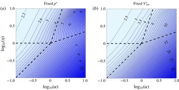
Contour plots of the time $t_{90}^{\ast }$ for a network with $n=5$ to evict 90 % of its initial volume, for two different non-dimensionalisations. (a) The original non-dimensionalisation (2.5c ), based on initial pressure $p^{\ast }$ , $\log _{10}(t_{90})$ . (b) A non-dimensionalisation (5.3) based on initial volume $V_{init}^{\ast }$ , $\log _{10}(\tilde{t}_{90})=\log _{10}(t_{90}V_{init}^{3})$ . The dashed lines are the regime boundaries from figure 6.

In addition to the late-time dynamics and volume and pressure distributions studied in § 4, the early-time dynamics is also of great importance for the hydraulic fracturing industry, in particular with regards to wastewater management and hydrocarbon production planning. The operation of hydraulic fracturing wells necessitates better management and prediction of the backflow quantities, and time scales, of the injected fracturing fluids. It is useful to define a measure for comparison of the behaviour of different network structures, based on the relative amount of volumetric flux they produce in a given time period, i.e. how fast is drainage.

We measure the drainage relative to the initial volume $V_{init}^{\ast }$ (non-dimensionalised to $V_{init}$ ), defined by

(5.1) $$\begin{eqnarray}V_{init}^{\ast }=\mathop{\sum }_{i=0}^{n-1}\left(\frac{\unicode[STIX]{x1D6FC}^{\ast }\unicode[STIX]{x1D719}^{\ast }}{\unicode[STIX]{x1D702}^{\ast }}\right)^{i}\frac{p^{\ast }L}{\hat{E}}=\frac{p^{\ast }L}{\hat{E}}V_{init},\quad \text{i.e. }V_{init}=\mathop{\sum }_{i=0}^{n-1}\left(\frac{\unicode[STIX]{x1D6FC}}{\unicode[STIX]{x1D702}}\right)^{i},\end{eqnarray}$$

and compare drainage efficiency using the time

(5.2) $$\begin{eqnarray}t_{90}^{\ast }=\frac{12\unicode[STIX]{x1D707}\hat{E}^{2}L^{2}}{p^{\ast 3}}t_{90}\end{eqnarray}$$

that it takes for 90 % of the initial volume to be ejected from the system. (The value 90 % is somewhat arbitrary, but should give a good indication of how drainage efficiency varies with $\unicode[STIX]{x1D6FC}$ and $\unicode[STIX]{x1D702}$ in general.)

Calculated values of $\log _{10}(t_{90})$ are presented for different parameter values in figure 7 for $n=5$ . Glancing at the trends presented in figure 7(a), we can immediately see a general decrease in drainage efficiency from the top left quadrant (‘volume at root, pressure drop at tip’) towards the bottom right quadrant (‘volume at tip, pressure drop at root’). This trend is a result of two distinct physical effects. Firstly, an increase in the branching factor $\unicode[STIX]{x1D6FC}$ shifts the initial volume towards the tip end of the network and hence delays the drainage. (Although not shown, for certain scaling forms, this trend is further enhanced with an increase in $n$ as the bulk volume is moved further away from the outlet (Dana et al. Reference Dana, Zheng, Peng, Stone, Huppert and Ramon2018).) Secondly, an increase of the elasticity factor $\unicode[STIX]{x1D702}$ has the reverse effect, shifting the volume towards the root and enhancing the evacuation rate (since the rigid tip is more effective at expelling the fluids). As a consequence, the network is least efficient when $\unicode[STIX]{x1D6FC}\gg 1$ and $\unicode[STIX]{x1D702}\ll 1$ , i.e. in the asymptotic regime with volume at the tip and pressure drop at the root.

Looking more closely at the upper right corner of figure 7(a), we find that the curved contours indicate non-monotonicity in $\unicode[STIX]{x1D702}$ : for example, for $\unicode[STIX]{x1D6FC}=10^{1/2}$ , as $\unicode[STIX]{x1D702}$ increases, $t_{90}$ initially decreases as expected, but then increases for a while, before decreasing again. This is due to the varying initial volume in the network, as we shall now show.

The non-dimensional initial volume $V_{init}$ (5.1) varies with $\unicode[STIX]{x1D6FC}$ (by the addition of more branches) and $\unicode[STIX]{x1D702}$ (by the change of the initial apertures), so figure 7(a) is comparing the evacuation times of networks with different initial volume (but with the same initial pressure). This can yield misleading results even though $t_{90}$ is defined relative to the initial volume. If we consider two physical systems with different $\unicode[STIX]{x1D6FC}^{\ast }$ and $\unicode[STIX]{x1D702}^{\ast }$ but the same initial volume $V_{init}^{\ast }$ , then their different initial pressures $p^{\ast }$ result in the drainage times $t_{90}^{\ast }$ being non-dimensionalised using different time scales (2.5c ). Hence comparing the values of $t_{90}$ can yield the opposite result to comparing the original values $t_{90}^{\ast }$ .

Thus, for a direct comparison, we need to replace the non-dimensionalisation (2.5), which is based on the initial pressure $p^{\ast }$ , with a non-dimensionalisation based on initial volume $V_{init}^{\ast }$ , such as

(5.3a-c ) $$\begin{eqnarray}\tilde{h}_{i}=h_{i}^{\ast }\left/\left(\frac{V_{init}^{\ast }}{L}\right)\right.,\quad \tilde{p}_{i}=p_{i}^{\ast }\left/\left(\frac{\hat{E}V_{init}^{\ast }}{L}\right)\right.\quad \text{and}\quad \tilde{t}=t^{\ast }\left/\left(\frac{12\unicode[STIX]{x1D707}L^{5}}{\hat{E}V_{init}^{\ast 3}}\right)\right.,\end{eqnarray}$$

where the tildes indicate the new rescaling. (The spatial variable $x$ remains the same.) These are related to the original non-dimensional variables (2.5) by

(5.4a-c ) $$\begin{eqnarray}\frac{\tilde{h}_{i}}{h_{i}}=V_{init},\quad \frac{\tilde{p}_{i}}{p_{i}}=V_{init}\quad \text{and}\quad \frac{\tilde{t}}{t}=V_{init}^{3},\end{eqnarray}$$

where $V_{init}$ is the initial volume (5.1) under the original non-dimensionalisation.

The contour plot of drainage time for the new non-dimensionalisation (5.3) is shown in figure 7(b). The result for $\tilde{t}$ is now monotonic in both $\unicode[STIX]{x1D6FC}$ and $\unicode[STIX]{x1D702}$ , which confirms the intuitive explanations presented above. We conclude that the non-monotonicity observed in the upper right corner of figure 7(a) is simply due to the variation of initial volume (5.1) with $\unicode[STIX]{x1D6FC}$ (which adds branches) and $\unicode[STIX]{x1D702}$ (which affects the initial apertures).

We can also conclude that, in general, when comparing non-dimensional results for $t_{90}^{\ast }$ , one must be aware of which parameters were used in the non-dimensionalisation and hence must be considered fixed in order for the comparison to be valid. For example, when comparing the effect of the number of generations $n$ on the drainage efficiency, the results can differ depending on which length is held fixed: the length $L$ of a single channel or the length $L\sum _{i=0}^{n-1}\unicode[STIX]{x1D719}^{\ast i}$ of the entire network. Yet another possibility is that no particular length is fixed, and instead, for example, both the initial volume $V_{init}^{\ast }$ and the initial pressure $p^{\ast }$ are held fixed.

6 Summary and discussion

In this paper we have considered fluid flow out of a relaxing fracture network characterised by parameters accounting for a branching factor and spatially varying length and elastic modulus. This is an extension of the case considered by Dana et al. (Reference Dana, Zheng, Peng, Stone, Huppert and Ramon2018) that assumed these properties to be uniform. The variations were described by a self-similar model, in which each property (channel length, number of channels in a generation or elastic modulus) is multiplied by an additional single factor $\unicode[STIX]{x1D719}^{\ast }$ , $\unicode[STIX]{x1D6FC}^{\ast }$ or $\unicode[STIX]{x1D702}^{\ast }$ with every further generation upstream. We used numerical results (figure 3) for various parameter values that provide distinct volume and pressure distributions along the network, which led to characterising the entire parameter space using four main regimes based on the localisation of the fluid volume and pressure drop. For example, when the pressure drop is localised near the root, the network can be approximated as a reservoir with a uniform pressure along the network, and when the volume is near the tip, the flux can be considered as uniform along the flow path. Conversely, when the pressure drop is near the tip and the volume near the root, each channel behaves like an isolated channel, not feeling the effects of its upstream neighbours.

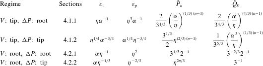
Asymptotic solutions for the time evolution of the apertures, pressure profiles and outlet flux were found for each regime (see summary of results in table 1) in the main cases where the fluid volume and pressure drop are concentrated in a single generation of channels at either end of the network. The predicted values agree well with the numerical results to the order of error suggested for the parameters in each regime, i.e. $O(\unicode[STIX]{x1D700}_{v},\unicode[STIX]{x1D700}_{p})$ , when $\unicode[STIX]{x1D700}_{v},\unicode[STIX]{x1D700}_{p}\ll 1$ (figure 3). For more moderate values of $\unicode[STIX]{x1D700}_{v}$ and $\unicode[STIX]{x1D700}_{p}$ , the fluid volume and pressure drop are spread out across multiple generations, but the same physical principles hold, and some asymptotic results have been found (see § A.2 and figure 4). The error parameters describe the distributions of the features along the network well (figure 5) and have given us confidence in our asymptotic results.

In addition to the late-time asymptotic behaviour, we also investigated the early-time behaviour in the form of drainage time (i.e. the time needed to drain 90 % of the initial volume of the network). A larger value of $\unicode[STIX]{x1D6FC}$ or smaller value of $\unicode[STIX]{x1D702}$ causes the initial volume to shift away from the outlet, and hence delays drainage. This monotonic dependence of the drainage time on $\unicode[STIX]{x1D6FC}$ and $\unicode[STIX]{x1D702}$ is evident in figure 7(b), which uses a non-dimensionalisation involving the initial volume and hence corresponds to comparing networks with the same initial volume. For other non-dimensionalisations, such as the original one which was based on initial pressure rather than volume, the variation of the drainage time with $\unicode[STIX]{x1D6FC}$ and $\unicode[STIX]{x1D702}$ is more complicated (figure 7 a).

We have presented a methodological investigation of model network structures and provided insight into how the various pre-strained network structures relax back to their unstrained state while draining. This work was made, in part, as an attempt to create a framework that may inform design of fluid waste management (i.e. amounts of cumulative wastewater over time) from hydraulic fracture networks, could be utilised to enhance production from existing network structures or even, in the future, assist in analysing flow data from wells to gain insight into the fractured formation. Such a framework may also be utilised for various systems where the depressurisation of an elastic material occurs, e.g. in common microfluidic devices. However, further advancements along with validation against observational data are still needed to achieve such goals.

Table 1.

Main asymptotic results of error estimates, tip pressure and outlet flux for the different regimes.