1 Introduction
Accurate knowledge of near-shore roughness and bathymetry – with adequate spatial resolution to differentiate between regions of differing depth, substrate or ecological habitat – is critical to accurate numerical modelling of coastal processes and shoreline evolution. However, direct measurement of roughness and bathymetry is usually difficult and expensive. Optical access can be particularly difficult for remote surveying of submerged environments in more turbid areas. Bathymetry inversion has thus become a more common approach for determining bathymetry from observed properties of the ocean surface (Narayanan, Rama Rao & Kaihatu Reference Narayanan, Rama Rao and Kaihatu2004).
Chickadel et al. (Reference Chickadel, Horner-Devine, Talke and Jessup2009) studied the surface expression of coherent structures generated by a submerged estuarine sill. They found that the locations at which these structures erupted as ‘boils’ agreed with an idealized model of vortex propagation. This work showed that submerged bathymetric structures can create a signature of their hydrodynamic effects on the water surface. Direct numerical simulations by Tsai (Reference Tsai1998) showed that hairpin-shaped vortices were generated by a shear layer, and that these vortices created localized upwelling regions when they impinged on the water surface. Sanjou, Nezu & Okamoto (Reference Sanjou, Nezu and Okamoto2017) measured divergence of surface velocities and dissolved oxygen concentrations in open-channel flow, and observed positive and negative regions of divergence that were transported downstream, similar to boil phenomena. They concluded that gas transfer at the air–water interface was related to near-bottom turbulence.
Submerged aquatic vegetation is a particularly important bathymetric property from both a physical and ecological standpoint. In both lowland rivers and coastal zones, submerged aquatic vegetation provides habitat, controls oxygen, carbon and nutrient levels in the water column, and alters light availability. Physically, aquatic vegetation provides hydraulic resistance, reduces near-bed velocities and stabilizes soil substrates (Tanino & Nepf Reference Tanino and Nepf2008; Nepf, Rominger & Zong Reference Nepf, Rominger, Zong, Venditti, Best, Church and Hardy2013).
A significant body of work has focused on the coherent vortex structures generated by submerged canopies. Ghisalberti & Nepf (Reference Ghisalberti and Nepf2002) applied a mixing layer model to submerged aquatic vegetation; for canopies of non-dimensional frontal area density
 $\unicode[STIX]{x1D706}_{f}\geqslant 0.1$
, all vertical profiles of mean velocity contained an inflection point, making the flow susceptible to Kelvin–Helmholtz instability (Poggi, Katul & Albertson Reference Poggi, Katul and Albertson2004; Luhar, Rominger & Nepf Reference Luhar, Rominger and Nepf2008). They observed the generation of large, coherent vortices in the mixing layer. Further work has shown the importance of these structures in vertical exchange of mass and momentum and the waving of aquatic vegetation (‘monami’), and has also investigated their dominant frequencies and length scales (Ghisalberti & Nepf Reference Ghisalberti and Nepf2006, Reference Ghisalberti and Nepf2009; Nezu & Sanjou Reference Nezu and Sanjou2008; Okamoto, Nezu & Sanjou Reference Okamoto, Nezu and Sanjou2016).
In this study, we examined the free-surface expression created by a canopy-generated shear instability. Motivated by the prospect of bathymetry (or in this case, roughness) inversion from free-surface measurements, our primary questions were: (i) how do interactions between aquatic ecosystems and the surrounding flow manifest at the water surface? And (ii) can the water surface indicate both what is at the bed, and how it is altering flow? By measuring small perturbations of the water surface slope in a controlled laboratory setting, we detected properties of the canopy-generated vortices, and were able to connect surface properties to subsurface geometry and flow structure. The surface measurements allowed us to generate a parameterized model of the mean velocity profile over depth based solely on surface characteristics. Spatial information also allowed us to understand how confinement by the free surface may affect shear layer and vortex development.
2 Experimental approach
2.1 Experimental set-up
Experiments were conducted in a 6 m long by 0.61 m wide by 0.61 m deep recirculating flume. A variable speed pump fills a constant head tank, which in turn drives flow to the inlet section of the flume. The inlet section converges through a series of homogenizing grids of decreasing size into the glass-walled rectangular test section. The test section is 3 m long with a 1.5 m buffer zone both upstream and downstream to mitigate entrance and exit effects on the flow profile. A sharp-crested downstream control weir is used in conjunction with the pump’s variable speed control to independently change flow rate and flow depth. A complete description of the facility is available in O’Riordan, Monismith & Koseff (Reference O’Riordan, Monismith and Koseff1993).
A model vegetative canopy composed of an array of rigid wooden cylinders was set up at the inlet of the test section to generate the shear instability. The canopy was 2.25 m in length (
 $L_{c}$
). Geometry and definitions of variables are shown in figure 1. The circular ends of the cylinders were painted white to maximize contrast. Water depth at the trailing edge of the canopy was kept constant at
 $H=31.2$
cm for all experiments by varying the height of the outlet weir in conjunction with pump power.
Schematic of experimental set-up and variables.

Experiments were conducted for a range of canopy heights, canopy densities and incident flow speeds. These conditions, along with relevant non-dimensional parameters, are summarized in table 1. The submergence ratio,
 $H/h_{c}$
, indicates how deeply submerged the canopy is. The Reynolds numbers
 $Re_{d}$
and
 $Re_{H}$
are defined as
 $$\begin{eqnarray}Re_{d}=\overline{U}_{uo}d/\unicode[STIX]{x1D708};\quad Re_{H}=\overline{U}_{uo}H\unicode[STIX]{x1D708},\end{eqnarray}$$
where
 $\overline{U}_{uo}$
is the time- and depth-averaged velocity for given flume settings in an unobstructed channel (0.20, 0.15 and
 $0.10~\text{m}~\text{s}^{-1}$
for fast, medium and slow cases, respectively),
 $d$
is the element diameter (6.35 mm),
 $h_{c}$
is the canopy height and
 $\unicode[STIX]{x1D708}$
is the kinematic viscosity of water (
 $1\times 10^{-6}~\text{m}^{2}~\text{s}^{-1}$
). Although these same three flume settings were used for all experiments, actual free-stream and within-canopy velocities vary based on the geometry of the cylinder array present.
Ranges of canopy height, density and flow conditions varied across experiments, with associated non-dimensional parameters. Estimates of uncertainty are as follows: canopy height is accurate to
 $\pm 0.3$
cm; canopy density to within
 $\pm 5~\text{stems}~\text{m}^{-2}$
; depth-averaged velocity in an unobstructed flow to
 $\pm 1~\text{cm}~\text{s}^{-1}$
.

The non-dimensional canopy density parameters
 $\unicode[STIX]{x1D706}_{p}$
(planform density) and
 $\unicode[STIX]{x1D706}_{f}$
(frontal area) are defined as:
 $$\begin{eqnarray}\unicode[STIX]{x1D706}_{p}=\frac{\unicode[STIX]{x03C0}}{4}\frac{d^{2}}{\unicode[STIX]{x0394}S^{2}};\quad \unicode[STIX]{x1D706}_{f}=ah_{c},\end{eqnarray}$$
where
 $\unicode[STIX]{x0394}S$
is the average spacing between vegetation elements and
 $a=d/\unicode[STIX]{x0394}S^{2}$
is the frontal area per canopy volume. Elements were arranged in a regular, staggered array; see Mandel et al. (Reference Mandel, Rosenzweig, Chung, Ouellette and Koseff2017) for more detail.
2.2 Experimental methods
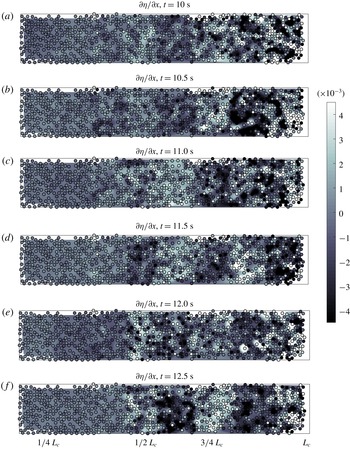
To measure perturbations in the slope of the water surface, we used an adaptation of the free-surface synthetic schlieren method (FS-SS) developed by Moisy, Rabaud & Salsac (Reference Moisy, Rabaud and Salsac2009). In our set-up, we track the apparent distortion of the circular tips of the submerged cylinders. Using particle tracking codes (Ouellette, Xu & Bodenschatz Reference Ouellette, Xu and Bodenschatz2006), the apparent displacement of the cylinder tips is measured over time and converted to the surface slope field. A full description and validation of this approach can be found in Mandel et al. (Reference Mandel, Rosenzweig, Chung, Ouellette and Koseff2017). A sample snapshot of the perturbations in streamwise surface slope is shown in figure 2; obvious quasi-two-dimensional structures are observable.
Snapshots of perturbations in streamwise surface slope over time for case 20A2. Black-edged circles indicate the location of the vegetation elements, and shading that fills the circles represents the streamwise surface slope
 $\unicode[STIX]{x2202}\unicode[STIX]{x1D702}/\unicode[STIX]{x2202}x$
. The surface slope is interpolated between elements to better show features. The horizontal axis indicates the streamwise direction
 $x$
, and vertical axis represents the transverse direction
 $y$
. Snapshots are of the centre 30 cm of a 60 cm wide test section. The apparent displacement of the tips of the cylindrical elements is very small, of the order of 1–2 pixels, so positions of the elements appear identical in all frames.

An array of eight Basler Ace (model number acA1300-60gm) monochrome cameras was set up to image the length of the cylinder array. Camera synchronization and image logging were performed using a LabVIEW program. Cameras were triggered by a function generator (BNC Model 555 Pulse/Delay Generator), and images were transferred by Ethernet cables onto two data acquisition computers. Camera frame rate was set to 10 frames per second, with all cameras taking images simultaneously. Each camera was equipped with a Tamron lens with an f-stop of F/2.1, focal length of 35 mm and exposure time of
 $12\,000~\unicode[STIX]{x03BC}\text{s}$
. Images were
 $1280\times 1024$
pixels, yielding a field of view (FOV) of approximately 30 cm
 $\times$
25 cm. The cameras were positioned 206 cm above the flume bottom.
In addition to the FS-SS measurements, we also collected two-component laser Doppler anemometry (LDA) measurements approximately 1 cm downstream of the end of the canopy so that the mean velocity, shear length scale and turbulence within the water column could be compared to surface measurements. The LDA system consists of a Laser Quantum Ventus 250 laser emitting at 532 nm, in conjunction with a Dantec optical assembly consisting of two beam splitters, two Bragg cells and focusing and receiving optics. For each experimental case, a vertical profile of seven points was taken: a free-stream measurement approximately 8 mm below the free surface; a ‘within-canopy’ measurement 3 cm above the bed; and five points measured within the canopy shear layer. At each point, horizontal and vertical velocities were recorded for 12 min at sampling rates of 500–1200 Hz, then filtered to a uniform sampling rate of 25 Hz.
The within-canopy and near-surface measurements are used to represent
 $U_{s}$
and
 $U_{c}$
, the asymptotic limits of the time-averaged mixing layer profile shown in figure 1. The vertical position to measure
 $U_{c}$
was chosen based on the profiles, with finer vertical resolution, of Rosenzweig (Reference Rosenzweig2017). From this, we concluded that the profile beneath
 $z=5$
cm above bed was relatively constant, to within
 $\pm 0.4~\text{cm}~\text{s}^{-1}$
. Similarly, the relative error in choosing a fixed point to represent
 $U_{s}$
is expected to be
 $\pm 1~\text{cm}~\text{s}^{-1}$
. These uncertainties are also considered when computing the velocity difference
 $\unicode[STIX]{x0394}U=U_{s}-U_{c}$
and depth-averaged velocity
 $\overline{U}=(U_{s}+U_{c})/2$
discussed in § 3.
2.3 Image processing
For these studies, a few additional postprocessing steps on the images were required. First, because of strong surface-impacting boils, some tracked cylinder tips towards the downstream edge of the canopy had discontinuous time series. These tracks were merged by clustering tracks into groups with the same mean [
 $X,Y$
] pixel location and linearly interpolating short gaps in the time record. Second, in a few experimental cases with the densest canopies, drag was high enough that the canopy itself moved during the experiments. While this shift was negligible from a physical standpoint, it did yield an overall drift in the streamwise pixel location of cylinder tips of the order of
 ${\leqslant}1$
pixel. This low-frequency trend was subtracted from the high-frequency deflections of interest by applying a median filter to the signal and subtracting the mean trend to yield a signal centred about zero.
3 Results
3.1 Vortex properties and connection to the bulk flow
Following the methods described in Mandel et al. (Reference Mandel, Rosenzweig, Chung, Ouellette and Koseff2017), we calculated the propagation speed, peak instability frequency and characteristic length scales of the vortices from their surface signal. The vortex velocity at the surface,
 $U_{v}$
, was computed using values of spatial distance
 $\unicode[STIX]{x0394}x$
between two signals and their associated correlation peak in time
 $\unicode[STIX]{x0394}t$
. These values were computed along the centreline of the flume, and
 $U_{v}$
was computed as the slope of a fit to a plot of
 $\unicode[STIX]{x0394}x$
versus
 $\unicode[STIX]{x0394}t$
.
In figure 3, the vortex speed at the surface is compared with two subsurface flow properties: the mean velocity at the canopy height,
 $U_{h_{c}}$
; and a representation of the depth-averaged velocity,
 $$\begin{eqnarray}\overline{U}=\frac{U_{s}+U_{c}}{2},\end{eqnarray}$$
where
 $U_{s}$
is the time-averaged velocity near the free surface and
 $U_{c}$
is the time-averaged within-canopy velocity. The vortex speed is linearly proportional to the depth-averaged flow velocity
 $\overline{U}$
. It is also representative of the velocity at
 $z=h_{c}\approx h_{i}$
, the mean velocity at the canopy height and at the slightly raised inflection point of the velocity profile. Thus, the vortex speed at the surface is reflective of bulk flow properties and the shear that induces this instability. This agrees well with previous observations in both terrestrial and aquatic canopies (Finnigan Reference Finnigan1979; Ghisalberti & Nepf Reference Ghisalberti and Nepf2002), as well as previous work in idealized free shear layers (Ho & Huerre Reference Ho and Huerre1984).
Vortex speed, as measured at the surface, for varying canopy height, density and flow speed. Measurements at the free surface are compared to LDA measurements of depth-averaged velocity
 $\overline{U}$
and
 $U_{h_{c}}$
. It is apparent that the speed of the vortex at the free surface is a sufficient analogue for common representations of the shear layer velocity.

Nepf (Reference Nepf2011) noted that in a canopy shear layer, vortices are displaced upward relative to the canopy due to the canopy drag, and that as a result, the translation speed of the vortices is higher than the velocity at the inflection point. Ghisalberti & Nepf (Reference Ghisalberti and Nepf2002) observed that the velocity ratio
 $U_{v}/U_{h_{c}}$
increased with increasing depth of submergence (
 $H/h_{c}$
), with a value of
 $U_{v}/U_{h_{c}}=1.8$
observed at
 $H/h_{c}=4.5$
. Nepf (Reference Nepf2011) suggests that this value is the asymptotic limit for unconfined canopies, as
 $U_{v}/U_{h_{c}}$
is also 1.8 in terrestrial canopies (Finnigan Reference Finnigan1979). As shown in figure 4, we found a maximum velocity ratio around 1.8 for more strongly submerged canopies. However, we also observed significant spread due to the canopy density at different submergence ratios. The velocity ratio is highest for the densest canopy case, indicating that vortex centres are more significantly displaced upwards when the canopy is providing more resistance and restricting within-canopy flow.
We also examined two metrics of the physical vortex scale, based on the spatial correlation function:
 $$\begin{eqnarray}R_{xx}(r,x)=\left\langle \frac{\unicode[STIX]{x2202}\unicode[STIX]{x1D702}}{\unicode[STIX]{x2202}x}(x,t)\cdot \frac{\unicode[STIX]{x2202}\unicode[STIX]{x1D702}}{\unicode[STIX]{x2202}x}(x+r,t)\right\rangle ,\end{eqnarray}$$
where angle brackets represent a time average. Evaluating this function at any given downstream location
 $x$
, we found both the value of
 $r$
at which the function (i) first crosses zero, i.e. a decorrelation length; and (ii) reaches its second correlation peak. We define the first as a representation of the vortex size
 $L_{v}$
and the second as a representation of the streamwise vortex spacing or wavelength
 $\unicode[STIX]{x1D706}_{v}$
.
Ratio of vortex velocity to velocity at the canopy height as a function of submergence ratio. The velocity ratio is highest for the densest canopy case (black circles), indicating that vortex centres are more significantly displaced upwards when the relative porosity of the canopy is lower. The dashed line at
 $U_{v}/U_{h_{c}}=1.8$
indicates the asymptotic limit postulated by Nepf (Reference Nepf2011).

Figure 5 shows these two length scales as a function of downstream distance. Once a coherent signal has emerged at the free surface, the vortex size stays approximately constant with downstream distance. The vortex spacing, however, grows at a constant rate. The predominant instability frequency, shown in figure 5(b), also changes at a constant rate with downstream distance. This behaviour is seen for all experimental cases and will be examined more closely in § 3.4.
Figure 6 compares the two surface vortex length scales
 $L_{v}$
and
 $\unicode[STIX]{x1D706}_{v}$
against the canopy height
 $h_{c}$
. The vortex size shown is the median value over the region of the canopy where
 $x/L_{c}>0.55$
, i.e. where a surface signature is significant and relatively coherent for all cases. The vortex spacing shown is the median of the last three measurements at the end of the canopy, so that these end-canopy surface measurements can be compared with end-canopy velocity measurements. The vortex size is inversely proportional to the canopy height. While previous work found that vortex size scales directly with
 $h_{c}$
, these results show that instead the vortex size decreases with increasing canopy height – at least for the more strongly confined flows studied here. This suggests that there is some submergence limit beyond which the dominant turbulent length scale is
 $H-h_{c}$
, the distance between the top of the canopy and the free surface. Previous studies have generally normalized the measured vortex length scales by the canopy height. Shown in figure 7 is a comparison of data from a number of previous studies of estimated vortex size as a function of submergence ratio. The data of Okamoto & Nezu (Reference Okamoto and Nezu2009) are comprised of the integral length scale at the canopy height for both flexible (open circles) and rigid (filled circles) vegetation. Okamoto et al. (Reference Okamoto, Nezu and Sanjou2016) also computed the integral length scale, but at the canopy height and near the surface. Finally, the data of Ghisalberti & Nepf (Reference Ghisalberti and Nepf2002) are estimates of vertical vortex size based on momentum thickness
 $\unicode[STIX]{x1D703}$
and mixing layer thickness
 $t_{ml}$
. Normalizing the vortex length scale
 $L_{x}$
(as defined in each study) by
 $(H-h_{c})$
yields a much better collapse (indicated by a more coherent trend in the data, not simply a reduction in the vertical spread of the data), particularly for the data of Ghisalberti & Nepf (Reference Ghisalberti and Nepf2002). This collapse also minimizes some of the variation due to canopy rigidity/flexibility. This result, that vortex size scales well with the canopy–surface gap
 $(H-h_{c})$
, agrees with some prior discussions in the literature; Nepf & Vivoni (Reference Nepf and Vivoni2000), for example, noted that for
 $H/h_{c}<2$
, penetration of turbulence into the canopy is depth limited.
Vortex length scales and predominant frequency at the free surface for case 20A1 versus distance downstream. (a) Length scales are normalized by the canopy height
 $h_{c}$
. A coherent signal emerges at the free surface around
 $x/L_{c}\sim 0.4$
, at which time spatial correlations become significant. The vortex size
 $L_{v}$
remains fairly fixed over the canopy length, while the vortex spacing
 $\unicode[STIX]{x1D706}_{v}$
grows at a constant rate. The vortex spacing has almost doubled by the end of the canopy. (b) The predominant frequency observed at the surface shows a similar linear trend with downstream distance. Shaded error bars indicate the order of magnitude of error in each measurement point.

The shear length scale
 $L_{s}$
is the dominant flow length scale (Raupach, Finnigan & Brunet Reference Raupach, Finnigan and Brunet1996; Finnigan Reference Finnigan2000):
 $$\begin{eqnarray}L_{s}=\frac{U_{z=h_{c}}}{\unicode[STIX]{x2202}U/\unicode[STIX]{x2202}z}_{z=h_{c}}.\end{eqnarray}$$
The vortex size and spacing are compared with the shear length scale
 $L_{s}$
in figure 8. While vortex size is uncorrelated with shear length, the vortex spacing has some correlation (
 $R^{2}=0.39$
) with the shear length scale. Raupach et al. (Reference Raupach, Finnigan and Brunet1996) found that in a terrestrial canopy, dominant eddies scaled with the shear length scale, and that the streamwise spacing
 $\unicode[STIX]{x1D706}_{v}$
of these eddies equalled
 $8.1L_{s}$
. Again, it seems that confined shear layers behave differently from the free shear layers of terrestrial flows. In our experiments, flows with stronger shear (and thus shorter shear length) have a larger vortex wavelength. The canopy geometry that generates the strongest shear is, as expected, the densest canopy. Thus, the frequency and wavelength of the structures shed from the canopy are related to the canopy density.
Vortex length scales as a function of canopy geometry. (a) The vortex size shows an inverse proportionality to the canopy height
 $h_{c}$
. While previous work found that in unconfined canopies, vortex size
 ${\sim}h_{c}$
, these results in more strongly submerged canopies find the inverse, that vortex size decreases for larger canopy heights;
 $h_{c}$
of 10 cm corresponds to a submergence ratio
 $H/h_{c}$
of 3.1, while
 $h_{c}$
of 20 cm corresponds to
 $H/h_{c}$
of 1.6. (b) The vortex spacing shows a similar dependence on the canopy height, in addition to dependence on the canopy density, here represented by the dimensionless planform density
 $\unicode[STIX]{x1D706}_{p}$
. Denser canopies generate a larger vortex spacing relative to sparser canopies.

Comparison of vortex size estimates from this study and previous studies. Data for rigid model vegetation are shown as filled symbols, and data for flexible vegetation as open symbols. The data of Okamoto & Nezu (Reference Okamoto and Nezu2009) are comprised of the integral length scale at the canopy height for both flexible and rigid vegetation. Okamoto et al. (Reference Okamoto, Nezu and Sanjou2016) also computed the integral length scale, but at the canopy height and near the surface. Finally, the data of Ghisalberti & Nepf (Reference Ghisalberti and Nepf2002) are estimates of vertical vortex size based on
 $\unicode[STIX]{x1D703}$
and
 $t_{ml}$
. The data for the present study are the vortex size estimates
 $L_{v}$
, based on the decorrelation length. Best fit lines in (b) show an exponential fit of the form
 $y=a\text{e}^{bx}$
for data from previous work (
 $a=5.5$
,
 $b=-0.71$
), and all work including the data from the present study (
 $a=2.5$
,
 $b=-0.48$
).

Shear length scale versus vortex length and spacing. (a) The shear length scale shows very little correlation with the vortex size at the surface. (b) The shear length correlates reasonably well with the vortex spacing at the end of the canopy. A linear relation is found with
 $R^{2}=0.39$
.

3.2 Stability of measured velocity profiles
Ghisalberti & Nepf (Reference Ghisalberti and Nepf2002) used a mixing layer model for a canopy velocity profile:
 $$\begin{eqnarray}\frac{U-\overline{U}}{\unicode[STIX]{x0394}U}=\frac{1}{2}\tanh \left(\frac{z-\overline{z}}{2\unicode[STIX]{x1D703}}\right),\end{eqnarray}$$
where
 $\overline{z}$
is a reference height such that
 $(z-\overline{z})/\unicode[STIX]{x1D703}$
at the inflection point. Rearranging to obtain
 $U$
as a function of depth,
 $$\begin{eqnarray}U(z)=\frac{1}{2}\unicode[STIX]{x0394}U\tanh \left(\frac{z-h_{i}}{2\unicode[STIX]{x1D703}}\right)+\overline{U}.\end{eqnarray}$$
In canopy shear layers, the inflection point of the velocity profile is shifted upwards from the actual canopy height. Because this shift was not known a priori, to compute this correction to the location of the inflection point, we ran a nonlinear optimization algorithm to fit (3.5) to all 27 measured velocity profiles, with
 $h_{i}$
as a free variable. The effect of this correction in more accurately capturing the measured behaviour can be seen in figure 9. Both models in the figure use values of
 $\unicode[STIX]{x0394}U$
(
 $=U_{s}-U_{c}$
),
 $\unicode[STIX]{x1D703}$
and
 $\overline{U}$
from subsurface measurements. Following Ghisalberti & Nepf (Reference Ghisalberti and Nepf2002) and Rosenzweig (Reference Rosenzweig2017), who found that the momentum thickness
 $\unicode[STIX]{x1D703}$
scales with the mixing layer thickness
 $t_{ml}$
(
 $t_{ml}/\unicode[STIX]{x1D703}=7.1\pm 0.4$
and
 $t_{ml}/\unicode[STIX]{x1D703}=6.7\pm 0.4$
, respectively), we computed the momentum thickness as
 $$\begin{eqnarray}\unicode[STIX]{x1D703}=\frac{t_{ml}}{7}=\frac{H-(h_{c}-\unicode[STIX]{x1D6FF}_{e})}{7}.\end{eqnarray}$$
Following the derivation of the penetration depth in Nepf (Reference Nepf2011), the penetration depth
 $\unicode[STIX]{x1D6FF}_{e}$
is approximated as being equal to the measured shear length scale
 $L_{s}$
.
Correction of the inflection point height
 $h_{i}$
for sample velocity profiles 20A1, 15A1 and 10A1. Black circles indicate mean velocities measured using LDA. The solid blue line shows the model of
 $U(z)$
using the canopy height as the location of inflection. The dot-dashed black line shows (3.5), where a corrected inflection height has been fitted from the data. Both models use values of
 $\unicode[STIX]{x0394}U$
,
 $\unicode[STIX]{x1D703}$
and
 $\overline{U}$
from subsurface measurements. The horizontal dotted line indicates the canopy height.

Our measurements of the canopy velocity profiles indicated that for every case, there is an inflection point making the flow susceptible to Kelvin–Helmholtz instability. We thus conducted a linear instability analysis to understand the most unstable modes generated by these profiles. As discussed in Raupach et al. (Reference Raupach, Finnigan and Brunet1996), linear stability theory ceases to apply as soon as the instabilities grow to a finite size; however, the analysis is informative in identifying the amplified modes that should dominate the flow.
To assess the stability of these velocity profiles, we followed the methods of Biancofiore et al. (Reference Biancofiore, Heifetz, Hoepffner and Gallaire2017), which we will summarize here. First we began with the non-dimensionalized, two-dimensional Navier–Stokes equations linearized about the mean flow profile
 $U(z)$
:
 $$\begin{eqnarray}\displaystyle & \displaystyle \frac{\unicode[STIX]{x2202}u}{\unicode[STIX]{x2202}t}+U\frac{\unicode[STIX]{x2202}u}{\unicode[STIX]{x2202}x}+w\frac{\unicode[STIX]{x2202}U}{\unicode[STIX]{x2202}z}=-\frac{\unicode[STIX]{x2202}p}{\unicode[STIX]{x2202}x}+\frac{1}{Re}\unicode[STIX]{x1D6FB}^{2}u, & \displaystyle\end{eqnarray}$$
 $$\begin{eqnarray}\displaystyle & \displaystyle \frac{\unicode[STIX]{x2202}w}{\unicode[STIX]{x2202}t}+U\frac{\unicode[STIX]{x2202}w}{\unicode[STIX]{x2202}x}=-\frac{\unicode[STIX]{x2202}p}{\unicode[STIX]{x2202}z}+\frac{1}{Re}\unicode[STIX]{x1D6FB}^{2}w. & \displaystyle\end{eqnarray}$$
And continuity,
 $$\begin{eqnarray}\frac{\unicode[STIX]{x2202}u}{\unicode[STIX]{x2202}x}+\frac{\unicode[STIX]{x2202}w}{\unicode[STIX]{x2202}z}=0.\end{eqnarray}$$
These equations can be written in operator form as:
 $$\begin{eqnarray}0=\left(-\left[\begin{array}{@{}ccc@{}}\unicode[STIX]{x2202}_{t} & 0 & 0\\ 0 & \unicode[STIX]{x2202}_{t} & 0\\ 0 & 0 & 0\end{array}\right]+\left[\begin{array}{@{}ccc@{}}-U\unicode[STIX]{x2202}_{x}+\frac{I}{Re}\unicode[STIX]{x1D6FB}^{2} & U_{z} & -\unicode[STIX]{x2202}_{x}\\ 0 & -U\unicode[STIX]{x2202}_{x}+\frac{I}{Re}\unicode[STIX]{x1D6FB}^{2} & -\unicode[STIX]{x2202}_{z}\\ \unicode[STIX]{x2202}_{x} & \unicode[STIX]{x2202}_{z} & 0\end{array}\right]\right)\left[\begin{array}{@{}c@{}}u\\ w\\ p\end{array}\right].\end{eqnarray}$$
We decomposed the solutions
 $u$
,
 $w$
and
 $p$
into normal modes, assuming oscillating behaviour in
 $x$
and time:
 $$\begin{eqnarray}u=\hat{u} (z)\text{e}^{\text{i}(kx-\unicode[STIX]{x1D714}t)},\end{eqnarray}$$
where
 $\hat{u}$
is the amplitude function of
 $u$
as a function of
 $z$
,
 $k$
is the streamwise spatial wavenumber and
 $\unicode[STIX]{x1D714}$
is the temporal oscillation frequency. Similar equations were made for
 ${\hat{w}}$
and
 $\hat{p}$
. The derivative operators in (3.10) can now be expressed in terms of
 $\unicode[STIX]{x1D714}$
and
 $k$
(i.e.
 $\unicode[STIX]{x2202}_{t}=-\text{i}\unicode[STIX]{x1D714}$
,
 $\unicode[STIX]{x2202}_{x}=\text{i}k$
):
 $$\begin{eqnarray}\displaystyle 0 & = & \displaystyle \left(-\unicode[STIX]{x1D714}\underbrace{\left[\begin{array}{@{}ccc@{}}-\text{i} & 0 & 0\\ 0 & -\text{i} & 0\\ 0 & 0 & 0\end{array}\right]}_{E}\right.\nonumber\\ \displaystyle & & \displaystyle \left.+\,\overbrace{\underbrace{\left[\begin{array}{@{}ccc@{}}{\displaystyle \frac{I}{Re}}\unicode[STIX]{x2202}_{zz} & U_{z} & 0\\ 0 & {\displaystyle \frac{I}{Re}}\unicode[STIX]{x2202}_{zz} & -\unicode[STIX]{x2202}_{z}\\ 0 & \unicode[STIX]{x2202}_{z} & 0\end{array}\right]}_{\unicode[STIX]{x1D608}_{00}}+\,k\underbrace{\left[\begin{array}{@{}ccc@{}}-U\text{i} & 0 & -\text{i}\\ 0 & -U\text{i} & 0\\ \text{i} & 0 & 0\end{array}\right]}_{\unicode[STIX]{x1D608}_{1}}+\,k^{2}\underbrace{\left[\begin{array}{@{}ccc@{}}-I/Re & 0 & 0\\ 0 & -I/Re & 0\\ 0 & 0 & 0\end{array}\right]}_{\unicode[STIX]{x1D608}_{2}}}^{A}\right)\nonumber\\ \displaystyle & & \displaystyle \times \,\underbrace{\left[\begin{array}{@{}c@{}}\hat{u} \\ {\hat{w}}\\ \hat{p}\end{array}\right]}_{\hat{\boldsymbol{q}}}.\end{eqnarray}$$
This equation is a dispersion relation: if
 $k$
is given,
 $\unicode[STIX]{x1D714}$
is the eigenvalue of the generalized eigenvalue problem
 $$\begin{eqnarray}\unicode[STIX]{x1D714}\unicode[STIX]{x1D640}\hat{\boldsymbol{q}}=\unicode[STIX]{x1D63C}\hat{\boldsymbol{q}},\end{eqnarray}$$
where
 $\unicode[STIX]{x1D63C}$
is the matrix shown above in (3.12). This equation is solved numerically for the unstable eigenvalues. The Chebyshev differentiation matrices in
 $\unicode[STIX]{x1D608}_{00}$
were generated using the MATLAB differentiation matrix suite developed by Weideman & Reddy (Reference Weideman and Reddy2000). Neumann boundary conditions (no flux, no stress) were used at the bottom (
 $z=0$
) and top (
 $z=H$
) of the domain.
Given a Reynolds number
 $Re=\unicode[STIX]{x0394}U\unicode[STIX]{x1D703}/\unicode[STIX]{x1D708}$
, we took the dimensional base profile defined in (3.5) and non-dimensionalized with
 $U=(\unicode[STIX]{x0394}U)U^{\ast }$
and
 $z=\unicode[STIX]{x1D703}z^{\ast }$
. The base profile which was inserted into (3.12) (with dropped
 $^{\ast }$
) is thus
 $$\begin{eqnarray}U^{\ast }(z^{\ast })=\frac{1}{2}\tanh \left(\frac{z^{\ast }}{2}-\frac{h_{i}}{2\unicode[STIX]{x1D703}}\right)+\frac{\overline{U}}{\unicode[STIX]{x0394}U}\end{eqnarray}$$
and the first derivative of the base profile with respect to
 $z^{\ast }$
is
 $$\begin{eqnarray}\frac{\unicode[STIX]{x2202}U^{\ast }}{\unicode[STIX]{x2202}z^{\ast }}=\frac{1}{4}\cosh \left(\frac{z^{\ast }}{2}-\frac{h_{i}}{2\unicode[STIX]{x1D703}}\right)^{-2}.\end{eqnarray}$$
We have focused here on the temporal problem. Using the measurements of vortex wavelength at the free surface, we defined a non-dimensional wavenumber
 $k$
(
 $k=2\unicode[STIX]{x03C0}\unicode[STIX]{x1D703}/\unicode[STIX]{x1D706}_{v}$
) to find non-dimensional frequency
 $\unicode[STIX]{x1D714}$
. We solved the eigenvalue problem defined in (3.13) and found the one unstable eigenmode. For the temporal case, the unstable eigenvalue is that which has a positive imaginary component, e.g. for a given
 $k$
and complex eigenvalue
 $\unicode[STIX]{x1D714}=\unicode[STIX]{x1D714}_{r}+\text{i}\unicode[STIX]{x1D714}_{i}$
,
 $$\begin{eqnarray}\text{e}^{-\text{i}\unicode[STIX]{x1D714}t}=\text{e}^{-\text{i}(\unicode[STIX]{x1D714}_{r}+\text{i}\unicode[STIX]{x1D714}_{i})t}=\underbrace{(\text{e}^{-\text{i}\unicode[STIX]{x1D714}_{r}t})}_{Real\,\rightarrow \,oscillation}\ast \overbrace{(\text{e}^{\unicode[STIX]{x1D714}_{i}t})}^{Positive\,imaginary\,\rightarrow \,growth}.\end{eqnarray}$$
The unstable eigenmode for each velocity profile is shown in figure 10. Colour bars show non-dimensional planform area
 $\unicode[STIX]{x1D706}_{p}$
, a representation of canopy density. Canopies with the highest density experience faster growth rates of the instability, and shed vortices at a lower frequency. The slope of figure 10(b) represents the propagation speed of the vortices,
 $\unicode[STIX]{x1D714}_{r}/k=\overline{U}/\unicode[STIX]{x0394}U\approx 0.7$
.
Non-dimensional growth rate and oscillation frequency as a function of wavenumber for all 27 experimental cases. Colour bars show non-dimensional planar density parameter
 $\unicode[STIX]{x1D706}_{p}$
, a representation of canopy density. Canopies with the highest density experience faster growth rates of the instability, and shed vortices at a lower frequency.

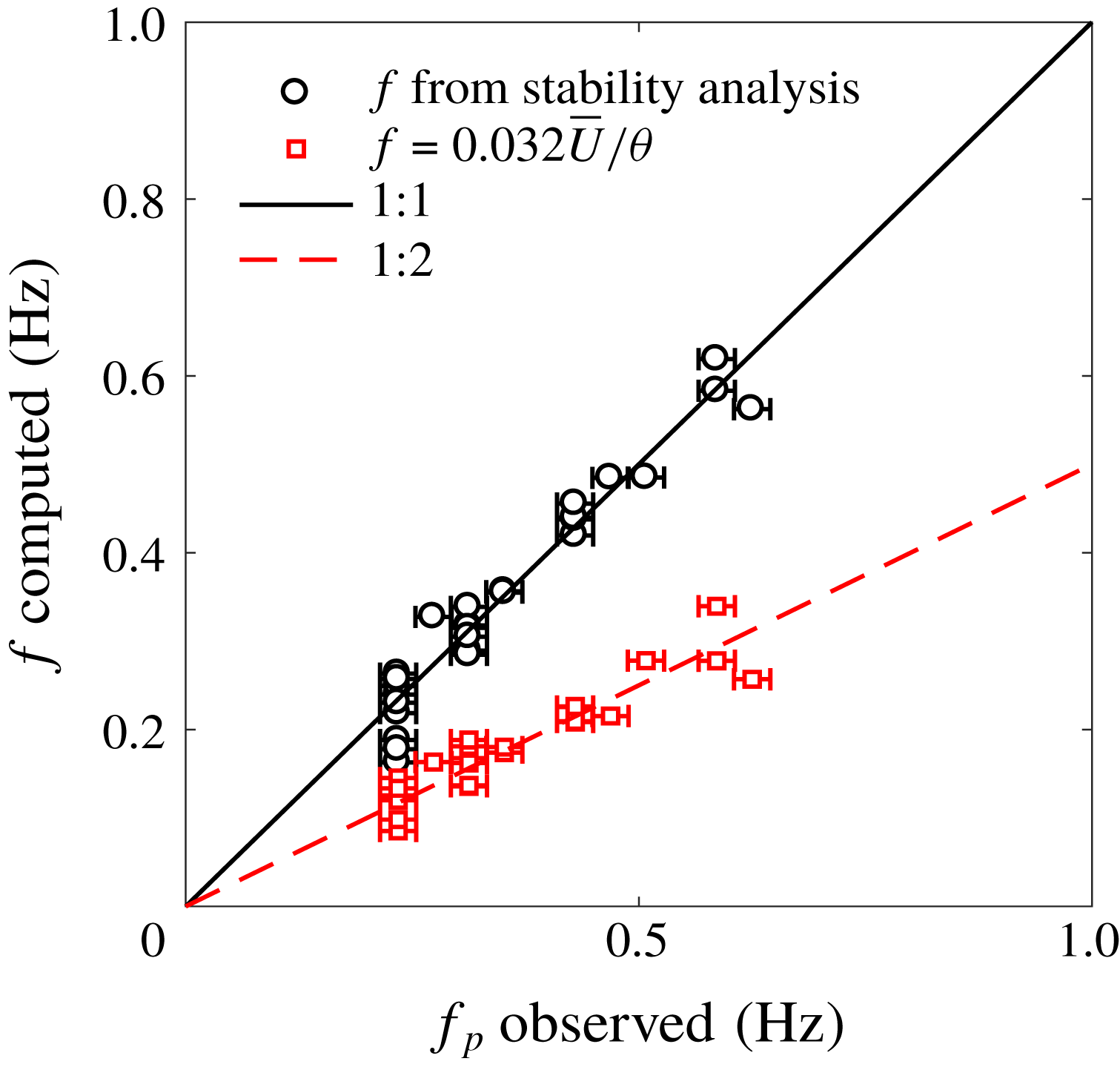
Observed instability frequency from measured surface slope spectrum versus computed values of the instability frequency, given measured instability wavelengths. Black circles show the unstable mode computed in the above analysis. Red squares show the commonly used Strouhal shedding frequency defined in Ho & Huerre (Reference Ho and Huerre1984).
Non-dimensional instability growth rate versus range of Strouhal numbers for three sample velocity profiles. Lines indicate the theoretical growth rate of the most unstable mode for a range of forcing wavenumbers/frequencies. Shaded region indicates the relative frequency of occurrence of experimentally observed Strouhal numbers, with darker regions indicating the most common
 $St$
.

We can compare the dimensional frequency computed in this stability analysis (
 $f=(\unicode[STIX]{x0394}U/2\unicode[STIX]{x03C0}\unicode[STIX]{x1D703})\unicode[STIX]{x1D714}_{r}$
) with the peak frequency observed in the spectra of surface slope,
 $f_{p}$
, again as measured at the downstream end of the canopy. Figure 11 shows these two quantities, as well as the Strouhal shedding frequency (
 $f=0.032\overline{U}/\unicode[STIX]{x1D703}$
) defined in Ho & Huerre (Reference Ho and Huerre1984) and observed in Ghisalberti & Nepf (Reference Ghisalberti and Nepf2002), Nezu & Sanjou (Reference Nezu and Sanjou2008), Okamoto & Nezu (Reference Okamoto and Nezu2009) and Okamoto et al. (Reference Okamoto, Nezu and Sanjou2016). While solving the dispersion relation given the observed wavelengths yields agreement with our experimentally measured frequencies, these observed frequencies do not agree with
 $f=0.032\overline{U}/\unicode[STIX]{x1D703}$
previously shown in the literature.
Based on our surface slope spectra, we instead observed a Strouhal number closer to twice the classical value of 0.032 cited from Ho & Huerre (Reference Ho and Huerre1984), with
 $St$
ranging from 0.05 to 0.08 and a mean of
 $St=0.064$
. For three sample velocities profiles, the dispersion relation was next solved given a wide range of forcing wavenumbers. Figure 12 shows this range of observed Strouhal numbers in comparison with the results of our linear stability analysis in determining the most amplified wave. The maximum theoretical growth rate occurs for
 $St=0.032$
, while the shaded region indicates the relative occurrence of actual observed Strouhal shedding frequencies, with the average centred about twice the most amplified
 $St$
.
As noted in the review of Ho & Huerre (Reference Ho and Huerre1984), the Strouhal number of the most amplified wave corresponds to the natural frequency of the mixing layer; the most unstable mode at
 $St=0.032$
may indeed be representative of the local instability at the shear layer at the top of the canopy. It is possible that we are observing a transformation of shedding frequency between the top of the canopy and the free surface, the reasons for which warrant additional work beyond the scope of this paper. One possible explanation is nonlinear vortex-pairing or vortex-breakup interactions occurring between the generation of vortices at the canopy height (where previous measurements in the literature have focused), and the point at which vortices manifest at the free surface.
Ghisalberti & Nepf (Reference Ghisalberti and Nepf2004) also reported agreement with Ho & Huerre (Reference Ho and Huerre1984), and further assert that while there is a clear frequency peak inside the shear layer, there is not one outside – which conflicts with our findings here and those presented in Rosenzweig (Reference Rosenzweig2017). While Ghisalberti & Nepf (Reference Ghisalberti and Nepf2004) interpret their findings as indicating that shear kinetic energy is not transported outside the shear layer, the presence of a clear surface signature, which agrees with our linear stability analysis, indicates that kinetic energy produced in the shear layer has a strong influence at the free surface. This work thus has important implications for the role of aquatic vegetation in air–sea gas exchange as well.
Parameterization of interior flow variables with surface variables.

3.3 Reconstructing velocity profiles from surface measurements
Given these surface measurements of vortex size, spacing, speed and frequency, another question arises: How predictive are surface measurements of the interior flow? Can surface measurements be used to reconstruct a full velocity profile?
Cornelisen & Thomas (Reference Cornelisen and Thomas2004, Reference Cornelisen and Thomas2006) and others have shown that nutrient uptake rate within seagrass communities is strongly dependent upon current velocity and Reynolds stress at the canopy height. Because of the complexity of canopy velocity profiles, near-surface velocity measurements are not adequate to predict within-canopy velocities or bulk, depth-averaged quantities. Thus, being able to accurately predict the velocity both above and within vegetation from remote sensing measurements would be advantageous to ecologists. Beyond velocities, Orth, Luckenbach & Moore (Reference Orth, Luckenbach and Moore1994) showed that one primary predictor of particle transport downstream of a submerged canopy is the canopy height (i.e. the height at which a seed or propagule is released). Thus, understanding where in the water column the region of seed release occurs, and what velocities that seed is subjected to, may be indicative of how far seeds and sediment may be transported or where scour may be particularly strong.
The velocity profile defined by (3.5) is a function of
 $\unicode[STIX]{x0394}U$
,
 $h_{i}$
,
 $\unicode[STIX]{x1D703}$
and
 $\overline{U}$
. These values are all correlated with measurements at the free surface, suggesting that a model for the velocity profile may be constructed based on parameterizations of surface measurements. These linear fits are shown in figure 13, and the equations are summarized in table 2. The equations in this table can then be substituted into (3.5) to allow for prediction of
 $U(z)$
simply from surface measurements of
 $U_{v}$
and
 $L_{v}$
.
The primary limitation of this approach is that knowledge of the water depth
 $H$
is required. Additionally, while a simple linear fit to predict
 $\unicode[STIX]{x0394}U$
as a function of
 $U_{v}$
is possible, including the canopy density in the parameterization would increase the accuracy of this prediction and capture more of the spread in
 $\unicode[STIX]{x0394}U$
. However, we have not found a surface-based parameter that is directly predictive of canopy density, so we did not include this refinement in the analysis.
Figure 14 shows the performance of the surface model parameterization versus LDA data for the intermediate Reynolds number case. Shown with the black dot-dashed line is the hyperbolic tangent model of (3.5) using inputs based on LDA data, and an optimized inflection point height. The dashed red line represents the hyperbolic tangent model using inputs based solely on surface measurements using FS-SS. The surface-based model performs reasonably well in predicting the measured velocity profile, with the main error occurring (as expected based on figure 13) in predictions of
 $\unicode[STIX]{x0394}U$
, the difference between the free-stream and within-canopy velocities.
Correlation of surface measurements with interior flow measurements to obtain parameterizations for the velocity profile, equation (3.5). While in (a), (c) and (d), all densities are plotted as black circles, (b) shows how scatter in
 $\unicode[STIX]{x0394}U$
is a function of canopy density
 $\unicode[STIX]{x1D706}_{P}$
. We expect this single linear fit to perform best for the intermediate density,
 $\unicode[STIX]{x1D706}_{P}=0.08$
.

Performance of surface model parameterization versus LDA data for the intermediate Reynolds number case. Black circles represent velocity measurements taken using LDA. The canopy height is indicated by the light dashed horizontal line. The dot-dashed black line represents the hyperbolic tangent model of (3.5) using inputs based on LDA data, and an optimized inflection point height. The dashed red line represents the hyperbolic tangent model using inputs based solely on surface measurements using FS-SS. The surface-based model performs reasonably well in predicting the measured velocity profile, with the main error occurring in predictions of
 $\unicode[STIX]{x0394}U$
, the difference between the free-stream and within-canopy velocities.

To quantitatively assess the goodness of fit, the normalized root-mean-squared error for each case is computed as
 $$\begin{eqnarray}\text{RMSE}=\frac{1}{\unicode[STIX]{x0394}U}\sqrt{\frac{1}{N}\mathop{\sum }_{i=1}^{N}(U_{i,data}-U_{i,model})^{2}},\end{eqnarray}$$
where
 $i=1$
to
 $N$
are points in each measured vertical velocity profile and
 $N=7$
is the number of vertical measurements. The error is plotted against the non-dimensional canopy frontal area
 $\unicode[STIX]{x1D706}_{f}$
in figure 15. The surface model performs reasonably well, with RMSE
 ${\leqslant}10\,\%$
for the majority of the cases. The largest error occurs for the lowest
 $Re$
cases.
Performance of surface model parameterization versus measured values for all experimental cases. The root-mean-squared error for each case, normalized by
 $\unicode[STIX]{x0394}U$
, is plotted against the non-dimensional canopy frontal area
 $\unicode[STIX]{x1D706}_{f}$
. The model performs reasonably well, with RMSE
 ${\leqslant}10\,\%$
for the majority of the cases. The largest error occurs for the lowest
 $Re$
cases.

We thus are able to predict the velocity profile where
 $U(z)=f(z,H,U_{v},L_{v})$
. In other words, if the local water depth is known, and spatially and temporally resolved surface measurements can be taken, then a reasonable estimate of the subsurface velocity profile is possible, including important interior flow parameters such as within-canopy velocities and inflection point of the profile. As mentioned before, these parameters are useful to estimates of nutrient uptake and seed dispersal by aquatic plants.
3.4 Streamwise evolution of the vortices
While we have been able to measure consistent bulk flow parameters from these surface measurements, the streamwise evolution of the surface signal also provides an interesting opportunity for exploration.
First, we examined the spectral evolution of the instability signal. One might expect the power spectral density at the predominant instability frequency to grow with distance downstream, then reach some constant value once the flow has adjusted to the canopy drag and a fixed mean velocity profile has developed. Instead, we see a different behaviour at the end of the canopy, as demonstrated in figure 16, which plots the power spectral density at the measured peak instability frequency versus downstream distance for all experimental cases. The ratio between the distance to a peak in power spectral density
 $L_{PSD}$
and the vortex wavelength (
 $L_{PSD}/\unicode[STIX]{x1D706}_{v}$
) ranges from approximately 3 to 5. According to Ho & Huerre (Reference Ho and Huerre1984), for a Kelvin–Helmholtz wave and its harmonic, a peak and subsequent roll-off in the energy integral of the natural frequency wave occurs at approximately
 $X/\unicode[STIX]{x1D706}\approx 4$
. This suggests that the length scale of evolution we are observing is not unreasonable.
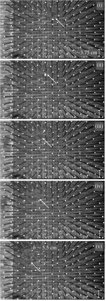
In several of the cases where a significant local maximum in power spectral density occurs, strong surface-impacting ‘boils’ were visually observed towards the end of the canopy. An example of such a structure can be seen in figure 17. These boils indicated increased cross-stream variability at the surface, as well as significant upwelling velocities. Beyond capillary wave generation by impinging eddies, one possible explanation for the loss in power spectral density in figure 16 is the transition from two-dimensional rollers to three-dimensional vortices.
Power spectral density at the measured peak instability frequency versus downstream distance
 $x/L_{c}$
for all experimental cases. Rows show differing canopy heights, and columns show different flow speeds. Markers indicate the canopy density. The densest canopy generates the most power at the instability frequency. Note the significant dropoff in power that occurs for many cases between
 $x/L_{c}=0.5$
and 1.

Images of a representative ‘boil’ structure impacting the free surface and propagating downstream (from right to left) towards the trailing edge of the canopy for experimental case 20A2. The side wall of the flume is in the lowermost portion of the images; the boil structure at the top of the image is approximately 30 cm from the side wall, moving along the centreline of the flume. By image (v), the centre boil structure is approximately 5.5 cm in diameter. The circumference of the primary upwelling structure is marked with a dotted circle. Small waves can be seen radiating away from the centre of the structure, causing optical distortion beyond its edges, so that the area of disturbed fluid is larger than the boil itself. Note that these photos were taken with a wider-angle lens than those used for actual FS-SS measurements. The arrow points to the region of lensing due to surface disturbance.

A schematic view of this transition was postulated by Finnigan, Shaw & Patton (Reference Finnigan, Shaw and Patton2009) from a large-eddy simulation study of a terrestrial canopy. Following the initial Kelvin–Helmholtz roll-up and development of transverse instability, the authors observed a characteristic eddy consisting of an upstream head-down sweep-generating hairpin vortex superimposed on a downstream head-up ejection-generating hairpin. This formation of a dual-hairpin eddy, or similar structure, could explain both the approximate doubling of the vortex spacing (shown in figure 5), as well as the upward pumping of fluid from the head-up ejection-generating hairpin. Another hypothetical view is that of Bailey & Stoll (Reference Bailey and Stoll2016), who saw smaller three-dimensional vortex structures superimposed on the two-dimensional rollers as plant canopy flow developed.
To get a heuristic view of whether this dynamics may be at play in our aquatic canopy, we postulated that the streamwise location of the local maximum occurring in figure 16 may be the distance at which eddies begin having a significant interaction with the free surface. Chickadel et al. (Reference Chickadel, Horner-Devine, Talke and Jessup2009) observed the surface manifestation of boils generated by a submerged sill, and modelled their behaviour using a vertical boil propagation model. The authors posited that the boils observed were the expression of a three-dimensional hairpin vortex, and that their upward propagation could be explained as the self-advection of a vortex dipole. Following Batchelor (Reference Batchelor1967), they defined the upward velocity of the vortex loop as
 $$\begin{eqnarray}w_{v}=\frac{\unicode[STIX]{x1D6E4}_{v}}{2\unicode[STIX]{x03C0}b},\end{eqnarray}$$
where
 $w_{v}$
is the upward velocity of the vortex loop,
 $\unicode[STIX]{x1D6E4}_{v}$
is the circulation of the vortex pair and
 $b$
is the distance between vortex pair centres. Chickadel et al. (Reference Chickadel, Horner-Devine, Talke and Jessup2009) used the lateral scale of the boils at the surface as a metric for this distance between vortex pair centres
 $b$
, assuming that this surface scale was approximately equal to the depth of the sill-induced shear layer. The circulation of each individual vortex in the pair is defined as the integral of vorticity
 $\unicode[STIX]{x1D714}$
over the vortex cross-section
 $\text{d}A$
,
 $$\begin{eqnarray}\unicode[STIX]{x1D6E4}_{v}=\int \unicode[STIX]{x1D714}\,\text{d}A\approx \unicode[STIX]{x1D714}\unicode[STIX]{x03C0}\left(\frac{b}{2}\right)^{2}.\end{eqnarray}$$
We assume that vorticity is primarily generated by the canopy and that mean cross-stream and vertical velocities are zero, so that
 $\unicode[STIX]{x1D714}\approx \unicode[STIX]{x2202}U/\unicode[STIX]{x2202}z$
. We approximate the shear in terms of the bulk flow parameters
 $\unicode[STIX]{x0394}U$
and
 $H-h_{c}$
, yielding
 $$\begin{eqnarray}\unicode[STIX]{x1D6E4}_{v}=\frac{\unicode[STIX]{x0394}U\unicode[STIX]{x03C0}}{H-h_{c}}\left(\frac{b}{2}\right)^{2}.\end{eqnarray}$$
Substituting into the vertical vortex velocity equation (3.18),
 $$\begin{eqnarray}w_{v}=\frac{1}{8}\frac{\unicode[STIX]{x0394}Ub}{H-h_{c}}.\end{eqnarray}$$
Using this value of the vertical vortex velocity, the downstream eruption point – that is, the distance from vortex generation to manifestation at the free surface – is found as
 $L_{1}=U(H-h_{c})/w_{v}$
. Using representative bulk flow measurements, we obtain the expression
 $$\begin{eqnarray}L_{1}=\frac{8(H-h_{c})^{2}}{b}\frac{\overline{U}}{\unicode[STIX]{x0394}U}.\end{eqnarray}$$
Here,
 $\overline{U}$
,
 $\unicode[STIX]{x0394}U$
and
 $H-h_{c}$
are known from LDA measurements. For case 20A2, boils at the surface were observed to have a diameter of approximately 5.5 cm (see figure 17). Robust quantitative information about the diameter of the boils and their dependence on canopy parameters is more difficult to obtain, as this was not the intent of the initial experiment design. However, we can use this order of magnitude as a starting point to examine how downstream distance to the local maximum in the power spectral density,
 $L_{PSD}$
, compares with the Chickadel et al. (Reference Chickadel, Horner-Devine, Talke and Jessup2009) model of
 $L_{1}$
. A comparison is shown in figure 18 for the two taller canopy heights,
 $h_{c}=20$
and 15 cm, as only one of 9 cases with the shortest canopy experienced a local maximum. Figure 18(a) shows estimates of
 $L_{1}$
using a single-value estimate of
 $b=5.5$
cm. Figure 18(b) shows the estimate when allowing
 $b$
to vary for different canopy heights to force a 1:1 relationship.
Distance to vortex–surface interaction. (a) PSD dropoff distance
 $L_{PSD}$
versus estimated boil eruption point
 $L_{1}$
computed using naive single-value estimate of boil diameter
 $b$
. (b)
 $L_{1}$
computed using fitted canopy height-dependent estimate of boil diameter. Dashed lines indicate a 1:1 correspondence.

This result suggests that canopies with smaller submergence ratios may produce smaller boil expressions at the surface. Chickadel et al. (Reference Chickadel, Horner-Devine, Talke and Jessup2009) found that the lateral scale of boils observed at the water surface was similar to the depth of the shear layer. If this is true, then variation in boil size may be correlated with the measured shear length scale and vortex spacing as well. Further research is warranted to quantify the spatial scale of these boils with higher-resolution methods.
What might be causing the development of transverse variability in the free surface? Beyond development of secondary vortices, one possible explanation for the observed behaviour is the significant mean water surface slope set up by the canopy drag, causing gradually varying water depths over the entire canopy length. While the majority of canopy studies have a sloping flume bottom, allowing for uniform-depth flow to develop, for our pressure head-driven set-up we observed a change in the mean water level of the order of 1.5 cm over the length of the canopy for case 20A1. This means that while vortices are being shed, advecting over the canopy and eventually impinging on the free surface, they are also being gradually constrained by a decreasing mean water level. Although more rarely studied, significant gradients in mean water level comparable to those observed here (
 $S\approx 0.006~\text{m}~\text{m}^{-1}$
) have been observed previously in both the laboratory (Järvelä Reference Järvelä2002) and the field (Nikora et al.
Reference Nikora, Larned, Nikora and Debnath2008). The effects of non-uniform flow depth on mixing layer and vortex structure may thus be important in studies like these, where submergence levels are such that vortices interact considerably with the free surface.
4 Discussion
4.1 Surface signature development
A discussion of the development of the surface signature in the context of previous work is warranted. A great deal of focus in the canopy literature has focused on the distance for a canopy shear layer to become fully developed. An adjustment length based on the drag length scale was first proposed by Coceal & Belcher (Reference Coceal and Belcher2004) as
 $$\begin{eqnarray}X_{D}=3L_{D}\ln \left(\frac{U_{h_{c}}}{u_{\ast }}\frac{h_{c}}{L_{D}}\right),\end{eqnarray}$$
where the drag length scale is defined as
 $$\begin{eqnarray}L_{D}=\frac{2h_{c}(1-\unicode[STIX]{x1D706}_{p})}{C_{D}\unicode[STIX]{x1D706}_{f}}=\frac{2(1-\unicode[STIX]{x1D706}_{p})}{C_{D}a}.\end{eqnarray}$$
Lowe, Koseff & Monismith (Reference Lowe, Koseff and Monismith2005) found that
 $X_{D}/L_{D}\sim$
3 to 5. Defining the development length as the point of 95 % decay in
 $\overline{w}$
, Chen, Jiang & Nepf (Reference Chen, Jiang and Nepf2013) came up with an equation for
 $X_{D}$
based on canopy drag, density and height,
 $$\begin{eqnarray}X_{D}=1.5L_{D}(1+2.3C_{D}ah_{c})\end{eqnarray}$$
as well as a scaling for the mixing layer adjustment length (defined as the distance from the leading edge at which Reynolds stress at the canopy height reached a constant value),
 $$\begin{eqnarray}X_{\ast }\sim \frac{\overline{U}L_{s}}{u_{\ast }},\end{eqnarray}$$
where
 $u_{\ast }$
is the friction velocity at the canopy height,
 $u_{\ast }=\sqrt{-\overline{u^{\prime }w^{\prime }}}$
. Chen et al. (Reference Chen, Jiang and Nepf2013) found that the turbulent characteristics of the mixing layer were fully developed at
 $[8\pm 2]X_{\ast }$
.
For
 $Re_{d}\sim$
600–1300 and canopy solid volume fraction (SVF) of 1–5 %, we expect drag coefficients
 $C_{D}$
of the order of 1–2 (Tanino & Nepf Reference Tanino and Nepf2008). Using
 $C_{D}=1.5$
and the range of experimental parameters used here, we computed the expected adjustment lengths. These are shown in figure 19. According to these mean velocity adjustment models, all experimental cases should be fully developed by the end of the canopy. The mixing layer as well should be fully developed for a portion of the cases with the highest canopy density,
 $\unicode[STIX]{x1D706}_{P}=0.18$
. However, based on the surface signals of power spectral density, vortex spacing and the emergence of significant transverse variability with the emergence of boils, it is unlikely that the mixing layer and its turbulent characteristics are ‘fully developed’. While conditions at the canopy height may reach some asymptotic state, it is probable that the expression of canopy turbulence at the free surface requires an even greater distance to develop.
4.2 Uniqueness of the surface signature and model applicability
We have assumed that the reasons we are seeing a surface signature is because there is a subsurface perturbation of some kind. In our case, we are observing the surface manifestation of the periodic vortices generated by a submerged canopy. Extreme bottom roughness such as bottom ripples (Davies & Heathershaw Reference Davies and Heathershaw1984) and submerged sills (Chickadel et al. Reference Chickadel, Horner-Devine, Talke and Jessup2009) may have a surface signature as well, although in some cases the bedforms may be intertwined with surface behaviour, e.g. the sand ripples of Stegner & Wesfreid (Reference Stegner and Wesfreid1999) and many others. The main questions moving forward are thus (i) how unique are these surface signatures? (ii) Can they be detected with noise present? And (iii) how well will the velocity model perform in systems outside the range of these experiments?
Estimates of adjustment lengths versus canopy density for the full range of experimental conditions in this study. Three different estimates of adjustment length are used. The first two,
 $X_{D}$
, estimate the distance required for the mean flow to adjust to the presence of a canopy. The third,
 $X_{\ast }$
, estimates the distance for the mixing layer to develop. The dotted line indicates the end of the canopy at
 $X/L_{c}=1$
.

The surface signature of this shear instability is unique in that its frequency and wavelength are a direct result of the linear instability of the inflected velocity profile. However, there are other natural phenomena that may occur in the same range of frequencies and wavelengths. Rosenzweig (Reference Rosenzweig2017) performed some preliminary studies and found that in surface slope spectra, the broad-banded instability peak was distinguishable from monochromatic waves at the same frequency, as well as high-frequency simulated wind chop. However, more systematic studies are warranted, including studies of this surface signature in the presence of random wave fields. Savelsberg & van de Water (Reference Savelsberg and van de Water2008), for example, found that while regular vortices shed from a cylinder had a strong correlation with the surface expression, the large eddies of fully developed turbulence excite capillary–gravity waves that can also confound the surface signature. Additionally, one of the most obvious next steps is to characterize a similar surface signature over real aquatic vegetation in the field. Both laboratory and field studies will be useful in determining how separable the instability signature is from other surface forcing, such as wind chop, whitecapping and capillary waves.
The velocity profile model presented here performs well for the data set upon which it was based. However, it may be expected that additional canopy aspects, such as the flexibility of vegetation, submergence depth and canopy length would have an impact on the model performance. Studies on flexible vegetation are particularly important; the vortices generated in the presence of flexible vegetation tend to be less coherent (Ghisalberti & Nepf Reference Ghisalberti and Nepf2006), so it is expected that the correlations between vortex properties at the surface and in situ velocity profiles may be less strong. We also expect that the surface signature diminishes with increasing submergence ratio. Rosenzweig (Reference Rosenzweig2017), for example, found that a frequency peak was not detectable at the surface for
 $H/h_{c}$
of 0.22. However, this conclusion was reached from near-surface velocity measurements using LDA, which does not appear to be as sensitive in detecting these small surface perturbations as FS-SS.
Finally, we expect the model to apply for situations in which the mixing layer has reached the free surface, and in which fully developed mean flow has been achieved. For the first condition, Rosenzweig (Reference Rosenzweig2017) found growth angles
 $\unicode[STIX]{x1D6FC}$
of a canopy mixing to be between 9.5 and
 $11^{\circ }$
for experimental conditions similar to those studied in this paper. In the field or in the laboratory, we would thus expect that the surface signature model would be appropriate at a distance of
 $d_{s}=(H-h_{c})/\tan \unicode[STIX]{x1D6FC}$
. For the second condition, we chose our location to measure velocity profiles to comply with the conditions of fully developed mean flow. One limitation in this experimental set-up is that the mean velocity profile never strictly achieves a fully developed state, as the flume has no bottom slope and the mean water surface must slope relative to the channel bottom in order to drive flow. Thus for our experiments,
 $U_{s}$
gradually increases over the canopy length, but reaches 95 % of its final velocity by
 $x/L_{c}=0.6$
. The surface-based measurements of
 $L_{v}$
are constant beyond
 $x/L_{c}\approx 0.5$
for all experimental cases (see figure 5). We therefore expect the linear correlations in our velocity profile model to remain relatively unchanged with distance downstream. These correlations could likely be improved in a facility in which uniform flow could be achieved, and in which vortices were not subjected to decreasing mean water levels as they propagated downstream.
5 Conclusions
To summarize, we have examined the surface expression of a canopy-generated shear instability by measuring small perturbations in the water surface slope. The main conclusions of this work are:
(i) We are able to remotely observe the length scales and speed of the vortices of a canopy-generated shear instability at the free surface and connect them to the bulk flow properties. We find that for submergence ratios ranging from
 $H/h_{c}$
of 1.6 to 3.1, the vortex size is directly proportional to the canopy–surface gap
$H-h_{c}$
, rather than scaling directly with the canopy height, due to confinement of the flow by the free surface.
(ii) We observe a Strouhal shedding frequency at the surface of
$St=0.064$
, twice that of the theoretical growth rate of the most unstable mode. This suggests that there may be some evolution of the vortices between their generation at the canopy height and their manifestation at the free surface.(iii) By correlating surface variables with interior flow properties, we are able to reasonably reconstruct the shape and magnitude of canopy velocity profiles, with RMSE of the order of 10 % of
$\unicode[STIX]{x0394}U$
. More broadly, these results suggest that the surface signature generated by bottom roughness can be used to characterize the structure of the bed and the flow conditions. Remotely detecting dominant flow length scales, depth-averaged velocities and within-canopy velocities would be particularly useful to both ecologists and numerical modellers, who have previously relied on more difficult-to-obtain in situ measurements.(iv) The vortex signal measured at the surface undergoes a streamwise evolution characterized by a constant growth rate of the spacing between consecutive rollers, a transfer of power from the peak instability frequency to other scales and the emergence of surface-impacting boils. This extended flow development has not been thoroughly explored in the aquatic canopy literature, in which mean velocity profiles and mixing layer characteristics are assumed to be fully developed after a prescribed distance, and therefore warrants further study.


Acknowledgements
T.L.M. gratefully acknowledges the support of the Stanford Interdisciplinary Graduate Fellowship. The authors gratefully acknowledge the Natural Capital Project of the Stanford Woods Institute for the Environment and the Bob and Norma Street Environmental Fluid Mechanics Laboratory for funding this research. We thank J. Hoepffner for sharing his instability analysis and codes used in Biancofiore et al. (Reference Biancofiore, Heifetz, Hoepffner and Gallaire2017). Finally, we are grateful to three anonymous reviewers for their thoughtful and constructive comments on this manuscript.