2. Moment identities

The moment of order $n\geq 1$ of a Poisson random variable $Z_\alpha$ with parameter $\alpha \gt 0$ is given by

(3) \begin{equation} {{\mathord{\mathrm E}}} [ Z^n_\alpha ] = \sum_{k=0}^n \alpha^k S(n,k), \qquad n \in {{\mathord{\mathbb N}}}, \label{eqn3} \end{equation}

where the Stirling number of the second kind S(n,k) is the number of ways to partition a set of n objects into k non-empty subsets; see, e.g., [Reference Boyadzhiev3, Proposition 3.1]. Regarding Poisson stochastic integrals of deterministic integrands, in [Reference Bassan and Bona1] the moment formula

(4) \begin{equation} {{\mathord{\mathrm E}}} \Big[ \Big( \int_X f (x) \omega ({\rm d}x) \Big)^n \Big] = n! \! \! \! \! \! \sum_{ r_1+2r_2+\cdots + n r_n =n \atop r_1,\ldots , r_n \geq 0 } \prod_{k=1}^n \Big( \frac{1}{(k!)^{r_k}r_k!} \Big( \int_X f^k (x) \lambda ({\rm d}x) \Big)^{r_k} \Big) \label{eqn4} \end{equation}

has been proved for deterministic functions $f \in \bigcap_{p\geq 1} L^p(X,\lambda )$ .

The identity (Reference Breton and Privault4) has been rewritten in the language of sums over partitions, and extended to Poisson stochastic integrals of random integrands in [Reference Privault18, Proposition 3.1], and further extended to point processes admitting a Panpangelou intensity in [Reference Decreusefond and Flint5, Theorem 3.1]; see also [Reference Breton and Privault4]. In the following, given $\mathfrak{z}_n =(z_1, \ldots, z_n)\in X^n$ , we will use the shorthand notation $\varepsilon^+_{\mathfrak{z}_n }$ for the operator

\begin{equation*} ( \varepsilon^+_{\mathfrak{z}_n } F)(\omega)=F(\omega\cup\{z_1, \ldots, z_n\}), \qquad \omega \in \Omega, \end{equation*}

where F is any random variable on $\Omega^X$ . Given $\rho = \{ \rho_1,\ldots, \rho_k \} \in \Pi [n]$ a partition of $\{1,\ldots , n\}$ of size $|\rho|=k$ , we let $|\rho_i |$ denote the cardinality of each block $\rho_i$ , $i=1,\ldots , k$ .

Proposition 1. Let $u \,:\, X \times \Omega^X \longrightarrow {{\mathord{\mathbb R}}}$ be a (measurable) process. For all $n\geq 1$ we have

\begin{equation} \nonumber \mathrm{E} \Big[ \Big( \int_X u(x ;\, \omega ) \omega ({\rm d}x) \Big)^n \Big] = \sum_{ \rho \in \Pi [n] } \mathrm{E} \bigg[ \int_{X^{|\rho |}} \epsilon^+_{\mathfrak{z}_{|\rho|} } \prod_{l=1}^{|\rho |} u^{|\rho_l|} (z_l ) \hat{\lambda}^{|\rho |} ( {\rm d} \mathfrak{z}_{|\rho|} ) \bigg], \end{equation}

where the sum runs over all partitions $\rho$ of $\{ 1 , \ldots , n \}$ with cardinality $| \rho |$ .

Proposition 1 has also been extended, together with joint moment identities, to multiparameter processes $(u_{z_1,\ldots z_r})_{(z_1,\ldots z_r)\in X^r}$ ; see [Reference Bogdan, Rosiński, Serafin and Wojciechowski2, Theorem 3.1]. For this, let $\Pi [n\times r]$ denote the set of all partitions of the set

\begin{equation*} \Delta_{n\times r} \,:\!= \{1,\ldots , n\} \times \{1,\ldots , r\} = \{ (k,l) \,:\, k=1,\ldots , n, \ l = 1,\ldots , r \}, \end{equation*}

identified to $\{1,\ldots , nr\}$ , and let $\pi \,:\!= (\pi_1,\ldots , \pi_n) \in \Pi [n\times r]$ denote the partition made of the n blocks $\pi_k \,:\!= \{ (k,1), \ldots , (k,r) \}$ of size r, for $k=1,\ldots , n$ . Given $\rho = \{ \rho_1,\ldots , \rho_m \}$ a partition of $\Delta_{n\times r}$ , we let $\zeta^\rho \,:\, \Delta_{n\times r} \longrightarrow \{1,\ldots , m \}$ denote the mapping defined as

(5) \begin{equation} \zeta^\rho (k,l)=p \mbox{ if and only if } (k,l)\in \rho_p, \qquad k=1,\ldots , n,\ l=1,\ldots , r,\ p=1,\ldots , m. \label{eqn5} \end{equation}

In other words, $\zeta^\rho (k,l)$ denotes the index p of the block $\rho_p\subset \Delta_{n\times r}$ to which (k,l) belongs.

Next, we restate Theorem 3.1 of [Reference Bogdan, Rosiński, Serafin and Wojciechowski2] by noting that, in the same way as in Proposition 1, it extends to point processes admitting a Papangelou intensity using the arguments of [Reference Breton and Privault4, Reference Decreusefond and Flint5]. When ${(u(z_1,\ldots ,z_k ;\, \omega ) )_{z_1,\ldots , z_k \in X}}$ is a multiparameter process, we will write

\begin{equation*} \epsilon^+_{\mathfrak{z}_k} u(z_1,\ldots ,z_k ;\, \omega ) \,:\!= u( z_1,\ldots ,z_k ;\, \omega \cup \{ z_1,\ldots , z_k \} ), \quad \mathfrak{z}_n =(z_1, \ldots, z_n)\in X^n, \end{equation*}

and in this case we may drop the variable $\omega \in \Omega^X$ by writing $\epsilon^+_{\mathfrak{z}_k} u(z_1,\ldots ,z_k ;\, \omega )$ instead of $\epsilon^+_{\mathfrak{z}_k} u(z_1,\ldots ,z_k ;\, \omega )$ .

Proposition 2. Let $u \,:\, X^r \times \Omega^X \longrightarrow {{\mathord{\mathbb R}}}$ be a (measurable) r-process. We have

(6) \begin{equation} \mathrm{E} \bigg[ \bigg( \int_{X^r} \hskip-0.2cm u(z_1,\ldots , z_r ;\, \omega ) \omega ({\rm d}z_1) \cdots \omega ({\rm d}z_r) \bigg)^n \bigg] = \hskip-0.3cm \sum_{ \rho \in \Pi [n\times r] } \hskip-0.2cm \mathrm{E} \bigg[ \int_{X^{|\rho |}} \varepsilon^+_{\mathfrak{z}_{|\rho|}} \prod_{k=1}^n u( z^\rho_{\pi_k} ) \hat{\lambda}^{|\rho |} ( {\rm d} \mathfrak{z}_{|\rho|} ) \bigg] \label{eqn6} \end{equation}

with $z^\rho_{\pi_k} \,:\!= (z_{\zeta^\rho (k,1)}, \ldots , z_{\zeta^\rho (k,r)})$ , $k=1,\ldots , n$ .

Proof. The main change in the proof argument of [Reference Bogdan, Rosiński, Serafin and Wojciechowski2] is to rewrite the proof of Lemma 2.1 therein by applying (Reference Bogdan, Rosiński, Serafin and Wojciechowski2) recursively, as in the proof of [Reference Decreusefond and Flint5, Theorem 3.1], while the main combinatorial argument remains identical.

When $n=1$ , Proposition 2 yields a multivariate version of the Georgii–Nguyen–Zessin identity (1), i.e.

\begin{multline*} \mathrm{E} \bigg[ \int_{X^r} u(z_1,\ldots , z_r ;\, \omega ) \omega ({\rm d}z_1) \cdots \omega ({\rm d}z_r) \bigg] \\ = \sum_{\rho \in \Pi [1\times r] } \mathrm{E} \bigg[ \int_{X^{|\rho|}} \varepsilon^+_{\mathfrak{z}_{|\rho|}} u(z_{\zeta^\rho (1,1)},\ldots ,z_{\zeta^\rho (1,r)} ;\, \omega ) \hat{\lambda}^{|\rho |} ( {\rm d} \mathfrak{z}_{|\rho|} ) \bigg]. \end{multline*}

2.1. Non-flat partitions

In the following we write $\nu \preceq \sigma$ when a partition $\nu \in \Pi [n \times r]$ is finer than another partition $\sigma \in \Pi [n \times r]$ , i.e. when every block of $\nu$ is contained in a block of $\sigma$ , and we let $\hat{0} \,:\!= \{ \{1,1\},\ldots , \{n,r\}\}$ denote the partition of $\Delta_{n\times r}$ made of singletons. We write $\rho \wedge \nu = \hat{0}$ when $\mu = \hat{0}$ is the only partition $\mu \in \Pi [n \times r]$ such that $\mu \preceq \nu$ and $\mu \preceq \rho$ , i.e. $|\nu_k \cap \rho_l| \leq 1$ , $k=1,\ldots , n$ , $l=1, \ldots , |\rho|$ . In this case we say that the partition diagram $\Gamma (\nu , \rho )$ of $\nu$ and $\rho$ is non-flat; see [Reference Peccati and Taqqu15, Chapter 4].

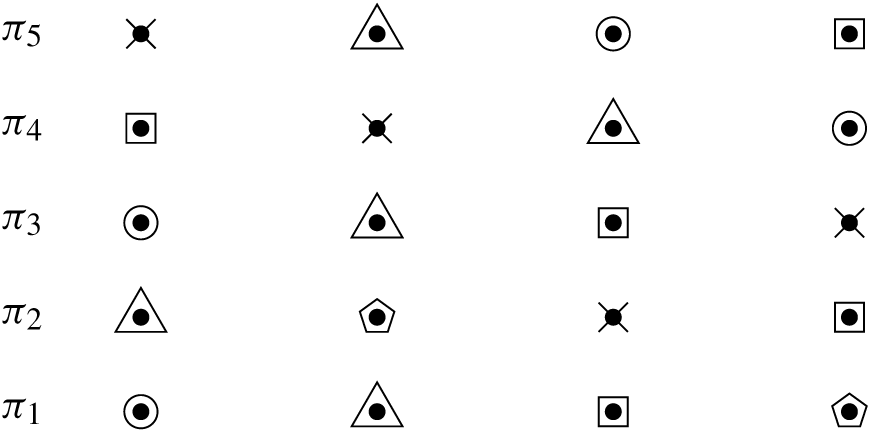
Here, a partition $\rho \in \Pi [n \times r]$ is said to be non-flat if the partition diagram $\Gamma (\pi , \rho )$ of $\rho$ and the partition $\pi$ is non-flat, where $\pi \,:\!= (\pi_1,\ldots , \pi_n) \in \Pi [n\times r]$ with $\pi_k \,:\!= \{ (k,1), \ldots , (k,r) \}$ , $k=1,\ldots , n$ . Figure 1 shows an example of a non-flat partition with $n=5$ , $r=4$ , and

\begin{align} & \triangle = \{ (1,2), (2,1) ,(2,2),(3,3),(4,2)\}, \\ & \ocircle= \{ (1,1), (3,1) ,(4,4),(5,3)\}, \\ & \Box = \{ (1,3), (2,4) ,(3,3),(4,1),(5,4)\}, \\ & \pentagon = \{ (1,4), (2,2)\}, \\ & \times = \{ (2,3), (3,4) ,(4,2),(5,1)\} \\ & \pi_k = \{ (k,1), (k,2) ,(k,3),(k,4),(k,5)\}, \qquad k=1,2,3,4,5. \end{align}

Figure 1.

Example of a non-flat partition.

2.2. Processes vanishing on diagonals

The next consequence of Proposition 2 shows that when $u(z_1,\ldots , z_r;\,\omega )$ vanishes on the diagonals in $X^r$ , the moments of

\begin{equation*} \int_{X^r} u(z_1,\ldots , z_r;\,\omega ) \omega ({\rm d}z_1) \cdots \omega ({\rm d}z_r) \end{equation*}

reduce to sums over non-flat partition diagrams.

Proposition 3. Assume that $u(z_1,\ldots , z_r;\,\omega )=0$ whenever $z_i=z_j$ , $1\leq i\not= j \leq r$ , $\omega \in \Omega^X$ . Then we have

\begin{equation} \nonumber \mathrm{E} \Big[ \Big( \int_{X^r} \hskip-0.2cm u(z_1,\ldots , z_r;\,\omega ) \omega ({\rm d}z_1) \cdots \omega ({\rm d}z_r) \Big)^n \Big] = \hskip-0.3cm \sum_{ \substack{ \rho \in \Pi [n\times r] \\ \rho \wedge \pi = \hat{0} }} \hskip-0.2cm \mathrm{E} \bigg[ \int_{X^{|\rho |}} \hskip-0.2cm \epsilon^+_{\mathfrak{z}_{|\rho |}} \prod_{k=1}^n u ( z^\rho_{\pi_k} ) \hat{\lambda}^{|\rho |} ( {\rm d} \mathfrak{z}_{|\rho |} ) \bigg]. \end{equation}

Proof. Assume that $u(z_1,\ldots , z_r;\,\omega )$ vanishes on diagonals, and let $\rho \in \Pi [n]$ . Then, for any $z_1,\ldots , z_r\in X$ we have

\begin{equation*} \prod_{k=1}^n u( z^\rho_{\pi_k} ) = \prod_{k=1}^n u(z_{\zeta^\rho (k,1)}, \ldots , z_{\zeta^\rho (k,r)} ) = 0 \end{equation*}

whenever $p\,:\!=\zeta^\rho (k,a) = \zeta^\rho (k,b)$ for some $k\in \{1,\ldots , n \}$ and $a\not=b \in \{1,\ldots , r\}$ . According to (5) this implies that ${(k,a)\in \rho_p}$ and ${(k,b)\in \rho_p}$ ; therefore $\rho$ is not a non-flat partition, and it should be excluded from the sum over $\Pi [n]$ .

When $n=1$ , the first moment in Proposition 3 yields the Georgii–Nguyen–Zessin identity

(7) \begin{align} \nonumber \mathrm{E} \Big[ \int_{X^r} u(z_1,\ldots , z_r;\,\omega ) \omega ({\rm d}z_1) \cdots \omega ({\rm d}z_r) \Big] & = \sum_{ \substack{ \rho \in \Pi [1\times r] \\ \rho \wedge \pi = \hat{0} }} \mathrm{E} \Big[ \int_{X^{|\rho |}} \epsilon^+_{\mathfrak{z}_{|\rho |}} u ( z^\rho_{\pi_1} ) \hat{\lambda}^{|\rho |} ( {\rm d} \mathfrak{z}_{|\rho |} ) \Big] \\ & = \mathrm{E} \Big[ \int_{X^r} \epsilon^+_{\mathfrak{z}_r} u(z_1,\ldots ,z_r ;\,\omega ) \hat{\lambda}^r ( {\rm d} \mathfrak{z}_r ) \Big] ; \label{eqn7}\end{align}

see [Reference Kartun-Giles, Kim and Commun9, Lemma IV.1] and [Reference Bogdan, Rosiński, Serafin and Wojciechowski2, Lemma 2.1] for different versions based on the Poisson point process. In the case of second moments, we find that

\begin{multline*} \mathrm{E} \Big[ \Big( \int_{X^r} u(z_1,\ldots , z_r;\,\omega ) \omega ({\rm d}z_1) \cdots \omega ({\rm d}z_r) \Big)^2 \Big] \\ = \sum_{ \substack{ \rho \in \Pi [2\times r] \\ \rho \wedge \pi = \hat{0} }} \mathrm{E} \Big[ \int_{X^{|\rho |}} \epsilon^+_{\mathfrak{z}_{|\rho |}} u ( z^\rho_{\pi_1} ) u ( z^\rho_{\pi_2} ) \hat{\lambda}^{|\rho |} ( {\rm d} \mathfrak{z}_{|\rho |} ) \Big] , \end{multline*}

and since the non-flat partitions in $\Pi [ 2\times r]$ are made of pairs and singletons, this identity can be rewritten as the following consequence of Proposition 3, in which for simplicity of notation we write $\pi_1 = \{1,\ldots ,r\}$ and $\pi_2 = \{r+1,\ldots ,2r\}$ .

Corollary 1. Assume that $u(z_1,\ldots , z_r;\,\omega )=0$ whenever $z_i=z_j$ , $1\leq i\not= j \leq r$ , $\omega \in \Omega^X$ . Then the second moment of the integral of k-processes is given by

\begin{multline*} \mathrm{E} \Big[ \Big( \int_{X^r} u(z_1,\ldots , z_r;\,\omega ) \omega ({\rm d}z_1) \cdots \omega ({\rm d}z_r) \Big)^2 \Big] = \sum_{ A \subset \pi_1 } \frac{1}{(r-|A|)!} \\ \times \hskip-0.3cm \sum_{ \gamma : \pi_2 \to A \cup \{ r+1,\ldots , 2r-|A|\} } \hskip-0.3cm \mathrm{E} \Big[ \int_{X^{2r-|A|}} \hskip-0.1cm \epsilon^+_{\mathfrak{z}_{2r-|A|}} u ( z_{\pi_1} ) u ( z_{\gamma (r+1)} , \ldots , z_{\gamma (2r)} ) \hat{\lambda}^{2r-|A|} ( {\rm d} \mathfrak{z}_{2r-|A|} ) \Big], \end{multline*}

where the above sum is over all bijections $\gamma \,:\, \pi_2 \to A \cup \{ r+1,\ldots , 2r-|A|\}$ .

Proof. We express the partitions $\rho \in \Pi [n\times r]$ with non-flat diagrams $\Gamma ( \pi , \rho )$ in Proposition 4 as the collections of pairs and singletons,

\begin{equation*} \rho = \{ i,\gamma (i) \}\}_{i\in A} \cup \{\{i\}\}_{i \in \pi_1, i\notin A} \cup \{\{i\}\}_{i \in \pi_2, i\notin \gamma (A)}, \end{equation*}

for all subsets $A\subset \pi_1 = \{1,\ldots , r \}$ and bijections $\gamma \,:\, \pi_2 \to A \cup \{ r+1,\ldots , 2r-|A|\}$ .

In the case of 2-processes, Corollary 1 shows that

\begin{eqnarray} \nonumber{ \mathrm{E} \Big[ \Big( \int_{X^2} u(z_1 , z_2;\,\omega ) \omega ({\rm d}z_1) \omega ({\rm d}z_2) \Big)^2 \Big] } \\ \nonumber & = & \sum_{ \substack{ \rho \in \Pi [n\times 2] \\ \rho \wedge \pi = \hat{0} }} \mathrm{E} \Big[ \int_{X^{|\rho |}} \epsilon^+_{\mathfrak{z}_{|\rho |}} \prod_{k=1}^n u( z_{\zeta^\rho (k,1)},z_{\zeta^\rho (k,2)} ) \hat{\lambda}^{|\rho |} ( {\rm d} \mathfrak{z}_{|\rho |} ) \Big] \\ \nonumber & = & \hskip-0.6cm \sum_{ \substack{ A \subset \pi_1 \\ \gamma : \{ 3,4 \} \to A \cup \{ 3,\ldots , 4-|A|\}} } \hskip-0.6cm \frac{1}{(r-|A|)!} \mathrm{E} \Big[ \int_{X^{4-|A|}} \epsilon^+_{\mathfrak{z}_{4-|A|}} u ( z_1, z_2 ) u ( z_{\gamma (3)} , z_{\gamma (4)} ) \hat{\lambda}^{4-|A|} ( {\rm d} \mathfrak{z}_{4-|A|} ) \Big] \\ \nonumber & = & \mathrm{E} \Big[ \int_{X^4} \epsilon^+_{\mathfrak{z}_4} ( u(z_1,z_2 ) u(z_3,z_4 ) ) \hat{\lambda}^4 ( {\rm d} \mathfrak{z}_4 ) \Big] \\ \nonumber & & +\ \mathrm{E} \Big[ \int_{X^3} \epsilon^+_{\mathfrak{z}_3} ( u(z_1,z_2 ) u(z_1,z_3 ) ) \hat{\lambda}^3 ( {\rm d} \mathfrak{z}_3 ) \Big] + \mathrm{E} \Big[ \int_{X^3} \epsilon^+_{\mathfrak{z}_3} ( u(z_2,z_1 ) u(z_3,z_1 ) ) \hat{\lambda}^3 ( {\rm d} \mathfrak{z}_3 ) \Big] \\ \nonumber & & +\ \mathrm{E} \Big[ \int_{X^3} \epsilon^+_{\mathfrak{z}_3} ( u(z_1,z_2 ) u(z_2,z_3 ) ) \hat{\lambda}^3 ( {\rm d} \mathfrak{z}_3 ) \Big] + \mathrm{E} \Big[ \int_{X^3} \epsilon^+_{\mathfrak{z}_3} ( u(z_2,z_1 ) u(z_3,z_2 ) ) \hat{\lambda}^3 ( {\rm d} \mathfrak{z}_3 ) \Big] \\ \nonumber & & +\ \mathrm{E} \Big[ \int_{X^2} \epsilon^+_{\mathfrak{z}_2} ( u(z_1,z_2 ) u(z_1,z_2 ) ) \hat{\lambda}^2 ( {\rm d} \mathfrak{z}_2 ) \Big] + \mathrm{E} \Big[ \int_{X^2} \epsilon^+_{\mathfrak{z}_2} ( u(z_1,z_2 ) u(z_2,z_1 ) ) \hat{\lambda}^2 ( {\rm d} \mathfrak{z}_2 ) \Big] . \end{eqnarray}

Similarly, in the case of 3-processes we find

\begin{align} \nonumber & \mathrm{E} \Big[ \Big( \int_{X^3} u(z_1,z_2, z_3;\,\omega ) \omega ({\rm d}z_1) \omega ({\rm d}z_2) \omega ({\rm d}z_3) \Big)^2 \Big] \\ \nonumber & = \sum_{ \substack{ A \subset \{1,2,3\} \\ \gamma : \{4,5,6\} \to A \cup \{ 4,\ldots , 6-|A|\}} } \frac{1}{(3-|A|)!} \mathrm{E} \Big[ \int_{X^5} \epsilon^+_{\epsilon^+_{\mathfrak{z}_5} } u ( z_1,z_2,z_3 ) u ( z_{\gamma (4)} , z_{\gamma (5)} ,z_{\gamma (6)} ) \hat{\lambda}^5 ( {\rm d} \mathfrak{z}_5 ) \Big] \nonumber\\\ & = \mathrm{E} \Big[ \int_{X^6} \epsilon^+_{\mathfrak{z}_6} u(z_1,z_2,z_3 ) u(z_4,z_5,z_6 ) \hat{\lambda}^{6} ( {\rm d} \mathfrak{z}_6 ) \Big] \nonumber\\ & \quad +\ \frac{1}{2} \sum_{ \gamma : \{4,5,6\} \to \{ 1,5 , 6\} } \mathrm{E} \Big[ \int_{X^5} \epsilon^+_{\mathfrak{z}_5} u ( z_1,z_2,z_3) u ( z_{\gamma (4)} , z_{\gamma (5)} ,z_{\gamma (6)} ) \hat{\lambda}^5 ( {\rm d} \mathfrak{z}_5 ) \Big] \nonumber\\ & \quad +\ \frac{1}{2} \sum_{ \gamma : \{4,5,6\} \to \{ 2,5 , 6\} } \mathrm{E} \Big[ \int_{X^5} \epsilon^+_{\mathfrak{z}_5} u ( z_1,z_2,z_3) u ( z_{\gamma (4)} , z_{\gamma (5)} ,z_{\gamma (6)} ) \hat{\lambda}^5 ( {\rm d} \mathfrak{z}_5 ) \Big] \nonumber\\ & \quad +\ \frac{1}{2} \sum_{ \gamma : \{4,5,6\} \to \{ 3,5 , 6\} } \mathrm{E} \Big[ \int_{X^5} \epsilon^+_{\mathfrak{z}_5} u ( z_1,z_2,z_3) u ( z_{\gamma (4)} , z_{\gamma (5)} ,z_{\gamma (6)} ) \hat{\lambda}^5 ( {\rm d} \mathfrak{z}_5 ) \Big] \nonumber\\ & \quad +\ \phantom{\frac{1}{2}} \sum_{ \gamma : \{4,5,6\} \to \{1,2, 6\} } \mathrm{E} \Big[ \int_{X^4} \epsilon^+_{\mathfrak{z}_4} u ( z_1,z_2,z_3 ) u ( z_{\gamma (4)} , z_{\gamma (5)} ,z_{\gamma (6)} ) \hat{\lambda}^4 ( {\rm d} \mathfrak{z}_4 ) \Big] \nonumber\\ & \quad +\ \phantom{\frac{1}{2}} \sum_{ \gamma : \{4,5,6\} \to \{1,3, 6\} } \mathrm{E} \Big[ \int_{X^4} \epsilon^+_{\mathfrak{z}_4} u ( z_1,z_2,z_3 ) u ( z_{\gamma (4)} , z_{\gamma (5)} ,z_{\gamma (6)} ) \hat{\lambda}^4 ( {\rm d} \mathfrak{z}_4 ) \Big] \nonumber\\ & \quad +\ \phantom{\frac{1}{2}} \sum_{ \gamma : \{4,5,6\} \to \{2,3, 6\} } \mathrm{E} \Big[ \int_{X^4} \epsilon^+_{\mathfrak{z}_4} u ( z_1,z_2,z_3 ) u ( z_{\gamma (4)} , z_{\gamma (5)} ,z_{\gamma (6)} ) \hat{\lambda}^4 ( {\rm d} \mathfrak{z}_4 ) \Big] \nonumber\\ & \quad +\ \phantom{\frac{1}{2}} \sum_{ \gamma : \{4,5,6\} \to \{1,2,3 \} } \mathrm{E} \Big[ \int_{X^3} \epsilon^+_{\mathfrak{z}_3}z u ( z_1,z_2,z_3 ) u ( z_{\gamma (4)} , z_{\gamma (5)} ,z_{\gamma (6)} ) \hat{\lambda}^3 ( {\rm d} \mathfrak{z}_3 ) \Big] . \end{align}

3. Random-connection model

Two point process vertices $x\not= y$ are independently connected in the random-connection graph with the probability H(x,y) given $\omega \in \Omega^X$ , where $H\,:\,X\times X \longrightarrow [0,1]$ . In particular, the 1-hop count ${\bf 1}_{\{ x \leftrightarrow y \} }$ is a Bernoulli random variable with parameter H(x,y), and we have the relation

\begin{equation*} \mathrm{E} \bigg[ \epsilon^+_{\mathfrak{z}_r} \prod_{i=0}^r {\bf 1}_{\{ z_i \leftrightarrow z_{i+1} \} } ( \omega ) \, \Big| \, \omega \bigg] = \prod_{i=0}^r H( z_i , z_{i+1} ) \end{equation*}

for any subset $\{z_0,\ldots , z_{r+1}\}$ of distinct elements of X, where $\mathfrak{z}_r = \{z_1,\ldots , z_r\}$ and $x \leftrightarrow y$ means that $x\in X$ is connected to $y\in X$ .

Given $x,y \in X$ , the number of $(r+1)$ -hop sequences $z_1,\ldots , z_r\in \omega$ of vertices connecting x to y in the random graph is given by the multiparameter stochastic integral

\begin{equation*} N^{x,y}_{r+1} = \int_{X^r} u(z_1,\ldots , z_r ;\,\omega ) \omega ({\rm d}z_1) \cdots \omega ({\rm d}z_r) \end{equation*}

of the $\{0,1\}$ -valued r-process

(8) \begin{equation} u(z_1,\ldots , z_r;\,\omega ) \,:\!= {\bf 1}_{\{ z_i \not= z_j, \, 1\leq i<j \leq r \} } {\bf 1}_{\{ z_1,\ldots , z_r \in \omega \} } \prod_{i=0}^r {\bf 1}_{\{ z_i \leftrightarrow z_{i+1} \} } ( \omega ), \qquad z_1,\ldots , z_r \in X, \label{eqn8} \end{equation}

which vanishes on the diagonals in $X^r$ , with $z_0\,:\!=x$ and $z_{r+1} \,:\!= y$ . In addition, for any distinct $z_1,\ldots , z_r \in X$ and $u(z_1,\ldots , z_r;\,\omega )$ given by (8) we have

(9) \begin{equation} \mathrm{E} [ \epsilon^+_{\mathfrak{z}_r} u(z_1,\ldots , z_r;\,\omega ) \!\mid\! \omega ] = \mathrm{E} \bigg[ \epsilon^+_{\mathfrak{z}_r} \prod_{i=0}^r {\bf 1}_{\{ z_i \leftrightarrow z_{i+1} \} } ( \omega ) \, \Big| \, \omega \bigg] = \prod_{i=0}^r H( z_i , z_{i+1} ), \label{eqn9} \end{equation}

and therefore the first-order moment of the $(r+1)$ -hop count between $x\in X$ and $y\in X$ is given as

(10) \begin{equation} \mathrm{E} \Big[ \int_{X^r} u(z_1,\ldots , z_r;\, \omega ) \omega ({\rm d}z_1) \cdots \omega ({\rm d}z_r) \Big] = \mathrm{E} \bigg[ \int_{X^r} \prod_{i=0}^r H ( z_i , z_{i+1} ) \hat{\lambda}^r ( {\rm d} \mathfrak{z}_r ) \bigg] \label{eqn10} \end{equation}

(see also [Reference Kartun-Giles, Kim and Commun9, Theorem II.1]) as a consequence of the Georgii–Nguyen–Zessin identity (Reference Deng, Zhou, Haenggi and Commun7).

In the next proposition we compute the moments of all orders of r-hop counts as sums over non-flat partition diagrams. The role of the powers $1/n^\rho_{l,i}$ in (Reference Kong, Flint, Wang, Niyato and Privault10) is to ensure that all powers of H(x,y) in (Reference Kong, Flint, Wang, Niyato and Privault10) are equal to one, since all powers of ${\bf 1}_{\{ z \leftrightarrow z' \} }$ in (Reference Mecke11) below are equal to ${\bf 1}_{\{ z \leftrightarrow z' \} }$ .

Proposition 4. The moment of order n of the $(r+1)$ -hop count between $x\in X$ and $y\in X$ is given by

(11) \begin{equation} \mathrm{E} [ ( N^{x,y}_{r+1} )^n ] = \sum_{ \substack{ \rho \in \Pi [n\times r] \\ \rho \wedge \pi = \hat{0} }} \mathrm{E} \bigg[ \int_{X^{|\rho |}} \prod_{l=1}^n \prod_{i=0}^r H^{1/n^\rho_{l,i}}( z_{\zeta^\rho (l,i)} , z_{\zeta^\rho (l,i+1)} ) \hat{\lambda}^{|\rho |} ( {\rm d} \mathfrak{z}_{|\rho|} ) \bigg] , \label{eqn11} \end{equation}

where $z_0=x$ , $z_{r+1}=y$ , $\zeta^\rho (l,0)=0$ , $\zeta^\rho (l,r+1)=r+1$ , and

\begin{equation*} n^\rho_{l,i} = \# \{ (p,j)\in \{1,\ldots ,n\}\times \{0,\ldots , r\} \,:\, \{ \zeta^\rho (l,i) , \zeta^\rho (l,i+1) \} = \{ \zeta^\rho (p,j) , \zeta^\rho (p,j+1) \} \}, \end{equation*}

$1\leq l \leq n$ , $0 \leq i \leq r$ .

Proof. Since $u(z_1,\ldots , z_r;\, \omega )$ vanishes whenever $z_i=z_j$ for some $1\leq i \lt j \leq r$ , by Proposition 3 we have

(12) \begin{eqnarray} \nonumber{ % \! \! \! \! \! \! \! \! \! \! \! \! \! \! \! \! \! \! \! \! \! \! \! \! \! \! \mathrm{E} \bigg[ \bigg( \int_{X^r} u(z_1,\ldots , z_r;\, \omega ) \omega ({\rm d}z_1) \cdots \omega ({\rm d}z_r) \bigg)^n \bigg] } \\ & = & \sum_{ \substack{ \rho \in \Pi [n\times r] \\ \rho \wedge \pi = \hat{0} }} \mathrm{E} \bigg[ \int_{X^{|\rho |}} \prod_{l=1}^n \prod_{i=0}^r {\bf 1}_{\{ z_{\zeta^\rho (l,i)} \leftrightarrow z_{\zeta^\rho (l,i+1)} \} } \hat{\lambda}^{|\rho |} ( {\rm d} \mathfrak{z}_{|\rho|} ) \bigg]\label{eqn12}\ & = & \sum_{ \substack{ \rho \in \Pi [n\times r] \\ \rho \wedge \pi = \hat{0} }} \mathrm{E} \bigg[ \int_{X^{|\rho |}} \prod_{l=1}^n \prod_{i=0}^r H^{1/n^\rho_{l,i}}( z_{\zeta^\rho (l,i)}, z_{\zeta^\rho (l,i+1)} ) \hat{\lambda}^{|\rho |} ( {\rm d} \mathfrak{z}_{|\rho|} ) \bigg], \end{eqnarray}

where we applied (9).

As in Corollary 1, we have the following consequence of Proposition 4, which is obtained by expressing the partitions $\rho \in \Pi [n\times r]$ with non-flat diagrams $\Gamma ( \pi , \sigma )$ as a collection of pairs and singletons.

Corollary 2. The second moment of the $(r+1)$ -hop count between $x\in X$ and $y\in X$ is given by

\begin{multline*} \mathrm{E} [ ( N^{x,y}_{r+1} )^2 ] = \sum_{ \substack{ A \subset \pi_1 \\ \gamma : \{1,\ldots , r\} \to A \cup \{ r+1,\ldots , 2r-|A|\}} } \frac{1}{(r-|A|)!} \\ \times \mathrm{E} \bigg[ \int_{X^{2r-|A|}} \prod_{i=0}^r H^{1/n^\gamma_{1,i}}( z_i , z_{i+1} ) \prod_{j=0}^r H^{1/n^\gamma_{2,j}}( z_{\gamma (j)} , z_{\gamma (j+1) } ) \hat{\lambda}^{2r-|A|} ( {\rm d} \mathfrak{z}_{2r-|A|} ) \bigg], \end{multline*}

where the above sum is over all bijections $\gamma \,:\, \{1,\ldots , r\} \to A \cup \{ r+1,\ldots , 2r-|A|\}$ with $\gamma (0)\,:\!=0$ , $\gamma (r+1)=\!:\,r+1$ , $z_0=\!:\,x$ , and $z_{r+1}\,:\!=y$ , and

\begin{align} n^\gamma_{1,i} = \# \{ j\in \{0,\ldots , r\} \,:\, \{ i , i+1 \} = \{ \gamma ( j) , \gamma (j+1) \} \},\\[3pt] n^\gamma_{2,j} = \# \{ i\in \{0,\ldots , r\} \,:\, ( i , i+1 ) = ( \gamma ( j) , \gamma (j+1) ) \}, \end{align}

for $0 \leq i \leq r$ .

3.1. Variance of 3-hop counts

When $n=2$ and $r=2$ , Corollary 2 allows us to express the variance of the 3-hop count between $x\in X$ and $y\in X$ as follows:

\begin{align} \nonumber & {{\mathrm{{\rm Var}}}} [ N^{x,y}_3 ] \\ \nonumber & = \sum_{ \substack{ \emptyset \not= A \subset \{1,2\} \\ \gamma : \{1,2\} \to A \cup \{ 3 , 4-|A|\}} } \frac{1}{(2-|A|)!} \\ \nonumber & \quad \times \mathrm{E} \bigg[ \int_{X^{4-|A|}} \prod_{i=0}^2 H^{1/n^\gamma_{1,i}}( z_i , z_{i+1} ) \prod_{j=0}^2 H^{1/n^\gamma_{2,j}}( z_{\gamma (j)} , z_{\gamma (j+1) } ) \hat{\lambda}^{4-|A|} ( {\rm d} \mathfrak{z}_{4-|A|} ) \bigg] \\ \nonumber & = \sum_{ \gamma : \{1,2\} \to \{ 1, 4\} } \mathrm{E} \bigg[ \int_{X^3} \prod_{i=0}^2 H^{1/n^\gamma_{1,i}}( z_i , z_{i+1} ) \prod_{j=0}^2 H^{1/n^\gamma_{2,j}}( z_{\gamma (j)} , z_{\gamma (j+1) } ) \hat{\lambda}^3 ( {\rm d} z_1,{\rm d}z_2,{\rm d}z_4 ) \bigg] \\ \nonumber & \quad + \sum_{ \gamma : \{1,2\} \to \{ 2, 4\} }\!\!\!\!\! \mathrm{E} \bigg[ \int_{X^3} \prod_{i=0}^2 H^{1/n^\gamma_{1,i}}( z_i , z_{i+1} ) \prod_{j=0}^2 H^{1/n^\gamma_{2,j}}( z_{\gamma (j)} , z_{\gamma (j+1) } ) \hat{\lambda}^3 ( {\rm d}z_1, {\rm d}z_2, {\rm d}z_4 ) \bigg] \\ \nonumber & \quad + \sum_{ \gamma : \{1,2\} \to \{ 1,2\} }\!\!\!\! \mathrm{E} \bigg[ \int_{X^2} \prod_{i=0}^2 H^{1/n^\gamma_{1,i}}( z_i , z_{i+1} ) \prod_{j=0}^2 H^{1/n^\gamma_{2,j}}( z_{\gamma (j)} , z_{\gamma (j+1) } ) \hat{\lambda}^2 ( {\rm d}z_1,{\rm d}z_2 ) \bigg] . \end{align}

3.2. Variance of 4-hop counts

When $r=3$ and $n=2$ , Corollary 2 yields

\begin{align} {{\mathrm{{\rm Var}}}} [ N^{x,y}_4 ] & = \sum_{ \substack{ \emptyset \not= A \subset \pi_1 \\ \gamma : \{1,\ldots , 3\} \to A \cup \{ 4,\ldots , 6-|A|\}} } \frac{1}{(3-|A|)!} \mathrm{E} \bigg[ \int_{X^{6-|A|}} \prod_{i=0}^3 H^{1/n^\gamma_{1,i}}( z_i , z_{i+1} ) \\ \nonumber & \hskip3cm \qquad \qquad \times \prod_{j=0}^3 H^{1/n^\gamma_{2,j}}( z_{\gamma (j)} , z_{\gamma (j+1) } ) \hat{\lambda}^{6-|A|} ( d \mathfrak{z}_{6-|A|} ) \bigg] \\ \nonumber & = \frac{1}{2} \sum_{ \gamma : \{1,\ldots , 3\} \to \{ 1, 5, 6\} } \mathrm{E} \bigg[ \int_{X^5} \prod_{i=0}^3 H^{1/n^\gamma_{1,i}}( z_i , z_{i+1} ) \\ \nonumber & \hskip3cm \quad \quad \times \prod_{j=0}^3 H^{1/n^\gamma_{2,j}}( z_{\gamma (j)} , z_{\gamma (j+1) } ) \hat{\lambda}^5 ( {\rm d}z_1,{\rm d}z_2,{\rm d}z_3,{\rm d}z_5,{\rm d}z_6 ) \bigg] \\ \nonumber & \quad + \frac{1}{2} \sum_{ \gamma : \{1,\ldots , 3\} \to \{ 2, 5, 6\} } \mathrm{E} \bigg[ \int_{X^5} \prod_{i=0}^3 H^{1/n^\gamma_{1,i}}( z_i , z_{i+1} ) \\ \nonumber & \hskip3cm \quad \quad \times \prod_{j=0}^3 H^{1/n^\gamma_{2,j}}( z_{\gamma (j)} , z_{\gamma (j+1) } ) \hat{\lambda}^5 ( {\rm d}z_1,{\rm d}z_2,{\rm d}z_3,{\rm d}z_5,{\rm d}z_6 ) \bigg] \\ \nonumber & \quad + \frac{1}{2} \sum_{ \gamma : \{1,\ldots , 3\} \to \{ 3, 5, 6\} } \mathrm{E} \bigg[ \int_{X^5} \prod_{i=0}^3 H^{1/n^\gamma_{1,i}}( z_i , z_{i+1} ) \\ \nonumber & \hskip3cm \quad \quad \times \prod_{j=0}^3 H^{1/n^\gamma_{2,j}}( z_{\gamma (j)} , z_{\gamma (j+1) } ) \hat{\lambda}^5 ( {\rm d}z_1,{\rm d}z_2,{\rm d}z_3,{\rm d}z_5,{\rm d}z_6 ) \bigg] \\ \nonumber & \quad + \phantom{\frac{1}{2}} \sum_{ \gamma : \{1,\ldots , 3\} \to \{ 1,2, 6\} } \mathrm{E} \bigg[ \int_{X^4} \prod_{i=0}^3 H^{1/n^\gamma_{1,i}}( z_i , z_{i+1} ) \\ \nonumber & \hskip3cm \quad \quad \times \prod_{j=0}^3 H^{1/n^\gamma_{2,j}}( z_{\gamma (j)} , z_{\gamma (j+1) } ) \hat{\lambda}^4 ( {\rm d}z_1,{\rm d}z_2,{\rm d}z_3,{\rm d}z_6 ) \bigg] \\ \nonumber & \quad + \phantom{\frac{1}{2}} \sum_{ \gamma : \{1,\ldots , 3\} \to \{ 1,3, 6\} } \mathrm{E} \bigg[ \int_{X^4} \prod_{i=0}^3 H^{1/n^\gamma_{1,i}}( z_i , z_{i+1} ) \\ \nonumber & \hskip3cm \quad \quad \times \prod_{j=0}^3 H^{1/n^\gamma_{2,j}}( z_{\gamma (j)} , z_{\gamma (j+1) } ) \hat{\lambda}^4 ( {\rm d}z_1,{\rm d}z_2,{\rm d}z_3,{\rm d}z_6 ) \bigg] \\ \nonumber & \quad + \phantom{\frac{1}{2}} \sum_{ \gamma : \{1,\ldots , 3\} \to \{ 2,3, 6\} } \mathrm{E} \bigg[ \int_{X^4} \prod_{i=0}^3 H^{1/n^\gamma_{1,i}}( z_i , z_{i+1} ) \\ \nonumber & \hskip3cm \quad \quad \times \prod_{j=0}^3 H^{1/n^\gamma_{2,j}}( z_{\gamma (j)} , z_{\gamma (j+1) } ) \hat{\lambda}^4 ( {\rm d}z_1,{\rm d}z_2,{\rm d}z_3,{\rm d}z_6 ) \bigg] \\ \nonumber & \quad + \phantom{\frac{1}{2}} \sum_{ \gamma : \{1,\ldots , 3\} \to \{1,\ldots , 3\} } \mathrm{E} \bigg[ \int_{X^3} \prod_{i=0}^3 H^{1/n^\gamma_{1,i}}( z_i , z_{i+1} ) \\ \nonumber & \hskip3cm \quad \quad \times \prod_{j=0}^3 H^{1/n^\gamma_{2,j}}( z_{\gamma (j)} , z_{\gamma (j+1) } ) \hat{\lambda}^3 ( {\rm d}z_1,{\rm d}z_2,{\rm d}z_3 ) \bigg]. \end{align}

4. Poisson case

In this section and the next one we will work in the Poisson random-connection model, using a Poisson point process on $X={{\mathord{\mathbb R}}}^d$ with intensity $\lambda ({\rm d}x)$ on ${{\mathord{\mathbb R}}}^d$ . We let

(13) \begin{equation} H^{(n)} (x_0,x_n ) \,:\!= \int_{{{\mathord{\mathbb R}}}^d} \cdots \int_{{{\mathord{\mathbb R}}}^d} \prod_{i=0}^{n-1} H (x_i,x_{i+1}) \lambda ({\rm d}x_1) \cdots \lambda ({\rm d}x_{n-1}), \qquad x_0, x_n \in {{\mathord{\mathbb R}}}^d, \ n \geq 1.\quad \label{eqn13} \end{equation}

The 2-hop count between $x\in {{\mathord{\mathbb R}}}^d$ and $y\in {{\mathord{\mathbb R}}}^d$ is given by the first-order stochastic integral

\begin{equation*} \int_{{{\mathord{\mathbb R}}}^d} u(z;\,\omega ) \omega ({\rm d}z) = \int_{{{\mathord{\mathbb R}}}^d} {\bf 1}_{\{ x \leftrightarrow z_1 \} } {\bf 1}_{\{ z_1 \leftrightarrow y \} } ( \omega ) \omega ({\rm d}z_1) = \int_{{{\mathord{\mathbb R}}}^d} {\bf 1}_{\{ x \leftrightarrow z_1 \} } {\bf 1}_{\{ z_1 \leftrightarrow y \} } \omega ({\rm d}z_1), \end{equation*}

and its moment of order n is

\begin{align} \mathrm{E} \bigg[ \bigg( \int_{{{\mathord{\mathbb R}}}^d} u(z_1;\,\omega ) \omega ({\rm d}z_1) \bigg)^n \bigg] & = \mathrm{E} \bigg[ \bigg( \int_{{{\mathord{\mathbb R}}}^d} {\bf 1}_{\{ x \leftrightarrow z_1 \} } {\bf 1}_{\{ z_1 \leftrightarrow y \} } \omega ({\rm d}z_1) \bigg)^n \bigg] \\ & = \sum_{ \substack{ \rho \in \Pi [n\times 1] }} \int_{X^{|\rho |}} \prod_{l=1}^{|\rho |} \big( H(x,z_l)H(z_l,y) \big) \lambda^{|\rho |} ( {\rm d}z_1,\ldots , {\rm d}z_{|\rho|} ) \\ & = \sum_{k=1}^n S(n,k) \bigg( \int_{{{\mathord{\mathbb R}}}^d} H(x,z)H(z,y) \lambda ( {\rm d} z ) \bigg)^k \\ & = \sum_{k=1}^n S(n,k) \big( H^{(2)} (x,y) \big)^k ; \end{align}

therefore, from (3), the 2-hop count between $x\in {{\mathord{\mathbb R}}}^d$ and $y\in {{\mathord{\mathbb R}}}^d$ is a Poisson random variable with mean

\begin{equation*} H^{(2)}(x,y) = \int_{{{\mathord{\mathbb R}}}^d} H(x,z)H(z,y) \lambda ( {\rm d} z ). \end{equation*}

By (10), the first-order moment of the r-hop count is given by

\begin{equation*} H^{(r)}(x,y) = \int_{X^{r-1}} \prod_{i=0}^{r-1} H ( z_i , z_{i+1} ) \lambda^{r-1} ( {\rm d}z_1, \ldots {\rm d}z_{r-1} ). \end{equation*}

Corollary 3. The variance of the r-hop count between $x\in {{\mathord{\mathbb R}}}^d$ and $y\in {{\mathord{\mathbb R}}}^d$ is given by

\begin{align} \nonumber {{\mathrm{{\rm Var}}}} [ N^{x,y}_r ] & = \sum_{p=1}^{r-1} \sum_{ \substack{ 1\leq k_1 \lt\cdots \lt k_p \lt r \\ 1 \leq l_1 \lt\cdots \lt l_p \lt r } }\, \sum_{\sigma \in \Sigma [p]} \int_{X^p} \prod_{ 0 \leq i \leq p } H^{(k_{i+1}-k_i)}( z_i , z_{i+1} ) \hskip-0.8cm \\ \nonumber & \quad \times \prod_{ \substack{ 0 \leq j \leq p \\ l_{\sigma (j+1)}-l_{\sigma (j)} + k_{j+1}-k_j > 2 \\ \mbox{\scriptsize or } \{j,j+1\} \not= \{ \sigma (j), \sigma (j+1) \}} } \hskip-0.8cm H^{(l_{\sigma (j+1)}-l_{\sigma (j)})}( z_{\sigma (j)} , z_{\sigma ( j+1 ) } ) \lambda^p ( {\rm d} \mathfrak{z}_p ), \end{align}

with $k_0=l_0=0$ , $k_{p+1}=l_{p+1}=r$ , $\sigma (0)=0$ , and $\sigma (r)=r$ , where the above sum is over all permutations $\sigma \in \Sigma [p]$ of $\{1,\ldots , p\}$ .

Proof. We rewrite the result of Corollary 2 by denoting the set $A\subset \pi_1$ as $A = \{k_1, \ldots , k_p \}$ , for $1\leq k_1 \lt\cdots \lt k_p \leq r-1$ , and we identify $\gamma (A) \subset A \cup \{ r+1,\ldots , 2r-|A|\}$ with $\{l_1, \ldots , l_p \}$ , which requires a sum over the permutations of $\{1,\ldots , p\}$ since $1\leq l_1 \lt\cdots \lt l_p \leq r-1$ , where $1 \leq p \leq r-1$ . In addition, the multiple integrals over contiguous index sets in $A^c$ are evaluated using (Reference Miyoshi and Shirai13).

4.1. Variance of 3-hop counts

When $n=2$ and $r=2$ Corollary 3 allows us to compute the variance of the 3-hop count between $x\in {{\mathord{\mathbb R}}}^d$ and $y\in {{\mathord{\mathbb R}}}^d$ , as follows:

(14) \begin{multline} {{\mathrm{{\rm Var}}}} [ N^{x,y}_3 ] = 2 \int_{{{\mathord{\mathbb R}}}^d} H(x,z_1)H^{(2)}(z_1,y) H^{(2)}(z_1,y)\\ + 2 \int_{{{\mathord{\mathbb R}}}^d}\\ H(x,z_1)H^{(2)}(x,z_1)H^{(2)}(z_1,y)H(z_1,y) \lambda ( {\rm d} z_1 ) + \int_{X^2} H(x,z_1)H(z_1,z_2)H(z_2,y) H(x,z_2) H(z_1,y) \lambda^2 ( {\rm d} z_1,{\rm d}z_2 ) + H^{(3)}(x,y) . \label{eqn16}\end{multline}

By Corollary 3 the variance of 4-hop counts can be similarly computed explicitly as a sum of 33 terms.

5. Rayleigh fading

In this section we consider a Poisson point process on $X={{\mathord{\mathbb R}}}^d$ with flat intensity $\lambda ({\rm d}x) = \lambda {\rm d}x$ on ${{\mathord{\mathbb R}}}^d$ , $\lambda \gt0$ , and a Rayleigh fading function of the form

\begin{equation*} H_\beta ( x , y ) \,:\!= \rm{e}^{- \beta \Vert x - y \Vert^2 }, \qquad x, y \in {{\mathord{\mathbb R}}}^d, \ \beta \gt0. \end{equation*}

Lemmas 1 and 2 can be used to evaluate the integrals appearing in Corollary 3 and in the variance (Reference Nguyen and Zessin14) of the 3-hop counts.

Lemma 1. For all $n\geq 1$ , $y_1,\ldots, y_n \in {{\mathord{\mathbb R}}}^d$ , and $\beta_1, \ldots , \beta_n \gt0$ we have

\begin{align} & \int_{{{\mathord{\mathbb R}}}^d} \prod_{i=1}^n H_{\beta_i} (x,y_i) {\rm d}x \\ & \qquad = \bigg( \frac{\pi }{\beta_1+\cdots + \beta_n}\bigg)^{d/2} \, \prod_{i=1}^{n-1} H_{\frac{\beta_{i+1} (\beta_1+\cdots + \beta_i)}{\beta_1+\cdots + \beta_{i+1}}} \bigg( y_{i+1}, \frac{\beta_1 y_1+ \cdots + \beta_i y_i}{\beta_1+\cdots +\beta_i } \bigg) . \end{align}

Proof. We start by showing that for all $n\geq 1$ we have

(15) \begin{multline} \prod_{i=1}^n H_{\beta_i} (x,y_i)\\ & = H_{\beta_1+\cdots + \beta_n} \bigg(x,\frac{\beta_1 y_1+ \cdots + \beta_n y_n}{\beta_1+\cdots +\beta_n }\bigg) \,\prod_{i=1}^{n-1} H_{\frac{\beta_{i+1}(\beta_1+\cdots + \beta_i)}{\beta_1+\cdots + \beta_{i+1} }} \bigg( y_{i+1}, \frac{\beta_1 y_1+ \cdots + \beta_i y_i}{\beta_1+\cdots +\beta_i } \bigg). \label{eqn18}\end{multline}

Clearly, this relation holds for $n=1$ . In addition, at the rank $n=2$ we have

\begin{eqnarray} { H_{\beta_1} (x,y_1)H_{\beta_2} (x,y_2) = \rm{e}^{-\beta_1 \Vert y_1-x\Vert^2 } \rm{e}^{-\beta_2 \Vert x -y_2\Vert^2 } } \\ & = & %\rm{e}^ \exp\{-\beta_1 \Vert y_1\Vert^2 -\beta_2 \Vert y_2\Vert^2 + 2 \langle \beta_1y_1 + \beta_2 y_2, x\rangle - ( \beta_1 + \beta_2 ) \Vert x\Vert^2 \} \\ & = & %\rm{e}^ \exp\{-\beta_1 \Vert y_1\Vert^2 -\beta_2 \Vert y_2\Vert^2 - ( \beta_1 + \beta_2 ) \Vert x - ( \beta_1y_1 + \beta_2 y_2)/(\beta_1+\beta_2 ) \Vert^2 \\ &&\qquad + \Vert \beta_1y_1 + \beta_2 y_2 \Vert^2/(\beta_1+\beta_2 ) \} \\ & = & %\rm{e}^ \exp\{- ( \beta_1 + \beta_2 ) \Vert x - ( \beta_1y_1 + \beta_2 y_2)/(\beta_1+\beta_2 ) \Vert^2 - \beta_1 \beta_2 \Vert y_1-y_2\Vert^2 /(\beta_1+\beta_2 ) \} \\ & = & H_{\beta_1+\beta_2} \bigg(x , \frac{\beta_1y_1 + \beta_2 y_2}{\beta_1+\beta_2} \bigg) H_{\frac{ \beta_1 \beta_2 }{\beta_1+\beta_2 }}(y_1,y_2). % , \end{eqnarray}

Next, assuming that (15) holds at the rank $n\geq 1$ , we have

\begin{eqnarray} { \prod_{i=1}^{n+1} H_{\beta_i} (x,y_i) = H_{\beta_{n+1}} (x,y_{n+1}) H_{\beta_1+\cdots + \beta_n} \bigg(x,\frac{\beta_1 y_1+ \cdots + \beta_n y_n}{\beta_1+\cdots +\beta_n }\bigg) } \\ & & \times \prod_{i=1}^{n-1} H_{\frac{\beta_{i+1}(\beta_1+\cdots + \beta_i)}{\beta_1+\cdots + \beta_{i+1}}} \bigg( y_{i+1}, \frac{\beta_1 y_1+ \cdots + \beta_i y_i}{\beta_1+\cdots +\beta_i } \bigg) \\ & = & H_{\beta_1+\cdots + \beta_{n+1}} \bigg(x,\frac{\beta_1 y_1+ \cdots + \beta_{n+1} y_{n+1}}{\beta_1+\cdots +\beta_n }\bigg) \\ & & \times \prod_{i=1}^n H_{\frac{\beta_{i+1}(\beta_1+\cdots + \beta_i)}{\beta_1+\cdots + \beta_{i+1}}} \bigg( y_{i+1}, \frac{\beta_1 y_1+ \cdots + \beta_i y_i}{\beta_1+\cdots +\beta_i } \bigg). \end{eqnarray}

As a consequence, we find that

\begin{multline*} \int_{{{\mathord{\mathbb R}}}^d} \prod_{i=1}^n H_{\beta_i} (x,y_i) {\rm d}x = \prod_{i=1}^{n-1} H_{\frac{\beta_{i+1}(\beta_1+\cdots + \beta_i)}{\beta_1+\cdots + \beta_{i+1}}} \bigg( y_{i+1}, \frac{\beta_1 y_1+ \cdots + \beta_i y_i}{\beta_1+\cdots +\beta_i } \bigg) \\ \hskip2.5cm \times \int_{{{\mathord{\mathbb R}}}^d} H_{\beta_1+\cdots + \beta_n} \bigg(x,\frac{\beta_1 y_1+ \cdots + \beta_n y_n}{\beta_1+\cdots +\beta_n }\bigg) {\rm d}x \\ = \bigg( \frac{\pi }{\beta_1+\cdots + \beta_n}\bigg)^{d/2} \prod_{i=1}^{n-1} H_{\frac{\beta_{i+1}(\beta_1+\cdots + \beta_i)}{\beta_1+\cdots + \beta_{i+1}}} \bigg( y_{i+1}, \frac{\beta_1 y_1+ \cdots + \beta_i y_i}{\beta_1+\cdots +\beta_i } \bigg). \end{multline*}

In particular, applying Lemma 1 for $n=2$ yields

(16) \begin{align} \nonumber \int_{{{\mathord{\mathbb R}}}^d} H_{\beta_1} ( y_1,x ) H_{\beta_2} ( x ,y_2 ) {\rm d}x & = \Big( \frac{\pi }{\beta_1 + \beta_2 }\Big)^{d/2} H_{\frac{\beta_1\beta_2}{\beta_1+\beta_2 }} ( y_1,y_2) \\ & = \Big( \frac{\pi }{\beta_1 + \beta_2 }\Big)^{d/2} \rm{e}^{- \beta_1\beta_2 \Vert y_1- y_2\Vert^2/ ( \beta_1+\beta_2 ) }, \quad y_1,y_2 \in {{\mathord{\mathbb R}}}^d, \label{eqn19}\end{align}

and the 2-hop count between $x\in {{\mathord{\mathbb R}}}^d$ and $y\in {{\mathord{\mathbb R}}}^d$ is a Poisson random variable with mean

\begin{eqnarray} \nonumber H^{(2)}_\beta (x,y) & = & \lambda \int_{{{\mathord{\mathbb R}}}^d} H_\beta ( x,z ) H_\beta ( z ,y ) {\rm d}z \\ \nonumber & = & \lambda \Big( \frac{\pi }{2 \beta }\Big)^{d/2} H_{\beta /2} ( x,y) \\ \nonumber & = & \lambda \Big( \frac{\pi }{2 \beta }\Big)^{d/2} \rm{e}^{- \Vert x- y\Vert^2/ 2}. \end{eqnarray}

By an induction argument similar to that of Lemma 1, we obtain the following lemma.

Lemma 2. For all $n \geq 1$ , $x_0,\ldots, x_n \in {{\mathord{\mathbb R}}}^d$ , and $\beta_1, \ldots , \beta_n \gt0$ we have

\begin{multline*} \int_{{{\mathord{\mathbb R}}}^d} \cdots \int_{{{\mathord{\mathbb R}}}^d} \prod_{i=1}^n H_{\beta_i} (x_{i-1},x_i) \,{\rm d} x_1 \cdots {\rm d}x_{n-1} \\ = \bigg( \frac{\pi^{n-1} }{\sum_{i=1}^n \beta_1 \cdots \beta_{i-1}\beta_{i+1}\cdots \beta_n }\bigg)^{d/2} H_{\frac{\beta_1 \cdots \beta_n}{\sum_{i=1}^n \beta_1 \cdots \beta_{i-1}\beta_{i+1}\cdots \beta_n }} (x_0,y_n). \end{multline*}

Proof. Clearly the relation holds at the rank $n=1$ . Assuming that it holds at the rank $n\geq 1$ and using (16), we have

\begin{align} & \int_{{{\mathord{\mathbb R}}}^d} \cdots \int_{{{\mathord{\mathbb R}}}^d} \prod_{i=1}^{n+1} H_{\beta_i} (x_{i-1},x_i) \,{\rm d} x_1 \cdots {\rm d}x_n \\ & = \int_{{{\mathord{\mathbb R}}}^d} H_{\beta_{n+1}} (x_n,x_{n+1}) \int_{{{\mathord{\mathbb R}}}^d} \cdots \int_{{{\mathord{\mathbb R}}}^d} \prod_{i=1}^n H_{\beta_i} (x_{i-1},x_i) \,{\rm d} x_1 \cdots {\rm d}x_n \\ & = \bigg( \frac{\pi^{n-1} }{\sum_{i=1}^n \beta_1 \cdots \beta_{i-1}\beta_{i+1}\cdots \beta_n }\bigg)^{d/2} \\ & \quad \times \int_{{{\mathord{\mathbb R}}}^d} H_{\frac{\beta_1 \cdots \beta_n}{\sum_{i=1}^n \beta_1 \cdots \beta_{i-1}\beta_{i+1}\cdots \beta_n }} (x_0,x_n) H_{\beta_{n+1}} (x_n,x_{n+1}) \,{\rm d} x_n \\ & = \bigg( \frac{\pi^{n-1} }{\sum_{i=1}^n \beta_1 \cdots \beta_{i-1}\beta_{i+1}\cdots \beta_n }\bigg)^{d/2} \\ & \quad \times \bigg( \frac{\pi }{\frac{\beta_1 \cdots \beta_n}{\sum_{i=1}^n \beta_1 \cdots \beta_{i-1}\beta_{i+1}\cdots \beta_n } + \beta_{n+1}}\bigg)^{d/2} H_{\frac{\beta_1 \cdots \beta_{n+1}}{\sum_{i=1}^{n+1} \beta_1 \cdots \beta_{i-1}\beta_{i+1}\cdots \beta_{n+1}}} ( x_0,x_{n+1}). \end{align}

In particular, the first-order moment of the r-hop count between $x_0\in {{\mathord{\mathbb R}}}^d$ and $x_r\in {{\mathord{\mathbb R}}}^d$ is given by

(17) \begin{eqnarray} \nonumber H^{(r)}_\beta (x_0,x_r) & = & \int_{{{\mathord{\mathbb R}}}^d} \cdots \int_{{{\mathord{\mathbb R}}}^d} \prod_{i=0}^{r-1} H_\beta (x_i,x_{i+1}) \lambda ( {\rm d}x_1 ) \cdots \lambda ( {\rm d}x_{r-1} ) \\ \nonumber & = & \lambda^{r-1} \bigg( \frac{\pi^{r-1} }{r \beta^{r-1} }\bigg)^{d/2} H_{\beta / r } (x,y) \\ & = & \lambda^{r-1} \bigg( \frac{\pi^{r-1} }{r \beta^{r-1} }\bigg)^{d/2} \rm{e}^{- \beta \Vert x- y\Vert^2/r}, \qquad x, y \in {{\mathord{\mathbb R}}}^d. \label{eqn20}\end{eqnarray}

5.1. Variance of 3-hop counts

Corollary 3 and Lemma 2 allow us to recover Theorem II.3 of [Reference Kartun-Giles, Kim and Commun9] for the variance of 3-hop counts by a shorter argument, while extending it from the plane $X = {{\mathord{\mathbb R}}}^2$ to $X = {{\mathord{\mathbb R}}}^d$ .

Corollary 4. The variance of the 3-hop count between $x\in {{\mathord{\mathbb R}}}^d$ and $y\in {{\mathord{\mathbb R}}}^d$ is given by

\begin{eqnarray} {{\mathrm{{\rm Var}}}} [ N^{x,y}_3 ] & = & 2 \lambda^3 \Big( \frac{\pi^3}{8 \beta^3} \Big)^{d/2} \rm{e}^{- \beta \Vert x- y\Vert^2/2} + \lambda^2 \Big( \frac{\pi^2 }{3 \beta^2 }\Big)^{d/2} \rm{e}^{- \beta \Vert x- y\Vert^2/3} \\ & & +\ 2 \lambda^3 \Big( \frac{\pi^3}{12 \beta^3} \Big)^{d/2} \rm{e}^{- 3 \beta \Vert x- y\Vert^2/4} + \lambda^2 \Big( \frac{\pi^2}{8 \beta^2 } \Big)^{d/2} \rm{e}^{- \beta \Vert x- y\Vert^2 } . \end{eqnarray}

Proof. By (Reference Privault17) and Lemma 2 we have

\begin{align} & \int_{{{\mathord{\mathbb R}}}^d} H_\beta (x,z_1)H^{(2)}_\beta (z_1,y) H^{(2)}_\beta (z_1,y) \lambda ( {\rm d} z_1 ) \\ & = \lambda^2 \Big( \frac{\pi^2}{4\beta^2} \Big)^{d/2} \int_{{{\mathord{\mathbb R}}}^d} H_\beta (x,z_1)H^2_{\beta /2} (z_1,y) \lambda ( {\rm d} z_1 ) \end{align}

\begin{align} & \quad = \lambda^3 \Big( \frac{\pi^2}{4\beta^2} \Big)^{d/2} \int_{{{\mathord{\mathbb R}}}^d} H_\beta (x,z_1)H_\beta (z_1,y) \lambda ( {\rm d} z_1 ) = \lambda^3 \Big( \frac{\pi^3}{8\beta^3} \Big)^{d/2} H_{\beta /2} (x,y);\\ & \int_{{{\mathord{\mathbb R}}}^d} H_\beta (x,z_1)H^{(2)}_\beta (x,z_1)H^{(2)}_\beta (z_1,y)H_\beta (z_1,y) \lambda ( {\rm d} z_1 ) \\ \nonumber & \quad = \lambda^2 \Big( \frac{\pi^2}{4\beta^2} \Big)^{d/2} \int_{{{\mathord{\mathbb R}}}^d} H_{3\beta/2} (z_1,y) H_{3\beta /2} (x,z_1) \lambda ( {\rm d} z_1 ) = \lambda^3 \Big( \frac{\pi^3}{12\beta^3} \Big)^{d/2} H_{3\beta /4} (x,y) ;\\ & \int_{X^2} H_\beta (x,z_1)H_\beta (z_1,z_2)H_\beta (z_2,y) H_\beta (x,z_2) H_\beta (z_1,y) \lambda^2 ( {\rm d} z_1,{\rm d}z_2 ) \\ & \quad = \lambda \Big( \frac{\pi}{3\beta} \Big)^{d/2} H_\beta (x,y) \int_{{{\mathord{\mathbb R}}}^d} H_{2\beta/3 }(z_2,(x+y)/2) H_{2\beta }(z_2,(x+y)/2) \lambda ( {\rm d} z_2 ) \\ & \quad = \lambda^2 \Big( \frac{\pi^2}{8 \beta^2 } \Big)^{d/2} H_\beta ( x , y ) ; \end{align}

and we conclude by (14).