1 Introduction
Wall-bounded turbulence rarely flows over spatially uniform roughness. Applications abound where roughness, and hence the wall shear stress, varies spatially, with examples including barnacle clusters on ship hulls, rivet rows on aircraft and wind-turbine arrays in wind farms. Loosely speaking, spatially varying roughness is characterised by statistical variations of roughness elements occurring over wall-parallel scales that are comparable or exceed the large scales of wall turbulence. In contrast, spatially uniform roughness is characterised by length scales that are all smaller than the large scales of wall turbulence. Although there currently exist well-established scaling laws that underpin textbook methods such as the Moody chart (Moody Reference Moody1944) for predicting turbulent flows over spatially uniform roughness, the same cannot be said of spatially varying roughness. Predictions for the spatially varying regime can be obtained by extrapolating from the spatially uniform regime but this comes at the cost of uncertainties that are currently not well quantified, with even the delineation between the two regimes currently not well appreciated. The present investigation is an attempt to address these issues as well as to shed light on the general changes to the similarity and structure of rough-wall turbulence from the spatially uniform through to the spatially varying regime. This is achieved by analysing direct numerical simulation (DNS) data of turbulent flow through a channel bounded by walls idealised with laterally varying roughness whereby the scale of roughness variation can be systematically varied while secondary or non-essential parameters are respectively fixed, minimised or eliminated.
1.1 Idealisation of spatially varying roughness
Progress in understanding specific complex turbulent boundary layer flows is often aided by reducing the problem into a set of canonical configurations and drawing general conclusions about a broader class of turbulent flows. In distilling the wider problem of spatially varying roughness, two issues need to be tackled: first is the representation of the roughness and second is the choice of the spatial variation. In the following, we discuss the rationale of our present treatment of these issues.
The first issue is the representation of roughness. As far as the turbulent inertial motions in the log and outer layers are concerned, classical understanding of wall turbulence dictates that the only relevant parameters are the wall shear stress
 $\unicode[STIX]{x1D70F}_{0}$
and the outer scale
 $\unicode[STIX]{x1D6FF}$
, which, for the present flow, is equal to the half-channel height. The turbulent inertial motion disregards whether the wall is smooth or rough and, for a rough wall in particular, the roughness height
 $k$
does not play a direct role even though it sets
 $\unicode[STIX]{x1D70F}_{0}$
. This is of course the outer-layer similarity hypothesis of Townsend (Reference Townsend1976), which is based upon dimensional considerations and backed by evidence overwhelmingly in its favour (Flack & Schultz Reference Flack and Schultz2014). Further, in an idealised simulation in which
 $k$
is entirely eliminated by directly imposing a uniform
 $\unicode[STIX]{x1D70F}_{0}$
as boundary condition, we previously showed that turbulent inertial motions are essentially similar in the log and outer layers (Chung, Monty & Ooi Reference Chung, Monty and Ooi2014). In light of this classical understanding, if the purpose is to study the impact of spatial variations of roughness on turbulent inertial motions, then extending the idealised simulations of Chung et al. (Reference Chung, Monty and Ooi2014) by imposing spatial variations directly on
 $\unicode[STIX]{x1D70F}_{0}$
and circumventing
 $k$
appears to be a sensible approach. Imposing spatial variations directly on
 $\unicode[STIX]{x1D70F}_{0}$
comes at the cost of not knowing how
 $k$
sets
 $\unicode[STIX]{x1D70F}_{0}$
but this issue is perhaps better addressed in research pertaining to spatially uniform roughness, where the preoccupation has been and continues to be the mapping between the geometric parameter
 $k$
to the dynamic parameter
 $k_{s}$
that leads to
 $\unicode[STIX]{x1D70F}_{0}$
for any given roughness (e.g. Raupach, Antonia & Rajagopalan Reference Raupach, Antonia and Rajagopalan1991; Jiménez Reference Jiménez2004; Flack & Schultz Reference Flack and Schultz2014). Imposing spatial variations directly on
 $\unicode[STIX]{x1D70F}_{0}$
comes with the benefit of low blockage by roughness, that is, small
 $k/\unicode[STIX]{x1D6FF}$
. Since the imposed stresses are viscous, the roughness sublayer
 $k$
is replaced by the viscous sublayer
 $10\unicode[STIX]{x1D708}/u_{\unicode[STIX]{x1D70F}}$
, where
 $\unicode[STIX]{x1D708}$
is the kinematic viscosity and
 $u_{\unicode[STIX]{x1D70F}}\equiv (\unicode[STIX]{x1D70F}_{0}/\unicode[STIX]{x1D70C})^{1/2}$
, the friction velocity. As such, the blockage is small but finite,
 $(10\unicode[STIX]{x1D708}/u_{\unicode[STIX]{x1D70F}})/\unicode[STIX]{x1D6FF}=10/\unicode[STIX]{x1D6FF}^{+}$
. The requirement of low blockage, often numerically quoted as
 $k/\unicode[STIX]{x1D6FF}\lesssim 1/40$
(Jiménez Reference Jiménez2004), is necessary in order to distinguish between flow over roughness proper, in which a log layer remains intact and therefore generalisable to other wall-bounded flows, versus flow over obstacles, in which a log layer is absent and therefore specific to a particular outer-flow geometry. The low-blockage requirement is often prohibitively expensive for simulations that resolve roughness elements but the choice of idealisation here ensures that the simulations remain relevant to the roughness regime as opposed to the obstacle regime while being manageable with regards to computational cost, thereby enabling us to perform our intended parametric investigation. The directly imposed variation on
 $\unicode[STIX]{x1D70F}_{0}$
also avoids issues related to changes to the dynamic origin, or step, which typically accompanies a variation in the roughness height.
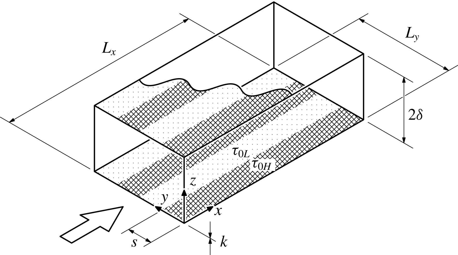
Set-up of idealised DNS to investigate the effect of lateral wall shear stress variations. The width of each uniform-stress patch is
 $s=s_{H}=s_{L}$
. The stress pattern at the top wall (partially shown) is simply the reflection, across the channel centreline, of the bottom wall. The streamwise wall shear stresses are low in dotted regions labelled
 $\unicode[STIX]{x1D70F}_{0L}$
and high in the hatched regions labelled
 $\unicode[STIX]{x1D70F}_{0H}$
.

The second issue is the choice of the spatial variation of roughness (wall shear stress). Spatial variations in roughness can and do occur in any number of ways. A useful classification has been to restrict the variation to occur in only one direction at a time. Within this classification are two configurations that have been the subject of previous research: longitudinally (streamwise-) varying roughness and laterally (spanwise-) varying roughness. We will here focus on laterally varying roughness, and specifically, square-wave variations, that is, patches of laterally alternating otherwise-uniform high or low wall shear stress, respectively
 $\unicode[STIX]{x1D70F}_{0H}$
and
 $\unicode[STIX]{x1D70F}_{0L}$
(figure 1). Apart from being simple, uniform-stress patches are fairly common, arising from man-made or natural boundaries. Two parameters need to be further specified, namely, the wall shear stress ratio
 $\unicode[STIX]{x1D70F}_{0H}/\unicode[STIX]{x1D70F}_{0L}$
, and the lateral size of high and low uniform-stress patches,
 $s_{H}$
and
 $s_{L}$
. Here we fix
 $\unicode[STIX]{x1D70F}_{0H}/\unicode[STIX]{x1D70F}_{0L}=3$
,
 $s_{H}=s_{L}=s$
and systematically increase
 $s$
from
 $0.39\unicode[STIX]{x1D6FF}$
to
 $6.28\unicode[STIX]{x1D6FF}$
in multiples of 2. This parametric sweep would cover the cases where the turbulent inertial motions, which scale with
 $\unicode[STIX]{x1D6FF}$
, are larger and smaller than the imposed scale
 $s$
.
The Reynolds number is selected to be as high as feasible, presently set at
 $\mathit{Re}_{\unicode[STIX]{x1D70F}}\equiv u_{\overline{\unicode[STIX]{x1D70F}}}\unicode[STIX]{x1D6FF}/\unicode[STIX]{x1D708}=590$
, where
 $u_{\overline{\unicode[STIX]{x1D70F}}}$
,
 $\equiv (\overline{\unicode[STIX]{x1D70F}}_{0}/\unicode[STIX]{x1D70C})^{1/2}$
, the friction velocity based on the wall shear stress averaged across the whole channel
 $\overline{\unicode[STIX]{x1D70F}}_{0}$
, which, in turn, can be related to
 $\unicode[STIX]{x1D70F}_{0H}$
and
 $\unicode[STIX]{x1D70F}_{0L}$
for
 $s_{H}=s_{L}$
via
 $\overline{\unicode[STIX]{x1D70F}}_{0}=(\unicode[STIX]{x1D70F}_{0H}+\unicode[STIX]{x1D70F}_{0L})/2$
. That is,
 $\unicode[STIX]{x1D70F}_{0H}=(3/2)\overline{\unicode[STIX]{x1D70F}}_{0}$
and
 $\unicode[STIX]{x1D70F}_{0L}=(1/2)\overline{\unicode[STIX]{x1D70F}}_{0}$
. For reference, suppose for the moment that
 $\unicode[STIX]{x1D70F}_{0L}$
and
 $\unicode[STIX]{x1D70F}_{0H}$
were, respectively, the wall shear stresses of smooth- and rough-wall turbulent channel flows with matched
 $\unicode[STIX]{x1D6FF}$
,
 $\unicode[STIX]{x1D708}$
and
 $U(\unicode[STIX]{x1D6FF})$
, where
 $U(\unicode[STIX]{x1D6FF})$
is the mean centreline velocity. Then
 $\unicode[STIX]{x1D70F}_{0H}/\unicode[STIX]{x1D70F}_{0L}=3$
implies an equivalent roughness Reynolds number
 $k_{s}^{+}$
for the rough-wall flow that we now estimate as follows. Recall that
 $U(\unicode[STIX]{x1D6FF})$
can be expressed as
 $$\begin{eqnarray}\displaystyle \frac{U(\unicode[STIX]{x1D6FF})}{u_{\unicode[STIX]{x1D70F}L}}=\frac{1}{\unicode[STIX]{x1D705}}\log \left(\frac{\unicode[STIX]{x1D6FF}u_{\unicode[STIX]{x1D70F}L}}{\unicode[STIX]{x1D708}}\right)+A\quad \text{and}\quad \frac{U(\unicode[STIX]{x1D6FF})}{u_{\unicode[STIX]{x1D70F}H}}=\frac{1}{\unicode[STIX]{x1D705}}\log \left(\frac{\unicode[STIX]{x1D6FF}u_{\unicode[STIX]{x1D70F}H}}{\unicode[STIX]{x1D708}}\right)+A-\unicode[STIX]{x0394}U^{+} & & \displaystyle\end{eqnarray}$$
for the smooth and rough walls, respectively. The outer wake contribution has been neglected, which is a reasonable approximation for turbulent channel flows;
 $u_{\unicode[STIX]{x1D70F}L}\equiv (\unicode[STIX]{x1D70F}_{0L}/\unicode[STIX]{x1D70C})^{1/2}$
and
 $u_{\unicode[STIX]{x1D70F}H}\equiv (\unicode[STIX]{x1D70F}_{0H}/\unicode[STIX]{x1D70C})^{1/2}$
, respectively, the smooth- and rough-wall friction velocities;
 $\unicode[STIX]{x1D705}\approx 0.4$
, the von Kármán constant;
 $A\approx 5.1$
, the smooth-wall intercept and
 $\unicode[STIX]{x0394}U^{+}$
is the Hama roughness function (cf. Jiménez Reference Jiménez2004). Subtracting the rough profile (1.1b
) from the smooth profile (1.1a
) gives
 $\unicode[STIX]{x0394}U^{+}=[U(\unicode[STIX]{x1D6FF})/u_{\unicode[STIX]{x1D70F}L}][1-(u_{\unicode[STIX]{x1D70F}L}/u_{\unicode[STIX]{x1D70F}H})]-(1/\unicode[STIX]{x1D705})\log (u_{\unicode[STIX]{x1D70F}L}/u_{\unicode[STIX]{x1D70F}H})$
. Then, substituting
 $u_{\unicode[STIX]{x1D70F}L}/u_{\unicode[STIX]{x1D70F}H}=(\unicode[STIX]{x1D70F}_{0L}/\unicode[STIX]{x1D70F}_{0H})^{1/2}=(1/3)^{1/2}$
and
 $U(\unicode[STIX]{x1D6FF})/u_{\unicode[STIX]{x1D70F}L}\approx 20.2$
, obtained from the smooth-wall profile (1.1a
) with
 $\unicode[STIX]{x1D6FF}u_{\unicode[STIX]{x1D70F}L}/\unicode[STIX]{x1D708}=(u_{\unicode[STIX]{x1D70F}L}/u_{\overline{\unicode[STIX]{x1D70F}}})(\unicode[STIX]{x1D6FF}u_{\overline{\unicode[STIX]{x1D70F}}}/\unicode[STIX]{x1D708})=(1/2)^{1/2}(590)\approx 417$
, gives
 $\unicode[STIX]{x0394}U^{+}\approx 9.9$
. Alternatively, using
 $\unicode[STIX]{x0394}U^{+}=(1/\unicode[STIX]{x1D705})\log k_{s}^{+}+A-8.5$
(cf. Jiménez Reference Jiménez2004), we obtain
 $k_{s}^{+}\approx 205$
. That is, the hypothetical rough-wall flow is in the fully rough regime.
There are other ways to perform the study more realistically. However, we consider the hyper-simplication a strength. We have idealised the boundary conditions to seek generalisations for the outer-flow behaviour, independent of whether stress variations are caused by roughness or topography or other effects.
1.2 Brief review of previous research on laterally varying roughness
Laterally varying roughness is generally associated with stress-induced secondary roll motions (Hinze Reference Hinze1967, Reference Hinze1973; Townsend Reference Townsend1976; Bradshaw Reference Bradshaw1987; Nugroho, Hutchins & Monty Reference Nugroho, Hutchins and Monty2013; Barros & Christensen Reference Barros and Christensen2014; Jelly, Jung & Zaki Reference Jelly, Jung and Zaki2014; Willingham et al.
Reference Willingham, Anderson, Christensen and Barros2014; Anderson et al.
Reference Anderson, Barros, Christensen and Awasthi2015; Vanderwel & Ganapathisubramani Reference Vanderwel and Ganapathisubramani2015), which physically distinguishes and separates its study from longitudinally varying roughness, the latter associated with growing internal layers (Antonia & Luxton Reference Antonia and Luxton1971, Reference Antonia and Luxton1972; Bou-Zeid, Meneveau & Parlange Reference Bou-Zeid, Meneveau and Parlange2004; Saito & Pullin Reference Saito and Pullin2014; Hanson & Ganapathisubramani Reference Hanson and Ganapathisubramani2016). An enduring prediction in the area is for the direction of secondary flow, due to Hinze (Reference Hinze1967). By simplifying the turbulent kinetic energy equation, Hinze (Reference Hinze1967) predicted that upwelling secondary flow occurs where dissipation exceeds production of turbulent kinetic energy, coinciding with low shear stress regions and, conversely, downwelling secondary flow occurs where production exceeds dissipation of turbulent kinetic energy, coinciding with high shear stress regions. The link between the high dissipation relative to production for low shear stress and vice versa was made on empirical grounds (Hinze Reference Hinze1973). The overall prediction of secondary flow received further detailed corroboration by the large-eddy simulation (LES) study of Anderson et al. (Reference Anderson, Barros, Christensen and Awasthi2015). However, a question that pertains to the relationship between (time-averaged) isovels and secondary flow remains unresolved, namely, whether high or low longitudinal velocities (relative to the spanwise average at a given wall-normal location), the so-called high- or low-momentum pathways (Barros & Christensen Reference Barros and Christensen2014), occur over low shear stress. (The same question can be posed for high shear stress.) Intuitively, one may expect to find high longitudinal velocities over low shear stress given the lower resistance but the LES data of Willingham et al. (Reference Willingham, Anderson, Christensen and Barros2014) show that precisely the opposite situation occurs. In fact, Hinze (Reference Hinze1973) mentions in passing that both could occur, but did not elaborate on the conditions that preferred one situation over the other. On the other hand, the experiment of Vanderwel & Ganapathisubramani (Reference Vanderwel and Ganapathisubramani2015) that systematically varies the lateral spacing between roughness elements
 $S$
from
 $S/\unicode[STIX]{x1D6FF}\approx 0.30$
to 1.76 reports that low longitudinal velocities always occur over roughness elements, suggesting that only one of the isovel–secondary-flow relationships is preferred. Further, the dynamic-origin effect cannot be discounted as an important factor in the aforementioned experiment, as seen in the isolated riblets of Goldstein & Tuan (Reference Goldstein and Tuan1998). The present investigation lends further insights into such questions pertaining to the structure of secondary flow with the help of high-fidelity DNS data comprising small and large
 $s/\unicode[STIX]{x1D6FF}$
cases while fixing, minimising or eliminating other parameters. The focus of the present paper is on the effect of lateral variations of
 $\unicode[STIX]{x1D70F}_{0}$
, however these variations are generated.
1.3 Delineation between spatially varying and spatially uniform roughness regimes
The degree of roughness uniformity must be measured against the inherent scales of the turbulent motion that flows over it. That is, roughness uniformity, like the degree of roughness height, is a dynamic property of the flow. How a particular roughness ‘feels’ to the flow is quantitatively expressed through statistics of turbulent relative motion such as velocity differences or fluctuations (which are invariant to Galilean transformations). Consider, for instance, how the flow expresses itself through the global mean velocity defect
 $\overline{U}(\unicode[STIX]{x1D6FF})-\overline{U}(z)$
at a given wall distance
 $z$
over roughness. The appropriate flow scales are the outer-layer thickness
 $\unicode[STIX]{x1D6FF}$
, the distance from the wall
 $z$
and the viscous wall unit
 $\unicode[STIX]{x1D708}/u_{\overline{\unicode[STIX]{x1D70F}}}$
. For the roughness, the number of characteristic scales could be infinite, but for our idealised laterally varying roughness (figure 1), the only scale to consider is
 $s$
. The intention is for the roughness idealisation to be a model that isolates the influence of the largest lateral length scale of a given roughness, which could be the integral length scale for unordered roughness or the wavelength of the largest repeating unit for ordered roughness. For such a flow characterised by this list of flow and roughness scales, the general form for the global mean velocity defect that pertains to the bulk of the flow can thus be written as
 $$\begin{eqnarray}\displaystyle \frac{\overline{U}(\unicode[STIX]{x1D6FF})-\overline{U}(z)}{u_{\overline{\unicode[STIX]{x1D70F}}}}=\unicode[STIX]{x1D6F7}\left(\frac{z}{\unicode[STIX]{x1D6FF}},\frac{z}{\unicode[STIX]{x1D708}/u_{\overline{\unicode[STIX]{x1D70F}}}},\frac{z}{s},\frac{\unicode[STIX]{x1D70F}_{0H}}{\unicode[STIX]{x1D70F}_{0L}}\right). & & \displaystyle\end{eqnarray}$$
In order to obtain outer-layer similarity as hypothesised by Townsend (Reference Townsend1976), then both
 $\unicode[STIX]{x1D708}/u_{\overline{\unicode[STIX]{x1D70F}}}\ll z$
and
 $s\ll z$
, whence a finite
 $\unicode[STIX]{x1D70F}_{0H}/\unicode[STIX]{x1D70F}_{0L}$
is also irrelevant, so that
 $$\begin{eqnarray}\displaystyle \frac{\overline{U}(\unicode[STIX]{x1D6FF})-\overline{U}(z)}{u_{\overline{\unicode[STIX]{x1D70F}}}}=f\left(\frac{z}{\unicode[STIX]{x1D6FF}}\right). & & \displaystyle\end{eqnarray}$$
This form is impervious to the details of the bounding wall and is universal for a given outer-flow geometry. In other words, the wall shear stress
 $u_{\overline{\unicode[STIX]{x1D70F}}}$
appears to be spatially uniform to the turbulent inertial motions that, scaling with
 $\unicode[STIX]{x1D6FF}$
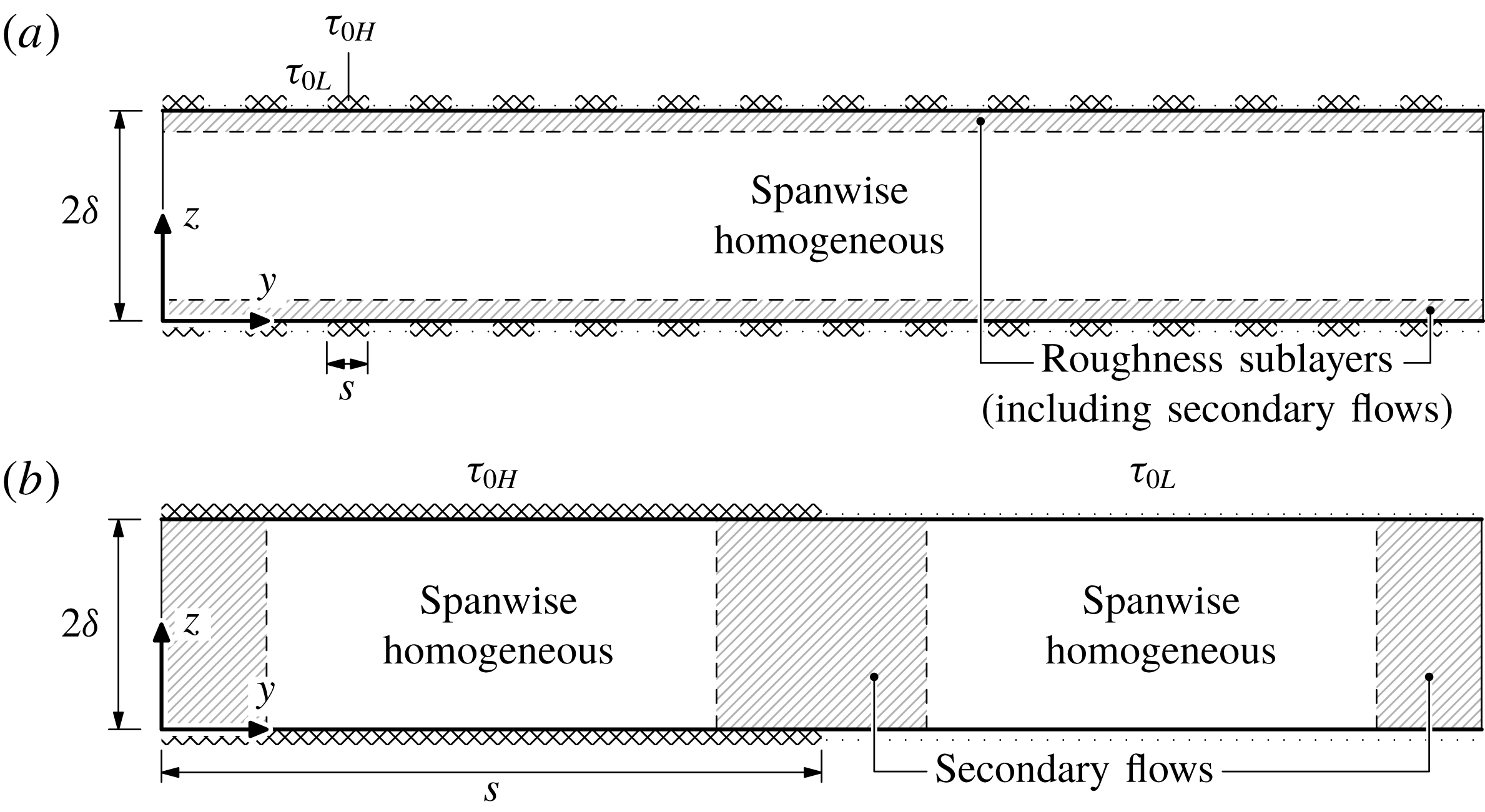
, dominate the dynamics in the bulk of the flow. In this dynamical sense, the roughness is said to be spatially uniform (figure 2
a). This regime is characterised by the two inequalities leading to (1.3). The first inequality requires the wall location
 $z$
to be far above the influence of viscosity, classically taken to be
 $30\unicode[STIX]{x1D708}/u_{\overline{\unicode[STIX]{x1D70F}}}<z$
(Tennekes & Lumley Reference Tennekes and Lumley1972), above the buffer layer. This is essentially the high Reynolds number requirement and is well understood. The second inequality requires the wall location
 $z$
to be sufficiently far above the inhomogeneous layer of the flow that is influenced by roughness, called the roughness sublayer or the blending height, the latter used in the context of spatially varying roughness (e.g. Bou-Zeid, Parlange & Meneveau Reference Bou-Zeid, Parlange and Meneveau2007). That is, above the blending height, the local defects,
 $U(y,\unicode[STIX]{x1D6FF})-U(y,z)$
, for all
 $y$
locations are identical. The requirement in terms of
 $s$
is less familiar but the version in terms of
 $k$
is often quoted as 2–
 $3k<z$
(Jiménez Reference Jiménez2004) and
 $5k<z$
(Flack, Schultz & Connelly Reference Flack, Schultz and Connelly2007), depending on the specific roughness geometry. The present idealisation in figure 1 highlights the point that a lateral scale of roughness can be important in its own right, especially for low-aspect-ratio (
 $k/s\ll 1$
) roughness. Combining
 $s\ll z$
with the implicit
 $z<\unicode[STIX]{x1D6FF}$
, the spatially uniform regime can be delineated as
 $s\ll \unicode[STIX]{x1D6FF}$
, see figure 2(a). This regime is realised, for example, in superhydrophic surfaces (Jelly et al.
Reference Jelly, Jung and Zaki2014).
Cross-section of channel, illustrating the flow structure of the (a) spatially uniform,
 $s\ll \unicode[STIX]{x1D6FF}$
, and (b) spatially varying,
 $s\gg \unicode[STIX]{x1D6FF}$
, regimes. The longitudinal (
 $x$
-direction) flow is out of the page.

When
 $s\approx \unicode[STIX]{x1D6FF}$
or
 $\unicode[STIX]{x1D6FF}\ll s$
, similarity of the global defect can no longer be expected. However, similarity of the local defect with the local shear stress can arise under certain conditions. To see this, consider now the local mean velocity defect
 $U(y,\unicode[STIX]{x1D6FF})-U(y,z)$
at wall distance
 $z$
and lateral station
 $y$
relative to a high-to-low stress jump located at
 $y_{0}$
. Dimensional considerations lead to the following general form,
 $$\begin{eqnarray}\displaystyle \frac{U(y,\unicode[STIX]{x1D6FF})-U(y,z)}{u_{\unicode[STIX]{x1D70F}}(y)}=\unicode[STIX]{x1D719}\left(\frac{y-y_{0}}{\unicode[STIX]{x1D6FF}},\frac{z}{\unicode[STIX]{x1D6FF}},\frac{z}{\unicode[STIX]{x1D708}/u_{\unicode[STIX]{x1D70F}}(y)},\frac{s}{\unicode[STIX]{x1D6FF}},\frac{\unicode[STIX]{x1D70F}_{0H}}{\unicode[STIX]{x1D70F}_{0L}}\right), & & \displaystyle\end{eqnarray}$$
where
 $u_{\unicode[STIX]{x1D70F}}(y)$
is
 $u_{\unicode[STIX]{x1D70F}H}\equiv (\unicode[STIX]{x1D70F}_{0H}/\unicode[STIX]{x1D70C})^{1/2}$
for
 $y<y_{0}$
and
 $u_{\unicode[STIX]{x1D70F}L}\equiv (\unicode[STIX]{x1D70F}_{0L}/\unicode[STIX]{x1D70C})^{1/2}$
for
 $y>y_{0}$
. If
 $s\approx \unicode[STIX]{x1D6FF}$
, this full list of parameters must be retained. However, if
 $\unicode[STIX]{x1D6FF}\ll s$
so that stations
 $y$
exist that are several outer-layer thicknesses
 $\unicode[STIX]{x1D6FF}$
away from a stress jump, i.e.
 $\unicode[STIX]{x1D6FF}\ll |y-y_{0}|$
, the local mean velocity defect is expected to take on the same one-dimensional outer-layer form
 $f$
as (1.3),
 $$\begin{eqnarray}\displaystyle \frac{U_{H}(\unicode[STIX]{x1D6FF})-U_{H}(z)}{u_{\unicode[STIX]{x1D70F}H}}=\frac{U_{L}(\unicode[STIX]{x1D6FF})-U_{L}(z)}{u_{\unicode[STIX]{x1D70F}L}}=f\left(\frac{z}{\unicode[STIX]{x1D6FF}}\right), & & \displaystyle\end{eqnarray}$$
where
 $U_{H}(\unicode[STIX]{x1D6FF})-U_{H}(z)=[U(\unicode[STIX]{x1D6FF},y)-U(z,y)]_{\unicode[STIX]{x1D6FF}\ll |y-y_{0}|}$
for
 $y<y_{0}$
(high shear stress) and
 $U_{L}(\unicode[STIX]{x1D6FF})-U_{L}(z)=[U(\unicode[STIX]{x1D6FF},y)-U(z,y)]_{\unicode[STIX]{x1D6FF}\ll |y-y_{0}|}$
for
 $y>y_{0}$
(low shear stress). In this limit, the turbulent inertial motion above the buffer layer (
 $\unicode[STIX]{x1D708}/u_{\unicode[STIX]{x1D70F}}(y)\ll z$
) deep within a uniform-stress patch (
 $\unicode[STIX]{x1D6FF}\ll |y-y_{0}|<s$
) ‘does not know’ about the flow in neighbouring patches characterised by different values of wall shear stress. This dynamical behaviour that occurs when
 $\unicode[STIX]{x1D6FF}\ll s$
invites the label, spatially varying roughness, see figure 2(b).
The orders of the constants for the inequalities that characterise the spatially uniform and spatially varying regimes,
 $s\ll \unicode[STIX]{x1D6FF}$
and
 $\unicode[STIX]{x1D6FF}\ll s$
, could depend on
 $\unicode[STIX]{x1D70F}_{0H}/\unicode[STIX]{x1D70F}_{0L}$
. Some insights into this dependence will be obtained from the present DNS data. The adherence of flow behaviour to either of these limiting regimes can be quantified by collapse in either the global defect (1.3) or local defect (1.5).
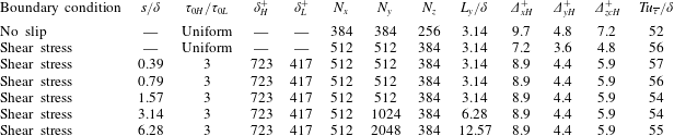
Simulation parameters.
 $\mathit{Re}_{\unicode[STIX]{x1D70F}}\equiv u_{\overline{\unicode[STIX]{x1D70F}}}\unicode[STIX]{x1D6FF}/\unicode[STIX]{x1D708}$
;
 $u_{\overline{\unicode[STIX]{x1D70F}}}\equiv (\overline{\unicode[STIX]{x1D70F}}_{0}/\unicode[STIX]{x1D70C})^{1/2}$
;
 $\overline{\unicode[STIX]{x1D70F}}_{0}\equiv (\unicode[STIX]{x1D70F}_{0H}+\unicode[STIX]{x1D70F}_{0L})/2$
, the average wall shear stress;
 $s_{H}=s_{L}=s$
, the patch width (figure 1); superscript ‘
 $+$
’ indicates viscous scaling with either
 $u_{\unicode[STIX]{x1D70F}H}/\unicode[STIX]{x1D708}$
for subscript ‘
 $H$
’ or
 $u_{\unicode[STIX]{x1D70F}L}/\unicode[STIX]{x1D708}$
for subscript ‘
 $L$
’, e.g.
 $\unicode[STIX]{x1D6FF}_{H}^{+}=\unicode[STIX]{x1D6FF}u_{\unicode[STIX]{x1D70F}H}/\unicode[STIX]{x1D708}$
; and
 $T$
is the duration of statistics collection after initial transients are discarded.
 $\mathit{Re}_{\unicode[STIX]{x1D70F}}=590$
and
 $L_{x}/\unicode[STIX]{x1D6FF}\approx 6.28$
for all present simulations.

2 DNS set-up
The channel-flow set-up is shown in figure 1. The wall-normal direction is
 $z$
, with walls located at
 $z=0$
and
 $z=2\unicode[STIX]{x1D6FF}$
. Periodic boundary conditions are imposed in the streamwise (
 $x$
) and spanwise (
 $y$
) directions. Alternating high and low wall shear stresses,
 $\unicode[STIX]{x1D70F}_{0H}$
and
 $\unicode[STIX]{x1D70F}_{0L}$
respectively, are imposed uniformly within each patch of width
 $s$
at the walls using the shear stress (Neumann) boundary condition,
 $\unicode[STIX]{x1D708}(\unicode[STIX]{x2202}u/\unicode[STIX]{x2202}z)_{z=0}=\unicode[STIX]{x1D70F}_{0H}/\unicode[STIX]{x1D70C}$
or
 $\unicode[STIX]{x1D70F}_{0L}/\unicode[STIX]{x1D70C}$
at the bottom wall and
 $-\unicode[STIX]{x1D708}(\unicode[STIX]{x2202}u/\unicode[STIX]{x2202}z)_{z=2\unicode[STIX]{x1D6FF}}=\unicode[STIX]{x1D70F}_{0H}/\unicode[STIX]{x1D70C}$
or
 $\unicode[STIX]{x1D70F}_{0L}/\unicode[STIX]{x1D70C}$
at the top wall. The no-slip boundary condition is not satisfied. As stated in § 1, this boundary condition is meant to represent an idealised roughness with low roughness blockage (
 $k/\unicode[STIX]{x1D6FF}$
small) and without changes to the dynamic origin. This boundary condition imparts no additional length scales on the flow other than the wall unit,
 $\unicode[STIX]{x1D708}/u_{\unicode[STIX]{x1D70F}}$
, and its spatial variation. The stress pattern is mirrored across the channel centreline and spanwise wall shear stress is zero uniformly,
 $\unicode[STIX]{x1D708}(\unicode[STIX]{x2202}v/\unicode[STIX]{x2202}z)_{z=0,2\unicode[STIX]{x1D6FF}}=0$
. Note that these idealised piecewise-uniform boundary conditions do not account for variations in wall shear stress that typically occur near stress jumps in real flows due to localised secondary flow. We confirmed, in a simulation where
 $(v)_{z=0,2\unicode[STIX]{x1D6FF}}=0$
for the case
 $s/\unicode[STIX]{x1D6FF}\approx 1.57$
, that the outer relative motions are virtually indistinguishable between the free-slip and no-slip
 $v$
boundary conditions. The impermeable boundary condition
 $w_{z=0,2\unicode[STIX]{x1D6FF}}=0$
is enforced uniformly at both the walls. The uniform shear stress boundary condition was previously compared with the usual no-slip boundary condition at matched
 $\mathit{Re}_{\unicode[STIX]{x1D70F}}$
, the main finding there being that the flows above the buffer layers,
 $z^{+}\approx 30$
, are essentially similar (Chung et al.
Reference Chung, Monty and Ooi2014). This includes means, Reynolds stresses, spectrograms and higher-order moments. Whilst the outer region obeys similarity, the inner region is impacted by the choice of boundary conditions, as expected. In particular, Chung et al. (Reference Chung, Monty and Ooi2014) showed, for the synthetic uniform wall shear stress (Neumann) boundary condition, that the streamwise normal Reynolds stress peaks at the wall rather than away from the wall (their figure 2a) and that the viscous sublayer is neither linear nor logarithmic but a shifted log law still appears above
 $z^{+}\approx 30$
(their figure 1b). This number agrees with classical estimates (Tennekes & Lumley Reference Tennekes and Lumley1972) and gives an indication to the lower bound below which the present flow is sensitive and therefore specific to the way in which the wall shear stress is applied. Above the buffer layer, the present flow is expected to behave similarly to other flows with the same spatially varying wall shear stress. Data from the reference no-slip and uniform shear stress cases (first two rows of table 1) will be included where relevant to aid in interpreting the statistics at hand. The wall shear stress boundary condition, in combination with the Navier–Stokes equations, are impervious to arbitrary Galilean transformations in the wall-parallel plane. In practice, a frame of reference must be chosen; here, it is chosen such that the bulk wall-parallel velocity is zero, which reduces numerical dispersion errors (Bernardini et al.
Reference Bernardini, Pirozzoli, Quadrio and Orlandi2013). It is important to only refer to Galilean-invariant statistics such as velocity differences or fluctuations, which are unambiguous and unaffected by the arbitrary frame of reference of the present simulations.
A parametric sweep for
 $s/\unicode[STIX]{x1D6FF}\approx 0.39$
–6.28 is performed at the matched friction Reynolds number,
 $\mathit{Re}_{\unicode[STIX]{x1D70F}}\equiv u_{\overline{\unicode[STIX]{x1D70F}}}\unicode[STIX]{x1D6FF}/\unicode[STIX]{x1D708}=590$
, where the friction velocity
 $u_{\overline{\unicode[STIX]{x1D70F}}}$
is based on the average wall shear stress
 $\overline{\unicode[STIX]{x1D70F}}_{0}\equiv (\unicode[STIX]{x1D70F}_{0H}+\unicode[STIX]{x1D70F}_{0L})/2$
. The stress ratio is fixed
 $\unicode[STIX]{x1D70F}_{0H}/\unicode[STIX]{x1D70F}_{0L}=3$
for the cases here with stress variations. The simulations are well resolved, set by the wall unit of the high shear stress patch where the finest scales are expected to be smaller,
 $\unicode[STIX]{x1D6E5}_{x}<8.9\unicode[STIX]{x1D708}/u_{\unicode[STIX]{x1D70F}H}$
,
 $\unicode[STIX]{x1D6E5}_{y}<4.4\unicode[STIX]{x1D708}/u_{\unicode[STIX]{x1D70F}H}$
and
 $\unicode[STIX]{x1D6E5}_{zc}<5.9\unicode[STIX]{x1D708}/u_{\unicode[STIX]{x1D70F}H}$
, where
 $\unicode[STIX]{x1D6E5}_{zc}$
is the largest wall-normal cell spacing at the channel centre (cf. Moser, Kim & Mansour Reference Moser, Kim and Mansour1999). The wall-normal cells are stretched with a cosine mapping. The CFL number, defined here as
 $\unicode[STIX]{x1D6E5}_{t}\text{max}\{|u|/\unicode[STIX]{x1D6E5}_{x},|v|/\unicode[STIX]{x1D6E5}_{y},|w|/\unicode[STIX]{x1D6E5}_{z}\}$
is fixed to unity, where
 $\unicode[STIX]{x1D6E5}_{t}$
is the time step size. Statistics are collected over many eddy-turnover times,
 $T\gtrsim 50\unicode[STIX]{x1D6FF}/u_{\overline{\unicode[STIX]{x1D70F}}}$
. Unlike simulations that are statistically homogeneous in the wall-parallel plane, the plane average that offers a quicker convergence cannot be used here and so the longer averaging times are required in order to obtain
 $x$
-averaged statistics at each
 $(y,z)$
location. The length of the channel domain for all simulations is
 $6.28\unicode[STIX]{x1D6FF}$
, which is just large enough (cf. Moser et al.
Reference Moser, Kim and Mansour1999; Lozano-Durán & Jiménez Reference Lozano-Durán and Jiménez2014); the width of the channel domain is
 $3.14\unicode[STIX]{x1D6FF}$
for
 $s\lesssim 1.57\unicode[STIX]{x1D6FF}$
, but increased up to
 $12.57\unicode[STIX]{x1D6FF}$
for
 $s\approx 6.28\unicode[STIX]{x1D6FF}$
in order to accommodate at least one period of high and low stress patch. This choice constrains the flow to scales narrower than
 $L_{y}/\unicode[STIX]{x1D6FF}\approx 3.14$
, 6.28 and 12.57, for the cases,
 $s/\unicode[STIX]{x1D6FF}\approx 1.57$
, 3.14 and 6.28, respectively, ruling out motions wider than
 $L_{y}$
, which may be important if large-scale phenomena, such as meandering, is of interest. Nonetheless, we expect minimal influence to scales narrower than
 $3.14\unicode[STIX]{x1D6FF}$
, which are captured in all the present simulations, and the domain width is sufficient (Lozano-Durán & Jiménez Reference Lozano-Durán and Jiménez2014) for mean statistics reported herein to be robust.
Here, DNS is performed using the fourth-order symmetry-preserving spatial discretisation of Verstappen & Veldman (Reference Verstappen and Veldman2003), along with the boundary conditions of Sanderse, Verstappen & Koren (Reference Sanderse, Verstappen and Koren2014). This spatial discretisation conserves mass, momentum and energy on a staggered grid. The semi-implicit low-storage third-order Runge–Kutta–Wray scheme (Spalart, Moser & Rogers Reference Spalart, Moser and Rogers1991) marches the equations in time and the fractional-step method (e.g. Perot Reference Perot1993) projects the intermediate velocity onto a divergence-free space. The viscous terms are treated implicitly only in the wall-normal direction (involving the inversion of a heptadiagonal matrix). This present code is written by the first author and has been used in a number of previous DNS studies of wall-bounded flows (e.g. Chung et al. Reference Chung, Monty and Ooi2014; Kozul, Chung & Monty Reference Kozul, Chung and Monty2016).
Global mean (spanwise-averaged) velocity defect in (a) linear–linear and (b) log–linear coordinates: ——, no slip; — —, uniform stress;

 $s/\unicode[STIX]{x1D6FF}=0.39$
;

 $s/\unicode[STIX]{x1D6FF}=0.79$
;

 $s/\unicode[STIX]{x1D6FF}=1.57$
;

 $s/\unicode[STIX]{x1D6FF}=3.14$
;

 $s/\unicode[STIX]{x1D6FF}=6.28$
.

3 Results and discussion
3.1 Global mean longitudinal velocity defect
First, we look for indications of the spatially uniform regime by considering the spanwise-averaged or ‘global’ longitudinal (streamwise) velocity defect, shown in figure 3. Recall that the roughness or wall shear stress can be considered spatially uniform from a dynamical point of view if the global velocity defect collapses according to (1.3). The profiles for the no-slip and uniform shear stress boundary-condition cases are also shown in figure 3, indicating collapse above the buffer layer,
 $z^{+}\gtrsim 30$
, as previously demonstrated by Chung et al. (Reference Chung, Monty and Ooi2014). This suggests that differences below this location should be considered specific to the boundary-condition treatment. Above this location, the uniform shear stress case serves as a reference such that departures away from it can be interpreted as a flow modification that is attributed to laterally varying roughness. Consider now the cases with imposed spatially varying wall shear stress. The global defect of the
 $s/\unicode[STIX]{x1D6FF}\approx 0.39$
case is virtually indistinguishable from the uniform shear stress case, suggesting that this case is in the spatially uniform regime. Increasing
 $s/\unicode[STIX]{x1D6FF}$
to 0.79 breaks outer-layer similarity such that the flow departs from the spatially uniform regime. This departure is an abrupt drop in the velocity defect through the bulk of the flow, with an approximate vertical shift in the logarithmic region seen in figure 3(b). However, this reduction in velocity defect is not monotonic. For
 $s/\unicode[STIX]{x1D6FF}\approx 0.79$
–1.57, the global defect reduces to a flatter profile before appearing to revert back towards the spatially uniform regime for
 $s/\unicode[STIX]{x1D6FF}\approx 3.14$
–6.28.
The reduction of the global defect to a flatter profile has been reported in a similar context in the experiment of Vanderwel & Ganapathisubramani (Reference Vanderwel and Ganapathisubramani2015) at
 $\mathit{Re}_{\unicode[STIX]{x1D70F}}\approx 4200\pm 400$
. There the flow is a boundary layer over streamwise-aligned protrusions, where the lateral spacing
 $S$
between the protrusions of width
 ${\mathcal{W}}$
is varied from
 $S/\unicode[STIX]{x1D6FF}\approx 0.30$
to 1.76 at fixed
 ${\mathcal{W}}/\unicode[STIX]{x1D6FF}\approx 0.15$
. They identify two behaviours: ‘fine’ spacing for
 $S/\unicode[STIX]{x1D6FF}\approx 0.30$
–0.45, where the global defects collapse, and ‘coarse’ spacing for
 $S/\unicode[STIX]{x1D6FF}\approx 0.88$
–1.76, where the global defects appear to also collapse, but are flatter relative to the ‘fine’ spacing cases, see their figure 3(a). The present DNS data are quantitatively consistent with these experiments with
 $s$
equivalent to
 $S$
. The spatially uniform regime collapses the present
 $s/\unicode[STIX]{x1D6FF}\approx 0.39$
, no-slip and uniform shear stress cases, which can be identified with the ‘fine’ spacing cases of Vanderwel & Ganapathisubramani (Reference Vanderwel and Ganapathisubramani2015). Also, the present
 $s/\unicode[STIX]{x1D6FF}\approx 0.79$
, 1.57 cases have flatter profiles, which is similar to the ‘coarse’ spacing cases of Vanderwel & Ganapathisubramani (Reference Vanderwel and Ganapathisubramani2015) except that the present
 $s/\unicode[STIX]{x1D6FF}\approx 0.79$
, 1.57 profiles do not collapse. Even so, the overwhelming similarities suggest, but does not prove, the generalisation that the flow transitions away from the spatially uniform regime somewhere between
 $s/\unicode[STIX]{x1D6FF}\approx 0.39$
–0.79 regardless of whether the flow is through a channel or a boundary layer, and independent of Reynolds number as the experiments are conducted at friction Reynolds numbers that are an order of magnitude larger than the present DNS. Further, the consistency in flow behaviour between a real experiment and the modelled boundary conditions supports the utility of the present idealised simulations for understanding flow over laterally varying roughness. Although the experiment of Vanderwel & Ganapathisubramani (Reference Vanderwel and Ganapathisubramani2015) did not consider spacings
 $S$
greater than
 $1.76\unicode[STIX]{x1D6FF}$
, the present DNS data go further to include two additional cases at
 $s/\unicode[STIX]{x1D6FF}\approx 3.14$
, 6.28, showing that the global defect appears to revert back towards the spatially uniform regime. The reasons for this peculiar non-monotonic behaviour will be made clear in the following sections.
Local defect
 $U_{\unicode[STIX]{x1D6FF}}-U\equiv U(y,\unicode[STIX]{x1D6FF})-U(y,z)$
at various lateral (
 $y$
) stations: scaled with the averaged friction velocity
 $u_{\overline{\unicode[STIX]{x1D70F}}}$
, left panels, i.e. (a,c,e,g,i); scaled with the local friction velocity
 $u_{\unicode[STIX]{x1D70F}}=u_{\unicode[STIX]{x1D70F}H}$
or
 $u_{\unicode[STIX]{x1D70F}L}$
, right panels, i.e. (b,d,f,h,j). Top to bottom,
 $s/\unicode[STIX]{x1D6FF}\approx 0.39$
, 0.79, 1.57, 3.14, 6.28; —— (black), uniform shear stress;


 $y$
in high shear stress region, dashed if within
 $\unicode[STIX]{x1D6FF}$
of stress jump; —— (blue),
 $y$
in low shear stress region, dashed if within
 $\unicode[STIX]{x1D6FF}$
of stress jump. See key at bottom.

3.2 Local mean longitudinal velocity defect
We now consider the local mean longitudinal velocity defect. In figure 4, the local defects at
 $y$
stations located at the centres of the high shear stress regions, at the centres of the low shear stress regions and at 16 evenly spaced locations between the two centres are shown, see key at the bottom of figure 4. For reference, the uniform shear stress defect and the globally averaged defect (left panels only) are also shown. The
 $y$
stations that are within
 $\unicode[STIX]{x1D6FF}$
of a stress jump
 $y_{0}$
, i.e.
 $|y-y_{0}|<\unicode[STIX]{x1D6FF}$
, are indicated by thin dashed lines without markers, while stations such that
 $|y-y_{0}|>\unicode[STIX]{x1D6FF}$
are indicated by thin solid lines without markers.
Figure 4(a,c,e,g,i) are scaled with the globally averaged friction velocity
 $u_{\overline{\unicode[STIX]{x1D70F}}}$
, that is, they are scaled in the same way as figure 3, but access to the local defects at various
 $y$
stations provide more detail of the structural changes to the flow. The plots in the left panels corroborate the dimensional intuition discussed in § 1.3 and illustrated in figure 2(a), where collapse indicates spanwise homogeneity. The flow for
 $s/\unicode[STIX]{x1D6FF}\approx 0.39$
behaves as in the spatially uniform regime that shows a statistically homogeneous region, where, above the blending height, all the local defects collapse onto the reference spatially uniform shear stress defect. In this regime, the globally averaged defect trivially collapses onto the uniform shear stress defect, and the flow dynamically does not ‘feel’ the small spacings of the lateral stress variations. For intermediate spacings
 $s/\unicode[STIX]{x1D6FF}\approx 0.79$
, 1.57 (figure 4
c,e), outer-layer homogeneity is broken and the flow no longer behaves in the spatially uniform regime. No clear similarity structure of the local defects can be concluded from these plots but the local defects average to a flatter profile compared to the reference uniform shear stress defect. For the large spacings,
 $s/\unicode[STIX]{x1D6FF}\approx 3.14$
, 6.28 (figure 4
g,i), the local defects fall into two groups depending on whether the
 $y$
stations are in the high shear stress or low shear stress regions. Despite the scatter of the local defects, the globally averaged defect (figure 3) remarkably approaches the reference uniform shear stress defect; this will be further explored in § 3.3.
The grouping of local defects into two indicates a tendency towards the spatially varying regime. As discussed in § 1.3 and illustrated in figure 2(b), the spatially varying regime can be measured by the local defect’s collapse to the form according to (1.5). That is, the local defects, scaled with the local friction velocity,
 $u_{\unicode[STIX]{x1D70F}H}$
or
 $u_{\unicode[STIX]{x1D70F}L}$
, collapse onto the functional form
 $f(z/\unicode[STIX]{x1D6FF})$
that is identical to the spatially uniform regime (1.3). Figure 4(b,d,f,h,j) show the local defects scaled with the local friction velocity. As the spacing is increased, the tendency towards collapse according to (1.5) is unequivocal. At the largest spacing
 $s/\unicode[STIX]{x1D6FF}\approx 6.28$
(figure 4
j), almost all the local defects collapse, except for a few
 $y$
stations that are near a stress jump because the influence of the neighbouring patch cannot be ignored, a behaviour anticipated in figure 2(b). These plots corroborate the physical picture that the flow above a uniform shear stress patch in the spatially varying regime is not aware of the dynamics in neighbouring patches of a different shear stress provided the patch is wide enough.
3.3 Global mean velocity defect of the spatially varying regime
To understand why the global defect appears to approach the uniform shear stress defect in the spatially varying regime (
 $s\gg \unicode[STIX]{x1D6FF}$
), consider the limiting case where each uniform-stress patch is so large (
 $s_{H}$
,
 $s_{L}\gg \unicode[STIX]{x1D6FF}$
) that flow is dominated by local similarity in the sense of (1.5). In this limit, the flow regions near stress jumps make negligible contributions to the global average. Thus, we can relate the local defects to the global defect via the wall-area-weighted average (cf. Mason Reference Mason1988; Bou-Zeid et al.
Reference Bou-Zeid, Meneveau and Parlange2004),
 $$\begin{eqnarray}\displaystyle \overline{U}\sim \frac{s_{L}}{s_{L}+s_{H}}U_{L}+\frac{s_{H}}{s_{L}+s_{H}}U_{H},\quad \frac{\overline{\unicode[STIX]{x1D70F}}_{0}}{\unicode[STIX]{x1D70C}}\sim \frac{s_{L}}{s_{L}+s_{H}}\frac{\unicode[STIX]{x1D70F}_{0L}}{\unicode[STIX]{x1D70C}}+\frac{s_{H}}{s_{L}+s_{H}}\frac{\unicode[STIX]{x1D70F}_{0H}}{\unicode[STIX]{x1D70C}}. & & \displaystyle\end{eqnarray}$$
These are first rewritten, (3.1a
) in defect form and (3.1b
) in terms of friction velocities recalling the definitions,
 $u_{\overline{\unicode[STIX]{x1D70F}}}\equiv (\overline{\unicode[STIX]{x1D70F}}_{0}/\unicode[STIX]{x1D70C})^{1/2}$
,
 $u_{\unicode[STIX]{x1D70F}H}\equiv (\unicode[STIX]{x1D70F}_{0H}/\unicode[STIX]{x1D70C})^{1/2}$
and
 $u_{\unicode[STIX]{x1D70F}L}\equiv (\unicode[STIX]{x1D70F}_{0L}/\unicode[STIX]{x1D70C})^{1/2}$
:
 $$\begin{eqnarray}\displaystyle \overline{U}(\unicode[STIX]{x1D6FF})-\overline{U}(z) & {\sim} & \displaystyle \frac{s_{L}}{s_{L}+s_{H}}[U_{L}(\unicode[STIX]{x1D6FF})-U_{L}(z)]+\frac{s_{H}}{s_{L}+s_{H}}[U_{H}(\unicode[STIX]{x1D6FF})-U_{H}(z)],\end{eqnarray}$$
 $$\begin{eqnarray}\displaystyle u_{\overline{\unicode[STIX]{x1D70F}}}^{2} & {\sim} & \displaystyle \frac{s_{L}}{s_{L}+s_{H}}u_{\unicode[STIX]{x1D70F}L}^{2}+\frac{s_{H}}{s_{L}+s_{H}}u_{\unicode[STIX]{x1D70F}H}^{2}.\end{eqnarray}$$
 $s\gg \unicode[STIX]{x1D6FF}$
, including in the wake. This result is supported by dimensional considerations emulating Townsend’s leading to (1.5), as the local relative flow only sees the local friction velocity, the flow thickness and the outer-flow channel geometry, that is, the same conditions as for homogeneous channel flow. Thus, substituting the local similarity forms (1.5) into (3.2a
), dividing by the square root of (3.2b
) and rearranging, we obtain
 $$\begin{eqnarray}\displaystyle \frac{\overline{U}(\unicode[STIX]{x1D6FF})-\overline{U}(z)}{\displaystyle u_{\overline{\unicode[STIX]{x1D70F}}}/G\left(\frac{\unicode[STIX]{x1D70F}_{0H}}{\unicode[STIX]{x1D70F}_{0L}},\frac{s_{H}}{s_{L}}\right)}\sim f\left(\frac{z}{\unicode[STIX]{x1D6FF}}\right)\quad \text{where}~G=\frac{\displaystyle \left(1+\frac{s_{H}}{s_{L}}\right)^{1/2}\left(1+\frac{s_{H}}{s_{L}}\frac{\unicode[STIX]{x1D70F}_{0H}}{\unicode[STIX]{x1D70F}_{0L}}\right)^{1/2}}{\displaystyle 1+\frac{s_{H}}{s_{L}}\left(\frac{\unicode[STIX]{x1D70F}_{0H}}{\unicode[STIX]{x1D70F}_{0L}}\right)^{1/2}}. & & \displaystyle\end{eqnarray}$$
 $G$
may be interpreted as a gain factor. That is, comparing (3.3) and (1.3), the global defect of the spatially varying regime obeys the same functional form as the global defect of the spatially uniform regime provided a gain
 $G$
, the ratio of the friction velocity at large spacings relative to that at small spacings, i.e.
 $G=(u_{\overline{\unicode[STIX]{x1D70F}}})_{s\gg \unicode[STIX]{x1D6FF}}/(u_{\overline{\unicode[STIX]{x1D70F}}})_{s\ll \unicode[STIX]{x1D6FF}}$
, is applied to the global-averaged friction velocity. Figure 5(a) plots the contours of
 $G$
from (3.3b
), showing that, under the conditions of the present simulations, i.e.
 $\unicode[STIX]{x1D70F}_{0H}/\unicode[STIX]{x1D70F}_{0L}=3$
and
 $s_{H}/s_{L}=1$
,
 $G\approx 1.035$
. In other words, the global velocity defect profile for large
 $s/\unicode[STIX]{x1D6FF}$
, after multiplying by 1.035, should approach the global velocity defect profile for small
 $s/\unicode[STIX]{x1D6FF}$
. This behaviour appears to be the case for
 $s/\unicode[STIX]{x1D6FF}\approx 6.28$
(figure 4
i), comparing the global-average (circled) line and the reference uniform shear stress (solid) line. This explains the peculiar behaviour of why the global-average defect of the spatially varying regime seems to approach the global defect of the spatially uniform regime. The present calculations suggest that the two are only expected to collapse to within a gain factor
 $G$
, but
 $G$
is near unity under the present conditions.
(a) Contours of gain factor,
 $G=(u_{\overline{\unicode[STIX]{x1D70F}}})_{s\gg \unicode[STIX]{x1D6FF}}/(u_{\overline{\unicode[STIX]{x1D70F}}})_{s\ll \unicode[STIX]{x1D6FF}}$
, see (3.3b
). The cross indicates the conditions of the present simulations (
 $\unicode[STIX]{x1D70F}_{0H}/\unicode[STIX]{x1D70F}_{0L}=3$
,
 $s_{H}/s_{L}=1$
), where
 $G\approx 1.035$
. (b) Ratio of defect relative to spatially uniform limit: ——,
 $s\gg \unicode[STIX]{x1D6FF}$
limit, presently
 $1/G\approx 0.966$
; — —,
 $s\ll \unicode[STIX]{x1D6FF}$
or uniform-stress limit;

 $s/\unicode[STIX]{x1D6FF}=0.39$
;

 $s/\unicode[STIX]{x1D6FF}=0.79$
;

 $s/\unicode[STIX]{x1D6FF}=1.57$
;

 $s/\unicode[STIX]{x1D6FF}=3.14$
;

 $s/\unicode[STIX]{x1D6FF}=6.28$
.

A more sensitive diagnostic is to consider the ratio of the normalised global defect relative to the normalised spatially uniform limit (figure 5
b). In this plot, it can be clearly seen that the
 $s/\unicode[STIX]{x1D6FF}\approx 0.39$
defect behaves like the spatially uniform reference case and that the approach to the spatially varying regime by
 $s/\unicode[STIX]{x1D6FF}\approx 3.14$
, 6.28 is clear, although even
 $s/\unicode[STIX]{x1D6FF}\approx 6.28$
is not large enough according to this diagnostic. Importantly, the defect of the intermediate spacings,
 $s/\unicode[STIX]{x1D6FF}\approx 0.79$
, 1.57 undershoot the spatially varying regime, meaning that the changes from the spatially uniform to the spatially varying regime are not a mere interpolation between the two limiting behaviours. The undershoots imply a flatter profile in the bulk relative to the two limiting behaviours.
3.4 Change in global skin-friction coefficient
Before discussing the changes to the global skin-friction coefficient as observed in the present simulations, consider first the limit for large spacings of the global mean velocity profile relative to the wall
 $\overline{U}(z)-\overline{U}(0)$
. To obtain this, let us assume that the flow obeys the law-of-the-wall similarity in a local sense when
 $s/\unicode[STIX]{x1D6FF}$
is large (figure 2
b). Specifically, a local composite profile comprising the log law and a wake holds over each patch:
 $$\begin{eqnarray}\displaystyle & \displaystyle \frac{U_{H}(z)-U_{H}(0)}{u_{\unicode[STIX]{x1D70F}H}}=\frac{1}{\unicode[STIX]{x1D705}}\log \frac{z}{z_{0H}}+\frac{\unicode[STIX]{x1D6F1}}{\unicode[STIX]{x1D705}}w(z/\unicode[STIX]{x1D6FF}) & \displaystyle\end{eqnarray}$$
 $$\begin{eqnarray}\displaystyle & \displaystyle \frac{U_{L}(z)-U_{L}(0)}{u_{\unicode[STIX]{x1D70F}L}}=\frac{1}{\unicode[STIX]{x1D705}}\log \frac{z}{z_{0L}}+\frac{\unicode[STIX]{x1D6F1}}{\unicode[STIX]{x1D705}}w(z/\unicode[STIX]{x1D6FF}), & \displaystyle\end{eqnarray}$$
 $w(z/\unicode[STIX]{x1D6FF})$
is Coles’ wake function, and
 $z_{0H}$
and
 $z_{0L}$
are, respectively, the roughness lengths of the high and low shear stress regions. The roughness length is used without loss of generality. For a fully rough wall, the roughness length can be expressed in terms of the equivalent sand-grain roughness via
 $z_{0}=k_{s}\text{e}^{-\unicode[STIX]{x1D705}(8.5)}\approx 0.033k_{s}$
, for a no-slip smooth wall, the roughness length can be expressed in terms of the wall unit via
 $z_{0}=(\unicode[STIX]{x1D708}/u_{\unicode[STIX]{x1D70F}})\text{e}^{-\unicode[STIX]{x1D705}A}\approx 0.13(\unicode[STIX]{x1D708}/u_{\unicode[STIX]{x1D70F}})$
, and for the present (viscous) uniform shear stress boundary condition, the roughness length can be expressed via
 $z_{0}=(\unicode[STIX]{x1D708}/u_{\unicode[STIX]{x1D70F}})\text{e}^{-\unicode[STIX]{x1D705}(A-\unicode[STIX]{x0394}U^{+})}\approx 0.50(\unicode[STIX]{x1D708}/u_{\unicode[STIX]{x1D70F}})$
as
 $\unicode[STIX]{x0394}U^{+}\approx 3.4$
(Chung et al.
Reference Chung, Monty and Ooi2014). Repeating the wall-area-weighted average similar to (3.1) for
 $\overline{U}(z)-\overline{U}(0)$
, we obtain
 $$\begin{eqnarray}\displaystyle \frac{\overline{U}(z)-\overline{U}(0)}{\displaystyle u_{\overline{\unicode[STIX]{x1D70F}}}/G\left(\frac{\unicode[STIX]{x1D70F}_{0H}}{\unicode[STIX]{x1D70F}_{0L}},\frac{s_{H}}{s_{L}}\right)}\sim \frac{1}{\unicode[STIX]{x1D705}}\log \frac{z}{z_{\overline{0}}}+\frac{\unicode[STIX]{x1D6F1}}{\unicode[STIX]{x1D705}}w(z/\unicode[STIX]{x1D6FF}), & & \displaystyle\end{eqnarray}$$
where
 $G$
is as before in (3.3b
) and the effective roughness length is a harmonic average of the two,
 $$\begin{eqnarray}\displaystyle z_{\overline{0}}=z_{0H}^{s_{H}u_{\unicode[STIX]{x1D70F}H}/(s_{H}u_{\unicode[STIX]{x1D70F}H}+s_{L}u_{\unicode[STIX]{x1D70F}L})}z_{0L}^{s_{L}u_{\unicode[STIX]{x1D70F}L}/(s_{H}u_{\unicode[STIX]{x1D70F}H}+s_{L}u_{\unicode[STIX]{x1D70F}L})}. & & \displaystyle\end{eqnarray}$$
Presently,
 $z_{\overline{0}}\approx 0.50\unicode[STIX]{x1D708}/u_{\overline{\unicode[STIX]{x1D70F}}}$
, where
 $z_{0H}\approx 0.50\unicode[STIX]{x1D708}/u_{\unicode[STIX]{x1D70F}H}$
,
 $z_{0L}\approx 0.50\unicode[STIX]{x1D708}/u_{\unicode[STIX]{x1D70F}L}$
,
 $\unicode[STIX]{x1D70F}_{0H}/\unicode[STIX]{x1D70F}_{0L}=3$
and
 $s_{H}/s_{L}=1$
have been used. That is, there is negligible shift in the mean profile relative to the wall in the large-
 $s/\unicode[STIX]{x1D6FF}$
limit compared to the small-
 $s/\unicode[STIX]{x1D6FF}$
limit, although this may not be the case for other combinations of wall type,
 $\unicode[STIX]{x1D70F}_{0H}/\unicode[STIX]{x1D70F}_{0L}$
and
 $s_{H}/s_{L}$
. There is also negligible gain
 $G\approx 1.035$
in the slope of the log law (3.5). The change between the large-
 $s/\unicode[STIX]{x1D6FF}$
profile and the small-
 $s/\unicode[STIX]{x1D6FF}$
profile is
 $$\begin{eqnarray}\displaystyle \unicode[STIX]{x1D6E5}\{[\overline{U}-\overline{U}(0)]/u_{\overline{\unicode[STIX]{x1D70F}}}\} & \equiv & \displaystyle \{[\overline{U}-\overline{U}(0)]/u_{\overline{\unicode[STIX]{x1D70F}}}\}_{s\ll \unicode[STIX]{x1D6FF}}-\{[\overline{U}-\overline{U}(0)]/u_{\overline{\unicode[STIX]{x1D70F}}}\}_{s\gg \unicode[STIX]{x1D6FF}}\nonumber\\ \displaystyle & {\approx} & \displaystyle \left(1-{\displaystyle \frac{1}{G}}\right)\left({\displaystyle \frac{1}{\unicode[STIX]{x1D705}}}\log {\displaystyle \frac{z}{z_{0}}}+{\displaystyle \frac{\unicode[STIX]{x1D6F1}}{\unicode[STIX]{x1D705}}}w(z/\unicode[STIX]{x1D6FF})\right)\nonumber\\ \displaystyle & {\approx} & \displaystyle \left(1-{\displaystyle \frac{1}{G}}\right)\{[\overline{U}-\overline{U}(0)]/u_{\overline{\unicode[STIX]{x1D70F}}}\}_{s\ll \unicode[STIX]{x1D6FF}},\end{eqnarray}$$
where the approximation
 $z_{\overline{0}}\approx z_{0}$
, has been used.
Change, relative to the uniform shear stress flow, of (a) global mean profile and (b) global skin-friction coefficient based on centreline velocity: ——,
 $s\gg \unicode[STIX]{x1D6FF}$
limit; — —,
 $s\ll \unicode[STIX]{x1D6FF}$
or uniform-stress limit;

 $s/\unicode[STIX]{x1D6FF}=0.39$
;

 $s/\unicode[STIX]{x1D6FF}=0.79$
;

 $s/\unicode[STIX]{x1D6FF}=1.57$
;

 $s/\unicode[STIX]{x1D6FF}=3.14$
;

 $s/\unicode[STIX]{x1D6FF}=6.28$
.

Figure 6(a) shows this change in global (spanwise-averaged) mean profile relative to the wall, along with the
 $s\ll \unicode[STIX]{x1D6FF}$
and
 $s\gg \unicode[STIX]{x1D6FF}$
limits, the former is zero by definition and the latter is obtained from (3.7). The approach to the large-
 $s/\unicode[STIX]{x1D6FF}$
limit does not appear to be monotonic, but a now familiar pattern emerges. For
 $s/\unicode[STIX]{x1D6FF}\lesssim 0.39$
or the spatially uniform regime, the mean profile remains mostly unchanged, and for
 $s/\unicode[STIX]{x1D6FF}\gtrsim 3.14$
, the spatially varying regime is gradually approached, with even
 $s/\unicode[STIX]{x1D6FF}\approx 6.28$
not quite recovering the
 $s/\unicode[STIX]{x1D6FF}\gg 1$
limit. In between the two regimes
 $0.79\lesssim s/\unicode[STIX]{x1D6FF}\lesssim 1.57$
, there is an overshoot of
 $\unicode[STIX]{x1D6E5}\{[\overline{U}-\overline{U}(0)]/u_{\overline{\unicode[STIX]{x1D70F}}}\}$
in the range
 $0.4<s/\unicode[STIX]{x1D6FF}<1$
, indicating that the normalised global mean velocity profile reaches a minimum relative to the spatially uniform regime. The value of
 $\unicode[STIX]{x1D6E5}\{[\overline{U}-\overline{U}(0)]/u_{\overline{\unicode[STIX]{x1D70F}}}\}$
at
 $z=\unicode[STIX]{x1D6FF}$
is plotted in figure 6(b). Specifically, figure 6(b) shows
 $\{[\overline{U}(\unicode[STIX]{x1D6FF})-\overline{U}(0)]/u_{\overline{\unicode[STIX]{x1D70F}}}\}_{s\ll \unicode[STIX]{x1D6FF}}-\{[\overline{U}(\unicode[STIX]{x1D6FF})-\overline{U}(0)]/u_{\overline{\unicode[STIX]{x1D70F}}}\}$
. If we define
 $C_{f}$
based on the centreline velocity relative to the wall velocity,
 $\overline{U}(\unicode[STIX]{x1D6FF})-\overline{U}(0)$
, then this quantity is simply
 $\sqrt{2/C_{f}}|_{s\ll \unicode[STIX]{x1D6FF}}-\sqrt{2/C_{f}}$
. That is, a peak indicates an amplified skin-friction coefficient relative to the homogeneous case. The absolute of
 $C_{f}$
is not meant to be related to any realistic values in this study, as it is highly sensitive to the near-wall treatment, i.e. the method of imposing stress variations. Of interest here is modifications to the relative motions in the outer layer. As such, a change, relative to the homogeneous case is the appropriate quantity here. This quantity can be linked to the fractional change in the skin-friction coefficient for a given
 $s/\unicode[STIX]{x1D6FF}$
relative to the skin-friction coefficient for
 $s\ll \unicode[STIX]{x1D6FF}$
,
 $$\begin{eqnarray}\displaystyle \frac{C_{f}-C_{f}|_{s\ll \unicode[STIX]{x1D6FF}}}{C_{f}|_{s\ll \unicode[STIX]{x1D6FF}}} & = & \displaystyle \frac{1}{\displaystyle \left(1-\frac{\unicode[STIX]{x1D6E5}\{[\overline{U}(\unicode[STIX]{x1D6FF})-\overline{U}(0)]/u_{\overline{\unicode[STIX]{x1D70F}}}\}}{(2/C_{f}|_{s\ll \unicode[STIX]{x1D6FF}})^{1/2}}\right)^{2}}-1\nonumber\\ \displaystyle & {\approx} & \displaystyle (2C_{f}|_{s\ll \unicode[STIX]{x1D6FF}})^{1/2}\unicode[STIX]{x1D6E5}\{[\overline{U}(\unicode[STIX]{x1D6FF})-\overline{U}(0)]/u_{\overline{\unicode[STIX]{x1D70F}}}\},\end{eqnarray}$$
where the approximation is simply a truncated Taylor series (cf. Spalart & McLean Reference Spalart and McLean2011). Figure 6(b) shows that the fractional change in skin-friction coefficient peaks near
 $s/\unicode[STIX]{x1D6FF}\approx 1$
, higher than values in both the spatially uniform and spatially varying regimes. The value of the fractional change in skin-friction coefficient depends on
 $C_{f}|_{s\ll \unicode[STIX]{x1D6FF}}$
; in the present simulations where
 $(2/C_{f}|_{s\ll \unicode[STIX]{x1D6FF}})^{1/2}\approx 18.0$
(cf. Chung et al.
Reference Chung, Monty and Ooi2014),
 $C_{f}$
is 18.8 % greater than that of the spatially uniform regime, using the peak value of
 $\unicode[STIX]{x1D6E5}\{[\overline{U}(\unicode[STIX]{x1D6FF})-\overline{U}(0)]/u_{\overline{\unicode[STIX]{x1D70F}}}\}\approx 1.7$
. This suggests a practical rule of thumb: lateral length scales of the order of the outer-layer thickness
 $\unicode[STIX]{x1D6FF}$
should be avoided in situations where low drag is desired. Also, surfaces with lateral length scales
 ${\lesssim}0.5\unicode[STIX]{x1D6FF}$
have similar drag to uniformly rough surfaces. These predictions are consistent with Medjnoun, Vanderwel & Ganapathisubramani (Reference Medjnoun, Vanderwel and Ganapathisubramani2018).
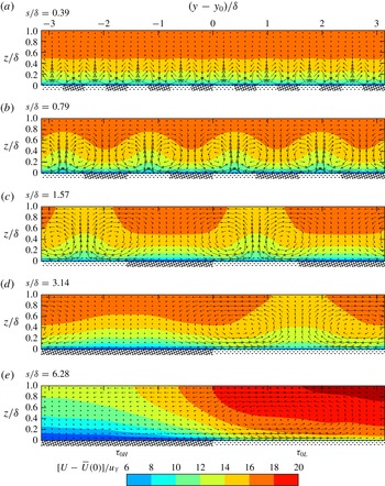
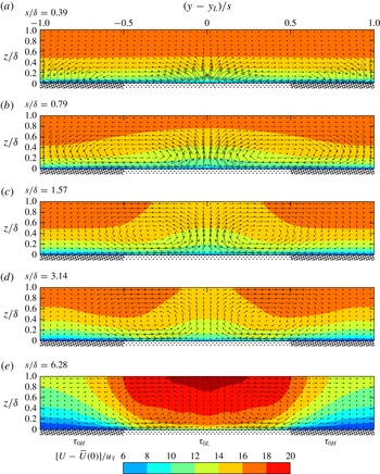
Mean (
 $xt$
-averaged) longitudinal velocity
 $U$
contours (isovels) in the cross (
 $yz$
-) plane centred on high-to-low stress jump
 $y_{0}$
. The (in-plane) secondary flow
 $[V-\overline{V}(0),W]/u_{\overline{\unicode[STIX]{x1D70F}}}$
is indicated by vectors, the lengths of which are scaled equally among the plots.

Mean (
 $xt$
-averaged) longitudinal velocity
 $U$
contours (isovels) in the cross (
 $yz$
-) plane centred on low shear stress region
 $y_{L}$
. Although there is always upwelling flow above the low shear stress region, the isovels show a sign reversal with increasing
 $s/\unicode[STIX]{x1D6FF}$
from low velocity over low shear stress for small
 $s/\unicode[STIX]{x1D6FF}$
to high velocity over low shear stress for large
 $s/\unicode[STIX]{x1D6FF}$
. The (in-plane) secondary flow
 $[V-\overline{V}(0),W]/u_{\overline{\unicode[STIX]{x1D70F}}}$
is indicated by vectors, the lengths of which are scaled equally among the plots.

3.5 Secondary flow
The results and dimensional reasoning heretofore reveal that, for the spatially uniform regime, a statistically homogeneous region occurs above the blending height, and for the spatially varying regime, a statistically homogeneous region occurs away from the stress jump. In these homogeneous regions, the identical outer-layer similarity form
 $f(z/\unicode[STIX]{x1D6FF})$
according to either (1.3) or (1.5) emerge with no mean secondary flow
 $V(y,z)=W(y,z)=0$
. Away from the homogeneous regions, i.e. near the stress jump and below the blending height, mean (
 $xt$
-averaged) secondary flow must appear. Figures 7 and 8 show the structure of the secondary flow in the vicinity of a stress jump, superimposed on contours of longitudinal isovels. Figure 7 retains the physical scaling with unity aspect ratio, which is useful for observing the increasing scale of the induced flow patterns with increasing
 $s/\unicode[STIX]{x1D6FF}$
; however, this scaling is not so useful for a global perspective because the range of spacings
 $s$
is large. For a complete perspective, figure 8 is provided where the horizontal axes are scaled with
 $s$
. The full extent of the mean cross-plane flow over a full period of low and high shear stress region is here visible for all
 $s/\unicode[STIX]{x1D6FF}$
.
Wall-normal section profiles at the centre of the low shear stress region,
 $y=y_{L}$
, of: (a)
 $W/u_{\overline{\unicode[STIX]{x1D70F}}}$
; (b)
 $[U-\overline{U}]/u_{\overline{\unicode[STIX]{x1D70F}}}$
:

 $s/\unicode[STIX]{x1D6FF}=0.39$
;

 $s/\unicode[STIX]{x1D6FF}=0.79$
;

 $s/\unicode[STIX]{x1D6FF}=1.57$
;

 $s/\unicode[STIX]{x1D6FF}=3.14$
;

 $s/\unicode[STIX]{x1D6FF}=6.28$
.

First focussing on the secondary flow, observe that it organises into a pair of counter-rotating roll motions with an upwelling region that occurs over the low stress region, independent of spacing
 $s$
. This is consistent with the link discovered by Hinze (Reference Hinze1967, Reference Hinze1973), who associate the region of low shear stress with a higher dissipation relative to production, and, in turn, to an upwelling secondary flow. The strength and coverage of the roll motion depends on the spacing of the lateral stress variation
 $s$
. At the small spacing,
 $s/\unicode[STIX]{x1D6FF}\approx 0.39$
, identified as belonging to the spatially uniform regime, the roll motion is confined near the wall below the blending height, leaving a bulk region that is virtually homogeneous. At the intermediate spacings
 $s/\unicode[STIX]{x1D6FF}\approx 0.79$
, 1.57, the roll motion strengthens and occupies the whole cross-section of the bulk flow (more noticeable for
 $s/\unicode[STIX]{x1D6FF}=1.57$
). The wall-normal velocity between the roll motions increases substantially in both magnitude and spatial occupancy over this range of
 $s/\unicode[STIX]{x1D6FF}$
(compare vector lengths at
 $y=y_{L}$
in figures 8 and 9
a). The result of this induced wall-normal velocity is a more efficient wall-normal mixing of longitudinal momentum, leading to a flatter longitudinal velocity profile as seen in figure 3. This effect on the velocity profile is consistent with the experimental observation made by Vanderwel & Ganapathisubramani (Reference Vanderwel and Ganapathisubramani2015). At large spacings,
 $s/\unicode[STIX]{x1D6FF}\approx 3.14$
, 6.28, identified as approaching the spatially varying regime, it is observed that the wall-normal velocity induced by the roll motions weakens, leading to an eventual homogeneous region between the roll motions. The roll motions generally move away from the stress jump towards the low shear stress region and remains up to
 $\unicode[STIX]{x1D6FF}$
. This explains the behaviour seen earlier, in figure 4(j) for example, where the velocity defect over almost all of the high shear stress region collapses well for large
 $s/\unicode[STIX]{x1D6FF}$
, but the same is not true for the low shear stress region. There is notably different behaviour of the spanwise velocity compared with the wall normal as the size of the spacing increases, i.e. the maximum spanwise velocity in the plane is increasing monotonically with
 $s/\unicode[STIX]{x1D6FF}$
. This means there are two different roll motions depending on
 $s/\unicode[STIX]{x1D6FF}$
; in the classification of Bradshaw (Reference Bradshaw1987): the roll motion for
 $s/\unicode[STIX]{x1D6FF}\lesssim 1.57$
is called ‘Type (b)’ or ‘identifiable streamwise vortices’, where
 $\unicode[STIX]{x2202}V/\unicode[STIX]{x2202}z$
is of the order of
 $\unicode[STIX]{x2202}W/\unicode[STIX]{x2202}y$
, while the roll motion for
 $s/\unicode[STIX]{x1D6FF}\gtrsim 3.14$
is called ‘Type (a)’ or ‘cross-flow’, where
 $\unicode[STIX]{x2202}V/\unicode[STIX]{x2202}z$
is far greater than
 $\unicode[STIX]{x2202}W/\unicode[STIX]{x2202}y$
. It is the proximity of the counter-rotating roll-motion pair that causes the behaviours seen in both
 $W$
and
 $V$
: when the roll motions are in close proximity (
 $s/\unicode[STIX]{x1D6FF}=0.79,1.57$
), the wall-normal components add together, while the spanwise components counteract each other; when the roll motions are far apart, the wall-normal components freely decay and the spanwise components are enhanced by the wall without the influence of its pair.
Turning now to the longitudinal isovels, it can be observed in figure 8 that a reversal occurs near to the surface as
 $s/\unicode[STIX]{x1D6FF}$
increases. For low
 $s/\unicode[STIX]{x1D6FF}$
we observe low longitudinal velocity over the low shear stress region, but this switches for high
 $s/\unicode[STIX]{x1D6FF}$
with high longitudinal velocity over the low shear stress region. This is more evident in figure 9(b), where profiles of the local mean relative to the spanwise-averaged longitudinal velocity are shown at the centre of the low shear stress region. The possibility for either of these two configurations was first pointed out by Hinze (Reference Hinze1973), but the conditions that favour one over the other have not been addressed in the literature. Here, it is seen that the spatially varying regime (
 $s/\unicode[STIX]{x1D6FF}\gtrsim 6.28$
) prefers the latter, a situation that is physically intuitive. If the flows over each region can be considered in isolation of neighbouring regions, it is expected that a higher longitudinal flow would be found over a low shear stress region owing to its lower resistance. However, for the small spacings
 $s/\unicode[STIX]{x1D6FF}\lesssim 3.14$
, the flows over each region cannot ignore the presence of its neighbour and, a flow arrangement develops such that a large wall-normal velocity is produced over the low shear stress region (figure 9
a). In any flow with shear in the wall-normal direction, the addition of a mean wall-normal velocity will transport low momentum from the wall and this is why a low longitudinal flow occurs over a low shear stress region as shown by Mehta & Bradshaw (Reference Mehta and Bradshaw1988). Indeed, such an arrangement of vortices has been reported, not only in laterally varying roughness studies (at spacings smaller than
 $3.14\unicode[STIX]{x1D6FF}$
) such as Willingham et al. (Reference Willingham, Anderson, Christensen and Barros2014), but also in smooth-wall, high Reynolds number wall-bounded flows, where conditional flow analyses have revealed natural high- and low-momentum regions that vary on the lateral spacing of order
 $0.5\unicode[STIX]{x1D6FF}$
(e.g. Hutchins et al.
Reference Hutchins, Monty, Ganapathisubramani, Ng and Marusic2011). The roll-motion structure is also reminiscent of that due to the linear non-normal growth mechanism (e.g. del Álamo & Jiménez Reference del Álamo and Jiménez2006; Hwang & Cossu Reference Hwang and Cossu2010). These similarities between the flow over laterally varying roughness at
 $s\lesssim 3.14\unicode[STIX]{x1D6FF}$
and smooth-wall studies suggest that the roughness variations act as a physical ‘phase lock’ that holds these linear-growth structures in space.
4 Conclusions
A numerical experiment to study the effects on wall turbulence of spanwise variations in wall shear stress is performed. Roughness effects are well known to depend on many parameters, which is the reason for limiting the varied parameters to the spanwise spacing of the high and low shear stress patches,
 $s$
, and idealising the roughness heights and origins as prescribed uniform wall shear stresses. Although further studies could be performed with variation of parameters such as the ratio of wall shear stresses (
 $\unicode[STIX]{x1D70F}_{H}/\unicode[STIX]{x1D70F}_{L}$
) or the ratio of spacings (
 $s_{H}/s_{L}$
), the current study provides sufficient insight to anticipate the effects of those parameters except, perhaps, in extreme cases.
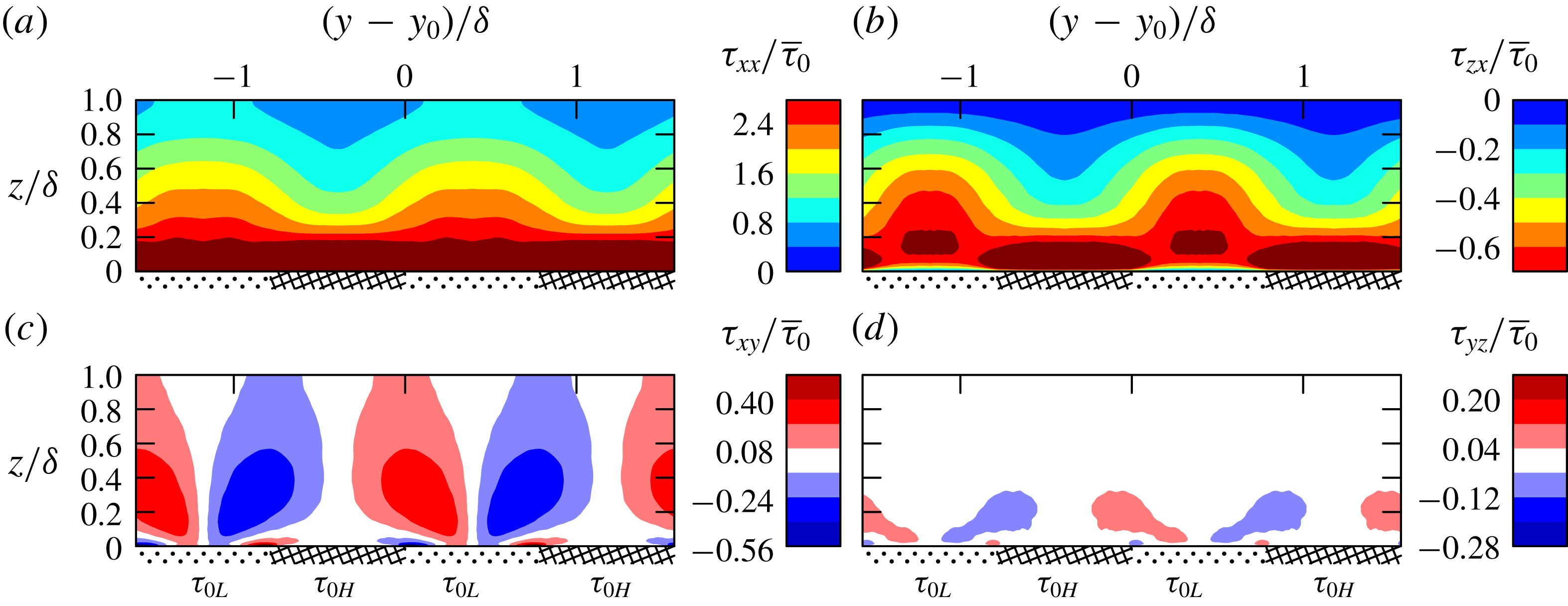
Reynolds stresses for the case
 $s/\unicode[STIX]{x1D6FF}\approx 0.79$
in the cross (
 $yz$
-) plane: (a)
 $\unicode[STIX]{x1D70F}_{xx}\equiv \unicode[STIX]{x1D70C}\overline{u^{\prime }u^{\prime }}$
, (b)
 $\unicode[STIX]{x1D70F}_{zx}\equiv \unicode[STIX]{x1D70C}\overline{w^{\prime }u^{\prime }}$
, (c)
 $\unicode[STIX]{x1D70F}_{xy}\equiv \unicode[STIX]{x1D70C}\overline{u^{\prime }v^{\prime }}$
and (d)
 $\unicode[STIX]{x1D70F}_{yz}\equiv \unicode[STIX]{x1D70C}\overline{v^{\prime }w^{\prime }}$
, where
 $u^{\prime }$
,
 $v^{\prime }$
and
 $w^{\prime }$
are fluctuations.

The predominant effect of a sharp jump from high stress to low stress (in the spanwise direction) is the generation of streamwise roll motions. For small spacings,
 $s\lesssim 0.39\unicode[STIX]{x1D6FF}$
, the roll motions produced are small and are confined so close to the wall that the flow behaves similarly (in the bulk) to a homogeneous rough- or smooth-wall flow. At very large spacings, i.e.
 $s\gtrsim 6.28\unicode[STIX]{x1D6FF}$
, the roll motions and their induced velocities are confined to the stress jump such that the bulk of the flow over the high or low shear stress regions cares only about the local shear stress below it. Between these two limits, it is shown that there are some curious, perhaps counter-intuitive, behaviours in the secondary flow. It is between the spacings of
 $0.39\lesssim s/\unicode[STIX]{x1D6FF}\lesssim 6.28$
that the roll motions become space filling and strongly interact with each other. This results in induced wall-normal velocities between the roll modes that first increase in magnitude with increasing
 $s/\unicode[STIX]{x1D6FF}$
, for
 $s/\unicode[STIX]{x1D6FF}\lesssim 1.57$
, beyond which they decrease as
 $s/\unicode[STIX]{x1D6FF}$
further increases. It is this induced wall-normal velocity that is responsible for the noted counter-intuitive flow behaviours: a breakdown of outer-layer similarity, an increased drag over the expected mean and the previously unexplained switching between low and high longitudinal velocities over the low shear stress region.
Acknowledgements
This research was supported by resources provided by The Pawsey Supercomputing Centre with funding from the Australian Government and the Government of Western Australia and by the National Computing Infrastructure (NCI), which is supported by the Australian Government. This research was partially supported under the Australian Research Council’s Discovery Projects funding scheme (project DP160103619).
Appendix. Reynolds stresses in the cross-plane
Although this paper is focussed on the similarity of mean quantities, we present in figure 10 four of the Reynolds stresses for the case
 $s/\unicode[STIX]{x1D6FF}\approx 0.79$
. Similarity with the
 $S/\unicode[STIX]{x1D6FF}\approx 0.88$
case shown in figure 6(a–d) of Vanderwel & Ganapathisubramani (Reference Vanderwel and Ganapathisubramani2015) is striking once upwelling regions are aligned. The upwelling regions correspond to low shear stresses in the present study and to the location of the protrusions in the study of Vanderwel & Ganapathisubramani (Reference Vanderwel and Ganapathisubramani2015). The structure of these Reynolds stresses are also consistent with the
 $S/\unicode[STIX]{x1D6FF}\approx 3.14$
study of Anderson et al. (Reference Anderson, Barros, Christensen and Awasthi2015) seen in their figure 4(a,c,k,g), aligning their upwelling low-roughness regions with the present upwelling low shear stress regions. That
 $\unicode[STIX]{x1D70F}_{zx}$
is more compact in the span than
 $\unicode[STIX]{x1D70F}_{xx}$
is evident in all cases. Comparing Vanderwel & Ganapathisubramani (Reference Vanderwel and Ganapathisubramani2015) and the present study, the relative magnitudes of Reynolds stresses are also similar, with maximum magnitudes indicated by maximum contour levels chosen to have identical relative ratios,
 $|\unicode[STIX]{x1D70F}_{xx}|_{max}:|\unicode[STIX]{x1D70F}_{zx}|_{max}:|\unicode[STIX]{x1D70F}_{xy}|_{max}:|\unicode[STIX]{x1D70F}_{yz}|_{max}\approx (10:2.5:2:1)\times 10^{-3}=2.8:0.7:0.56:0.28$
. The difference in absolute magnitudes is due to choice of scaling,
 $U_{\infty }^{2}$
in Vanderwel & Ganapathisubramani (Reference Vanderwel and Ganapathisubramani2015) and
 $\overline{\unicode[STIX]{x1D70F}}_{0}$
presently. The ratio of maximum contour magnitudes in Anderson et al. (Reference Anderson, Barros, Christensen and Awasthi2015) is
 $8:1.2:0.5:0.05$
, also similar, noting that their lower maximum contour magnitude for
 $\unicode[STIX]{x1D70F}_{yz}$
provide more contrast in their figure 4(g). Despite the differences between the three flows, boundary layer over protrusions at
 $\mathit{Re}_{\unicode[STIX]{x1D70F}}\approx 4200$
(Vanderwel & Ganapathisubramani Reference Vanderwel and Ganapathisubramani2015), open channel flow over wall-modelled roughness strips at atmospheric Reynolds numbers (Anderson et al.
Reference Anderson, Barros, Christensen and Awasthi2015) and channel flow over imposed stress variations at
 $\mathit{Re}_{\unicode[STIX]{x1D70F}}\approx 590$
presently, the overwhelming similarities suggest that the present boundary conditions are effective at modelling the essence of secondary flows in the outer region.