

1 Introduction
Consider the unsteady rectilinear translation of a rigid particle (with velocity  $\boldsymbol{U}(t)$, where
 $t$ is time) in an incompressible, unbounded Newtonian fluid of density
 $\unicode[STIX]{x1D70C}$ and viscosity
 $\unicode[STIX]{x1D707}$. The importance of convective fluid inertia relative to viscous forces is characterized by the Reynolds number
 $Re=\unicode[STIX]{x1D70C}U\ell /\unicode[STIX]{x1D707}$, where
 $\ell$ is the characteristic linear dimension of the particle, and
 $U$ is a representative translation speed (say the maximum of
 $|\boldsymbol{U}(t)|$). The importance of transient, or unsteady, inertia relative to viscous forces is characterized by
 $ReSl=\ell ^{2}/\unicode[STIX]{x1D708}\unicode[STIX]{x1D70F}$, where
 $\unicode[STIX]{x1D708}=\unicode[STIX]{x1D707}/\unicode[STIX]{x1D70C}$ is the kinematic viscosity,
 $\unicode[STIX]{x1D70F}$ is a time scale representative of the unsteadiness of the particle motion and
 $Sl=(\ell /U)/\unicode[STIX]{x1D70F}$ is the Strouhal number. The product
 $ReSl$ is the ratio of time required for momentum, or vorticity, to diffuse a distance
 $\ell$ (i.e.
 $\ell ^{2}/\unicode[STIX]{x1D708}$) to the imposed unsteadiness time scale
 $\unicode[STIX]{x1D70F}$. Under conditions when
 $Re\rightarrow 0$,
 $Sl\rightarrow \infty$, with
 $ReSl$ fixed, one can neglect the convective inertia term in the fluid momentum balance, but not the transient inertia (Kim & Karrila Reference Kim and Karrila1991). This gives the unsteady Stokes equations
 $$\begin{eqnarray}\unicode[STIX]{x1D70C}\frac{\unicode[STIX]{x2202}\boldsymbol{v}}{\unicode[STIX]{x2202}t}=\unicode[STIX]{x1D707}\unicode[STIX]{x1D6FB}^{2}\boldsymbol{v}-\unicode[STIX]{x1D735}p,\quad \unicode[STIX]{x1D735}\boldsymbol{\cdot }\boldsymbol{v}=0,\end{eqnarray}$$
where  $\boldsymbol{v}$ is the fluid velocity vector, and
 $p$ is the dynamic pressure. Taking the curl of (1.1) shows that vorticity,
 $\unicode[STIX]{x1D735}\times \boldsymbol{v}$, satisfies the unsteady (vector) diffusion equation. Thus, the force on an object crucially depends on how far vorticity has diffused over the time scale
 $\unicode[STIX]{x1D70F}$, a distance of order
 $\sqrt{\unicode[STIX]{x1D708}\unicode[STIX]{x1D70F}}$, relative to the length scale of the particle,
 $\ell$.
Calculation of the hydrodynamic force on an object undergoing oscillatory translation in unsteady Stokes flow is a fundamental problem in fluid mechanics. This force is relevant in the calibration of electroacoustic measurements (Loewenberg Reference Loewenberg1994), microorganism movement (Hamel et al. Reference Hamel, Fisch, Combettes, Dupuis-Williams and Baroud2011; Mathijssen et al. Reference Mathijssen, Culver, Bhamla and Prakash2019), slurry transportation (Feng & Joseph Reference Feng and Joseph1995), particle transport in turbulence (Olivieri et al. Reference Olivieri, Picano, Sardina, Ludicone and Brandt2014), chaotic advection (Daitche & Tél Reference Daitche and Tél2011) and Brownian motion (Hinch Reference Hinch1975). In the last example, the unsteady force is needed to correctly calculate the temporal decay of the velocity autocorrelation function of a Brownian particle. Specifically, inclusion of the unsteady force results in a long-time algebraic decay of the velocity autocorrelation like  $t^{-3/2}$, whereas an incorrect exponential decay is predicted if only the quasi-steady Stokes drag on the particle is considered. Note, this algebraic decay has been seen in molecular dynamics simulations (Alder & Wainwright Reference Alder and Wainwright1967) and experiments (Weitz et al. Reference Weitz, Pine, Pusey and Tough1989).
The force per unit area,  $\boldsymbol{f}(t)$, on an infinite flat plate that oscillates in its own plane at velocity
 $Re\{\boldsymbol{U}\text{e}^{-\text{i}\unicode[STIX]{x1D714}t}\}$, where
 $\unicode[STIX]{x1D714}$ is the angular frequency of oscillation,
 $\text{i}=\sqrt{-1}$ and
 $\boldsymbol{U}$ is a constant vector, is calculated in Stokes’ second problem as (Lord Rayleigh Reference Rayleigh1911)
 $$\begin{eqnarray}\boldsymbol{f}(t)=Re\left\{-\frac{\unicode[STIX]{x1D707}}{\sqrt{\unicode[STIX]{x1D708}/\unicode[STIX]{x1D714}}}\text{e}^{-\text{i}\unicode[STIX]{x03C0}/4}\boldsymbol{U}\text{e}^{-\text{i}\unicode[STIX]{x1D714}t}\right\}.\end{eqnarray}$$
The force is  $\unicode[STIX]{x03C0}/4$ out of phase with the velocity of the plate and is inversely proportional to the viscous penetration distance,
 $\sqrt{\unicode[STIX]{x1D708}/\unicode[STIX]{x1D714}}$. This phase lag is independent of the oscillation frequency. In (1.2),
 $Re\{\cdot \}$ denotes the real part of the quantity inside the brackets. Henceforth, the real part is assumed.
The unsteady force on a finite-sized particle is more complicated due to the interplay between vorticity diffusion and the body shape, which is embodied in the complex frequency parameter  $\unicode[STIX]{x1D706}^{2}=-\text{i}\ell ^{2}\unicode[STIX]{x1D714}/\unicode[STIX]{x1D708}$. For example, the unsteady force,
 $\boldsymbol{F}(t)$, on a rigid sphere of radius
 $\ell$ translating with velocity
 $\boldsymbol{U}\text{e}^{-\text{i}\unicode[STIX]{x1D714}t}$ was calculated by Stokes (Reference Stokes1851) as
 $$\begin{eqnarray}\boldsymbol{F}(t)=-6\unicode[STIX]{x03C0}\unicode[STIX]{x1D707}\boldsymbol{U}\ell \left(1+\unicode[STIX]{x1D706}+{\textstyle \frac{1}{9}}\unicode[STIX]{x1D706}^{2}\right)\text{e}^{-\text{i}\unicode[STIX]{x1D714}t}.\end{eqnarray}$$
For this special case, the force is quadratic in  $\unicode[STIX]{x1D706}$ with distinct contributions from the quasi-steady Stokes drag, Basset force and acceleration reaction. The quasi-steady Stokes drag, which corresponds to the unity term inside the brackets of (1.3), is the force on the particle due to purely viscous effects and is in phase with the particle velocity. The Basset force, which corresponds to the term
 $\unicode[STIX]{x1D706}$ inside the brackets, is
 $\unicode[STIX]{x03C0}/4$ out of phase with the particle motion; it is a perfect mix of inertial and viscous effects. The Basset force is also referred to as a ‘memory’ force as Fourier inversion of (1.3) reveals that this term is a function of the history of the particle motion (Basset Reference Basset1888). The acceleration reaction, which corresponds to the term
 $\unicode[STIX]{x1D706}^{2}$ in the brackets of (1.3), is in phase with the acceleration of the particle and is due to inviscid effects, arising from the so-called added mass due to the particle accelerating a certain volume of fluid as it changes velocity. The phase of each term is independent of frequency for a rigid sphere.
For non-spherical particles one might expect the force to remain quadratic in  $\unicode[STIX]{x1D706}$ but with different coefficients depending on particle shape. This is not the case; the force on a non-spherical particle is a far more complicated function of frequency. For a nearly spherical particle, Lawrence & Weinbaum (Reference Lawrence and Weinbaum1986) reported an additional memory term whose phase varies with frequency. Lawrence & Weinbaum (Reference Lawrence and Weinbaum1988) obtained numerical results for the force on spheroids (prolate and oblate) in axisymmetric translation and proposed a composite approximation of the force for moderate aspect ratio (
 $0.1<\unicode[STIX]{x1D716}<10$) spheroids, where
 $\unicode[STIX]{x1D716}=a/\ell$ and
 $a$ is the length of the semi-minor axis of the spheroid and, here,
 $\ell$ is its half-length. This composite approximation can be Fourier inverted in closed form to yield an expression to compute the force for arbitrary time-dependent translation. Pozrikidis (Reference Pozrikidis1989a) developed a singularity method to compute the force on moderate aspect ratio spheroids executing longitudinal or transverse oscillations. Pozrikidis (Reference Pozrikidis1989b) studied oscillatory flow past spheroids, dumbbells and biconcave disks using the boundary integral method. The added mass and Basset force for finite length, axisymmetric cylinders and spheroids were numerically computed using a boundary integral formulation by Loewenberg (Reference Loewenberg1993). Zhang & Stone (Reference Zhang and Stone1998) solved for the unsteady force on disks and used a reciprocal theorem to compute the force and torque on nearly spherical particles. Kang & Leal (Reference Kang and Leal1988) calculated the unsteady drag on a spherical drop: again, an additional memory term arises due to the mobile interface, even though the drop is spherical. Premlata & Wei (Reference Premlata and Wei2019) showed that allowing for surface slip on a rigid sphere also results in an additional memory term. Dehghani & Narsimhan (Reference Dehghani and Narsimhan2019) quantified the unsteady force on a drop with a linear viscoelastic membrane, which has the same functional form as a clean drop, provided that the viscosity of the drop is replaced by an effective, frequency-dependent viscosity that depends on the viscoelastic moduli of the membrane. In all these cases, the frequency-dependent force is far more complicated than (1.3). Evidently, the force on an oscillating, rigid sphere is a special result; in general, the unsteady force in oscillatory translation is a complicated function of frequency, due to the interplay of vorticity diffusion and the anisotropic body geometry, or surface boundary conditions.
In this work, we quantify the unsteady force on a axisymmetric, slender particle executing longitudinal or transverse oscillations. Specifically, asymptotic expansions for the force are constructed as  $\unicode[STIX]{x1D716}=a/\ell \rightarrow 0$; here,
 $a$ is the characteristic cross-sectional width of the particle and
 $\ell$ is the half-length. We compare our asymptotic results for the frequency-dependent force to solutions of the unsteady Stokes equations around a prolate spheroid (
 $\unicode[STIX]{x1D716}=0.1$) from Lawrence & Weinbaum (Reference Lawrence and Weinbaum1988) for the longitudinal case (via eigenfunction expansions) and Pozrikidis (Reference Pozrikidis1989a) for the transverse case (via boundary integral computations), finding good agreement. The asymptotic results yield a physical understanding of the behaviour of the force across the entire frequency spectrum, which is difficult to gain from a purely numerical solution.
In § 2 we compute the force on a slender particle undergoing longitudinal oscillation. In § 3 we compute the force on a slender particle undergoing transverse oscillation. A concluding discussion is offered in § 4.
2 Unsteady force for longitudinal oscillation
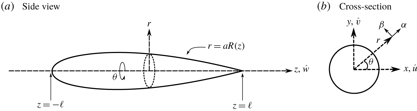
Consider a rigid, axisymmetric particle undergoing longitudinal oscillation in an otherwise stagnant, unbounded fluid (figure 1). The particle is slender,  $\unicode[STIX]{x1D716}=a/\ell \ll 1$, and the longitudinal profile of its cross-section is given by
 $aR(z)$, where
 $R(z)$ is a dimensionless shape function that varies on the scale of
 $\ell$ and vanishes at the ends of the body. The particle has velocity
 $\hat{\boldsymbol{U}}\text{e}^{-\text{i}\unicode[STIX]{x1D714}t}$ where
 $\hat{\boldsymbol{U}}$ is the velocity vector in the direction of oscillation; e.g.
 $\hat{\boldsymbol{U}}$ is directed along
 $\boldsymbol{e}_{z}$ for longitudinal oscillation, where
 $\boldsymbol{e}_{z}$ is the unit vector along the
 $z$-axis. Since the unsteady Stokes equations are linear, the fluid velocity
 $\boldsymbol{v}$ and dynamic pressure
 $p$ vary with the frequency of the particle translation; thus, we write
 $\boldsymbol{v}=\hat{\boldsymbol{v}}\text{e}^{-\text{i}\unicode[STIX]{x1D714}t}$ and
 $p=\hat{p}\text{e}^{-\text{i}\unicode[STIX]{x1D714}t}$. The dimensionless, Fourier-transformed unsteady Stokes equations are thus
 $$\begin{eqnarray}\unicode[STIX]{x1D706}^{2}\hat{\boldsymbol{v}}=\unicode[STIX]{x1D6FB}^{2}\hat{\boldsymbol{v}}-\unicode[STIX]{x1D735}\hat{p},\quad \unicode[STIX]{x1D735}\boldsymbol{\cdot }\hat{\boldsymbol{v}}=0,\end{eqnarray}$$
 $$\begin{eqnarray}\hat{\boldsymbol{v}}=\boldsymbol{e}_{z},\quad \text{on }r=\unicode[STIX]{x1D716}R(z)\text{ and }|z|\leqslant 1,\end{eqnarray}$$
 $$\begin{eqnarray}\hat{\boldsymbol{v}}\rightarrow 0\text{ and }\hat{p}\rightarrow 0\text{ as }(r^{2}+z^{2})^{1/2}\rightarrow \infty ,\end{eqnarray}$$
 $\ell$, time is normalized by
 $\ell ^{2}/\unicode[STIX]{x1D708}$, Fourier-space velocity (
 $\hat{\boldsymbol{v}}$) by
 $|\hat{\boldsymbol{U}}|\ell ^{2}/\unicode[STIX]{x1D708}$ and Fourier-space pressure (
 $\hat{p}$) by
 $\unicode[STIX]{x1D70C}|\hat{\boldsymbol{U}}|\ell$. Henceforth, all quantities are in dimensionless form unless otherwise stated.
Sketch of an axisymmetric, slender particle with a cylindrical coordinate system ( $r,\unicode[STIX]{x1D703},z$). Here,
 $R(z)$ is a dimensionless shape function which vanishes at the ends of the body. The fluid velocity components along the Cartesian axes (
 $x,y,z$) are (
 $\hat{u} ,\hat{v},{\hat{w}}$). We also denote the velocity components in the
 $r$ and
 $\unicode[STIX]{x1D703}$ directions as
 $\unicode[STIX]{x1D6FC}$ and
 $\unicode[STIX]{x1D6FD}$, respectively. For longitudinal oscillations the particle moves along the
 $z$-axis and for transverse oscillations along the
 $x$-axis.

2.1 Low-frequency longitudinal oscillation
We first consider the distinguished limit  $\unicode[STIX]{x1D716}\rightarrow 0$ with
 $|\unicode[STIX]{x1D706}|$ fixed, which we refer to as the ‘low-frequency’ regime. Here, the time for momentum to diffuse over the length of the particle is comparable to the period of oscillation. This implies that the flow on the scale of the cross-section is quasi-steady. Unsteady effects are only observed on the scale of the particle length, where the details of the cross-sectional profile are lost and the particle appears as an unsteady line source of momentum.
The flows in these two regions – i.e. on the scale of the particle cross-section and the particle length – are treated separately using slender-body theory. The first (‘inner’) region is a distance from the particle on the scale of the cross-sectional width; hence, we define an inner coordinate  $\unicode[STIX]{x1D70C}=r/\unicode[STIX]{x1D716}=O(1)$ as
 $\unicode[STIX]{x1D716}\rightarrow 0$. The second (‘outer’) region corresponds to
 $r=O(1)$. The continuity equation in the inner region implies that the cross-sectional velocity components,
 $\hat{u}$ and
 $\hat{v}$, are
 $O(\unicode[STIX]{x1D716})$ smaller than the axial velocity,
 ${\hat{w}}$, and the latter is at most
 $O(1)$ from (2.1b). From (2.1a), the axial momentum balance in the inner region is
 $$\begin{eqnarray}\frac{1}{\unicode[STIX]{x1D70C}}\frac{\unicode[STIX]{x2202}}{\unicode[STIX]{x2202}\unicode[STIX]{x1D70C}}\left(\unicode[STIX]{x1D70C}\frac{\unicode[STIX]{x2202}{\hat{w}}}{\unicode[STIX]{x2202}\unicode[STIX]{x1D70C}}\right)+\unicode[STIX]{x1D716}^{2}\frac{\unicode[STIX]{x2202}^{2}{\hat{w}}}{\unicode[STIX]{x2202}z^{2}}-\unicode[STIX]{x1D716}^{2}\frac{\unicode[STIX]{x2202}\hat{p}}{\unicode[STIX]{x2202}z}=\unicode[STIX]{x1D716}^{2}\unicode[STIX]{x1D706}^{2}{\hat{w}}.\end{eqnarray}$$
Since  $\unicode[STIX]{x1D716}\rightarrow 0$ with
 $|\unicode[STIX]{x1D706}|$ fixed, equation (2.2) reduces to the standard axial momentum balance in slender-body theory of quasi-steady Stokes flow (Batchelor Reference Batchelor1970)
 $$\begin{eqnarray}\frac{1}{\unicode[STIX]{x1D70C}}\frac{\unicode[STIX]{x2202}}{\unicode[STIX]{x2202}\unicode[STIX]{x1D70C}}\left(\unicode[STIX]{x1D70C}\frac{\unicode[STIX]{x2202}{\hat{w}}}{\unicode[STIX]{x2202}\unicode[STIX]{x1D70C}}\right)=0,\end{eqnarray}$$
which has the solution (Batchelor Reference Batchelor1970)
 $$\begin{eqnarray}{\hat{w}}=\frac{f(z;\unicode[STIX]{x1D716})}{2\unicode[STIX]{x03C0}}\ln \left(\frac{\unicode[STIX]{x1D70C}}{R(z)}\right)+1.\end{eqnarray}$$
Here,  $f=f(z;\unicode[STIX]{x1D716})$ is the dimensionless axial force per unit length on the particle in the
 $z$-direction (normalized by
 $\unicode[STIX]{x1D707}|\hat{\boldsymbol{U}}|$), such that the total (dimensionless) force is
 $F_{L}=\int _{-1}^{1}f(z;\unicode[STIX]{x1D716})\,\text{d}z$, where the subscript
 $L$ stands for ‘low frequency’. We rewrite (2.4) in terms of the outer coordinate
 $r$ as
 $$\begin{eqnarray}{\hat{w}}=\frac{f(z;\unicode[STIX]{x1D716})}{2\unicode[STIX]{x03C0}}\left[\ln \left(\frac{r}{R(z)}\right)+\ln \left(\frac{1}{\unicode[STIX]{x1D716}}\right)\right]+1,\end{eqnarray}$$
which suggests that  $f(z;\unicode[STIX]{x1D716})=O[1/\text{ln}(1/\unicode[STIX]{x1D716})]$ to leading order, to ensure that the outer flow is bounded as
 $\unicode[STIX]{x1D716}\rightarrow 0$. Thus, the leading-order axial force per unit length is
 $f=-2\unicode[STIX]{x03C0}/\text{ln}(1/\unicode[STIX]{x1D716})$, where the coefficient
 $-2\unicode[STIX]{x03C0}$ is chosen to ensure that the velocity in the outer region is asymptotically small in
 $\unicode[STIX]{x1D716}$ (by cancelling the unity at the right of (2.5)), and the minus sign indicates the force is in the opposite direction of the particle velocity. The leading axial force on the particle is the same as in slender-body theory of quasi-steady Stokes flow, which is unsurprising since the unsteadiness of the flow in the inner region is negligible. The above analysis suggests the logarithmic, or weak, expansion
 $$\begin{eqnarray}f(z;\unicode[STIX]{x1D716})=-\frac{2\unicode[STIX]{x03C0}}{\ln (1/\unicode[STIX]{x1D716})}+\frac{f_{2}(z)}{\ln ^{2}(1/\unicode[STIX]{x1D716})}+O\left[\frac{1}{\ln ^{3}(1/\unicode[STIX]{x1D716})}\right].\end{eqnarray}$$
An alternative to the weak expansion is to derive an integral equation for the axial force per unit length,  $f(z;\unicode[STIX]{x1D716})$, which could then be solved numerically. The latter approach would allow one to obtain
 $f$ within an error that is algebraically small in
 $\unicode[STIX]{x1D716}$.
Combining (2.5) and (2.6), the inner axial velocity in terms of the outer coordinate is
 $$\begin{eqnarray}{\hat{w}}=-\frac{\ln (r)}{\ln (1/\unicode[STIX]{x1D716})}+\frac{1}{\ln (1/\unicode[STIX]{x1D716})}\left[\ln (R(z))+\frac{f_{2}}{2\unicode[STIX]{x03C0}}\right]+O\left[\frac{1}{\ln ^{2}(1/\unicode[STIX]{x1D716})}\right].\end{eqnarray}$$
Thus in the outer region,  $r=O(1)$, we expand the velocity and pressure as
 $$\begin{eqnarray}\hat{\boldsymbol{v}}=\frac{\hat{\boldsymbol{v}}_{1}}{\ln (1/\unicode[STIX]{x1D716})}+O\left[\frac{1}{\ln ^{2}(1/\unicode[STIX]{x1D716})}\right]\quad \text{and}\quad \hat{p}=\frac{\hat{p}_{1}}{\ln (1/\unicode[STIX]{x1D716})}+O\left[\frac{1}{\ln ^{2}(1/\unicode[STIX]{x1D716})}\right]\end{eqnarray}$$
since (2.7) shows that the outer velocity disturbance is  $O[1/\text{ln}(1/\unicode[STIX]{x1D716})]$ to leading order. The particle appears as a line segment of zero width on the scale of the outer region. Hence, we construct the
 $\hat{\boldsymbol{v}}_{1}$ field as a line distribution of oscillating Stokeslets, i.e. the fundamental solution to (2.1a). Thus,
 $$\begin{eqnarray}\hat{\boldsymbol{v}}_{1}=\frac{1}{8\unicode[STIX]{x03C0}}\int _{-1}^{1}\boldsymbol{G}(\boldsymbol{x},\boldsymbol{x}_{0})\boldsymbol{\cdot }[h(z_{0})\boldsymbol{e}_{z}]\,\text{d}z_{0},\end{eqnarray}$$
where  $h$ is the strength of the unsteady Stokeslet at a location
 $z_{0}$ along the axis of the particle, and
 $\boldsymbol{G}$ is the Green function for an oscillating Stokeslet (Kim & Karrila Reference Kim and Karrila1991)
 $$\begin{eqnarray}\boldsymbol{G}(\boldsymbol{x},\boldsymbol{x}_{0})=\frac{A\boldsymbol{I}}{|\hat{\boldsymbol{x}}|}+\frac{B\;\hat{\boldsymbol{x}}\hat{\boldsymbol{x}}}{|\hat{\boldsymbol{x}}|^{3}},\end{eqnarray}$$
where  $\hat{\boldsymbol{x}}$ is the difference of
 $\boldsymbol{x}$, the position vector in cylindrical coordinates
 $\boldsymbol{x}=r\boldsymbol{e}_{r}+z\boldsymbol{e}_{z}$, and
 $\boldsymbol{x}_{0}$, the position of each oscillating Stokeslet
 $\boldsymbol{x}_{0}=z_{0}\boldsymbol{e}_{z}$. The coefficients
 $A$ and
 $B$ are
 $$\begin{eqnarray}\left.\begin{array}{@{}c@{}}\displaystyle A(\boldsymbol{x},\boldsymbol{x}_{0})=2\text{e}^{-\unicode[STIX]{x1D706}|\hat{\boldsymbol{x}}|}[1+(\unicode[STIX]{x1D706}|\hat{\boldsymbol{x}}|)^{-1}+(\unicode[STIX]{x1D706}|\hat{\boldsymbol{x}}|)^{-2}]-2(\unicode[STIX]{x1D706}|\hat{\boldsymbol{x}}|)^{-2},\\ \displaystyle B(\boldsymbol{x},\boldsymbol{x}_{0})=-2\text{e}^{-\unicode[STIX]{x1D706}|\hat{\boldsymbol{x}}|}[1+3(\unicode[STIX]{x1D706}|\hat{\boldsymbol{x}}|)^{-1}+3(\unicode[STIX]{x1D706}|\hat{\boldsymbol{x}}|)^{-2}]+6(\unicode[STIX]{x1D706}|\hat{\boldsymbol{x}}|)^{-2}.\end{array}\right\}\end{eqnarray}$$
We only need the axial velocity component in the outer region,  ${\hat{w}}_{1}$, for matching with the inner region. Thus, using (2.9)–(2.11), we have
 $$\begin{eqnarray}{\hat{w}}_{1}=\frac{1}{8\unicode[STIX]{x03C0}}\int _{-1}^{1}\left[\frac{Ah(z_{0})}{[r^{2}+(z-z_{0})^{2}]^{1/2}}+\frac{(z-z_{0})^{2}Bh(z_{o})}{[r^{2}+(z-z_{0})^{2}]^{3/2}}\right]\text{d}z_{0}.\end{eqnarray}$$
We need the limit of (2.12) as  $r\rightarrow 0$ to match the inner solution (2.7); however, the integrals in (2.12) are singular as
 $r\rightarrow 0$. To evaluate this limit, each integral can be split into two integrals, one singular and one regular as
 $r\rightarrow 0$ through the method of Schnitzer (Reference Schnitzer2015): see equations (3.9) and (3.10), and the accompanying discussion in that paper. Asymptotic approximations for the singular integrals were computed by Batchelor (Reference Batchelor1970); the final result is
 $$\begin{eqnarray}{\hat{w}}_{1}=\frac{h(z)}{4\unicode[STIX]{x03C0}}\left[2\ln \left(\frac{2(1-z^{2})^{1/2}}{r}\right)-1\right]+\frac{1}{8\unicode[STIX]{x03C0}}\int _{-1}^{1}\frac{(A+B)h(z_{0})-2h(z)}{|z-z_{0}|}\,\text{d}z_{0}+o(1),\end{eqnarray}$$
where now in (2.13)  $A$ and
 $B$ have the argument
 $\unicode[STIX]{x1D706}|z-z_{0}|$. Matching (2.7) and (2.13) first gives a uniform source density
 $h(z)=2\unicode[STIX]{x03C0}$. Second, matching gives the
 $O[\ln ^{-2}(1/\unicode[STIX]{x1D716})]$ correction to the force per unit length,
 $$\begin{eqnarray}\frac{f_{2}}{2\unicode[STIX]{x03C0}}=\ln \left[\frac{2(1-z^{2})^{1/2}}{R(z)}\right]-\frac{1}{2}+\frac{1}{4}\int _{-1}^{1}\frac{A+B-2}{|z-z_{0}|}\,\text{d}z_{0}.\end{eqnarray}$$
Upon integrating over the length of the particle, the total force is
 $$\begin{eqnarray}F_{L}=-\frac{4\unicode[STIX]{x03C0}}{\ln (1/\unicode[STIX]{x1D716})}+\frac{F_{2}}{\ln ^{2}(1/\unicode[STIX]{x1D716})}+O\left[\frac{1}{\ln ^{3}(1/\unicode[STIX]{x1D716})}\right],\end{eqnarray}$$
in which
 $$\begin{eqnarray}\displaystyle F_{2} & = & \displaystyle 2\unicode[STIX]{x03C0}\left[\int _{-1}^{1}\ln \left[\frac{2(1-z^{2})^{1/2}}{R(z)}\right]-\frac{1}{2}\,\text{d}z\right]\nonumber\\ \displaystyle & & \displaystyle +\,\unicode[STIX]{x03C0}\left[2-4\unicode[STIX]{x1D6FE}+4(1-\ln (2\unicode[STIX]{x1D706}))+\left(\frac{1-2\unicode[STIX]{x1D706}-\text{e}^{-2\unicode[STIX]{x1D706}}}{\unicode[STIX]{x1D706}^{2}}\right)+\frac{2}{\unicode[STIX]{x1D706}}(\text{e}^{-2\unicode[STIX]{x1D706}}-1)-4E_{1}(2\unicode[STIX]{x1D706})\right].\nonumber\\ \displaystyle & & \displaystyle\end{eqnarray}$$
In (2.16),  $E_{1}(2\unicode[STIX]{x1D706})=\int _{2\unicode[STIX]{x1D706}}^{\infty }s^{-1}\text{e}^{-s}\,\text{d}s$ is the exponential integral and
 $\unicode[STIX]{x1D6FE}=0.577\ldots$ is the Euler–Mascheroni constant.
The low-frequency limit of (2.16) is
 $$\begin{eqnarray}\frac{F_{2}}{4\unicode[STIX]{x03C0}}=\frac{1}{2}\left(\int _{-1}^{1}\left[\ln \left[\frac{2(1-z^{2})^{1/2}}{R(z)}\right]-\frac{1}{2}\right]\text{d}z\right)-\frac{2}{3}\unicode[STIX]{x1D706}+O(\unicode[STIX]{x1D706}^{2}).\end{eqnarray}$$
Lawrence & Weinbaum (Reference Lawrence and Weinbaum1988) have shown that the force on an arbitrary particle at low frequency is
 $$\begin{eqnarray}\boldsymbol{F}=-6\unicode[STIX]{x03C0}\hat{\boldsymbol{U}}\boldsymbol{\cdot }\left[\unicode[STIX]{x1D63C}+\unicode[STIX]{x1D706}\,\unicode[STIX]{x1D63C}\boldsymbol{\cdot }\unicode[STIX]{x1D63C}+O(\unicode[STIX]{x1D706}^{2})\right],\end{eqnarray}$$
where  $\unicode[STIX]{x1D63C}$ is the dimensionless resistance tensor coupling force to translation in quasi-steady Stokes flow. From slender-body theory (Batchelor Reference Batchelor1970),
 $$\begin{eqnarray}\unicode[STIX]{x1D63C}=\frac{2}{3\ln (1/\unicode[STIX]{x1D716})}\left[\boldsymbol{e}_{z}\boldsymbol{e}_{z}+2\left(\boldsymbol{I}-\boldsymbol{e}_{z}\boldsymbol{e}_{z}\right)\right]+O\left[\frac{1}{\ln ^{2}(1/\unicode[STIX]{x1D716})}\right].\end{eqnarray}$$
Combining (2.18) with (2.19), the low-frequency approximation of the force for longitudinal oscillation ( $\hat{\boldsymbol{U}}=\boldsymbol{e}_{z}$) is
 $$\begin{eqnarray}\boldsymbol{F}=-\frac{4\unicode[STIX]{x03C0}}{\ln (1/\unicode[STIX]{x1D716})}\left[1+\frac{2\unicode[STIX]{x1D706}}{3\ln (1/\unicode[STIX]{x1D716})}\right]\boldsymbol{e}_{z}+O(\unicode[STIX]{x1D706}^{2}).\end{eqnarray}$$
The  $O(\unicode[STIX]{x1D706})$ contribution to (2.20) is consistent with that of (2.17). Note, the
 $\unicode[STIX]{x1D706}$-independent term in (2.17) is contained in the
 $O[1/\text{ln}^{2}(1/\unicode[STIX]{x1D716})]$ error of (2.19) and therefore does not appear in (2.20).
As  $|\unicode[STIX]{x1D706}|\rightarrow \infty$ we find
 $$\begin{eqnarray}\frac{F_{2}}{4\unicode[STIX]{x03C0}}=\frac{1}{2}\left(\int _{-1}^{1}\left[\ln \left[\frac{2(1-z^{2})^{1/2}}{R(z)}\right]-\frac{1}{2}\right]\text{d}z\right)+\frac{3}{2}-\unicode[STIX]{x1D6FE}-\ln (2\unicode[STIX]{x1D706})+O(\unicode[STIX]{x1D706}^{-1}).\end{eqnarray}$$
Consequently, the force on the particle
 $$\begin{eqnarray}\frac{F}{4\unicode[STIX]{x03C0}}=-\frac{1}{\ln (1/\unicode[STIX]{x1D716})}-\frac{\ln (\unicode[STIX]{x1D706})}{\ln ^{2}(1/\unicode[STIX]{x1D716})}+\cdots \,.\end{eqnarray}$$
Therefore, the correction term is comparable to the leading-order term when  $\unicode[STIX]{x1D716}|\unicode[STIX]{x1D706}|=O(1)$, signifying a loss of uniformity in the expansion. Therefore, we may extend the range of validity of the low-frequency expansion from
 $\unicode[STIX]{x1D716}\rightarrow 0$ with
 $|\unicode[STIX]{x1D706}|$ fixed to
 $\unicode[STIX]{x1D716}\rightarrow 0$ and
 $\unicode[STIX]{x1D716}|\unicode[STIX]{x1D706}|\ll 1$. Physically, for
 $\unicode[STIX]{x1D716}|\unicode[STIX]{x1D706}|=O(1)$ we cannot neglect unsteadiness in the inner region, as the momentum diffusion time over the cross-sectional width is now comparable to the period of oscillation. This prompts a new asymptotic approximation in a ‘moderate-frequency’ regime.
2.2 Moderate-frequency longitudinal oscillation
Moderate-frequency oscillations correspond to the distinguished limit  $\unicode[STIX]{x1D716}\rightarrow 0$ with
 $\unicode[STIX]{x1D716}|\unicode[STIX]{x1D706}|=O(1)$. Here, momentum cannot diffuse past the inner region before the particle switches direction. Therefore, we must take into account the unsteadiness of the flow in the inner region. Thus, the leading-order axial momentum balance in the inner region (2.2) becomes
 $$\begin{eqnarray}\frac{1}{\unicode[STIX]{x1D70C}}\frac{\unicode[STIX]{x2202}}{\unicode[STIX]{x2202}\unicode[STIX]{x1D70C}}\left(\unicode[STIX]{x1D70C}\frac{\unicode[STIX]{x2202}{\hat{w}}}{\unicode[STIX]{x2202}\unicode[STIX]{x1D70C}}\right)-\unicode[STIX]{x1D716}^{2}\unicode[STIX]{x1D706}^{2}{\hat{w}}=0.\end{eqnarray}$$
Recall, the second term in (2.23) is the Fourier transform of the time dependent inertia and is now  $O(1)$ since
 $\unicode[STIX]{x1D716}|\unicode[STIX]{x1D706}|=O(1)$, even though
 $\unicode[STIX]{x1D716}\ll 1$. The solution to (2.23) is
 $$\begin{eqnarray}{\hat{w}}(\unicode[STIX]{x1D70C},z)=\frac{K_{0}(\unicode[STIX]{x1D716}\unicode[STIX]{x1D706}\unicode[STIX]{x1D70C})}{K_{0}(\unicode[STIX]{x1D716}\unicode[STIX]{x1D706}R(z))},\end{eqnarray}$$
where  $K_{j}$ is the
 $j\text{th}$-order modified Bessel function of second kind. At large distances,
 $\unicode[STIX]{x1D70C}\gg 1$, equation (2.24) has the form
 $$\begin{eqnarray}{\hat{w}}\sim \unicode[STIX]{x1D70C}^{-1/2}R(z)^{1/2}\text{e}^{-\unicode[STIX]{x1D716}\unicode[STIX]{x1D706}[\unicode[STIX]{x1D70C}-R(z)]},\end{eqnarray}$$
which represents Stokes waves with amplitude factor  $\unicode[STIX]{x1D70C}^{-1/2}$ due to the transverse curvature of the body. Physically, the particle is oscillating so quickly that the fluid at
 $\unicode[STIX]{x1D70C}\sim O(\unicode[STIX]{x1D716}^{-1})$ (i.e. in the outer region) is essentially undisturbed. More precisely, the inner region contains Stokes waves whose amplitude is exponentially small in the outer region.
Using (2.24) with the continuity equation shows that there exists an  $O(\unicode[STIX]{x1D716})$ small radial velocity
 $\unicode[STIX]{x1D6FC}\boldsymbol{e}_{r}$ in the inner region (
 $\boldsymbol{e}_{r}$ is a radial unit vector in the plane of the cross-section), where
 $$\begin{eqnarray}\unicode[STIX]{x1D6FC}=\unicode[STIX]{x1D716}\frac{\text{d}R(z)}{\text{d}z}\frac{K_{1}(\unicode[STIX]{x1D716}\unicode[STIX]{x1D706}R(z))}{K_{0}(\unicode[STIX]{x1D716}\unicode[STIX]{x1D706}R(z))^{2}}\left(K_{1}(\unicode[STIX]{x1D716}\unicode[STIX]{x1D706}\unicode[STIX]{x1D70C})-\frac{R(z)}{\unicode[STIX]{x1D70C}}K_{1}(\unicode[STIX]{x1D716}\unicode[STIX]{x1D706}R(z))\right).\end{eqnarray}$$
The axial component of the traction at the particle surface is  $\boldsymbol{e}_{z}\boldsymbol{\cdot }\unicode[STIX]{x1D748}\boldsymbol{\cdot }\boldsymbol{n}$, where
 $\unicode[STIX]{x1D748}$ is the stress tensor and
 $\boldsymbol{n}=\boldsymbol{e}_{r}-\unicode[STIX]{x1D716}(\text{d}R(z)/\text{d}z)\boldsymbol{e}_{z}+O(\unicode[STIX]{x1D716}^{2})$ is the outward unit normal to the particle surface. It is readily shown that
 $$\begin{eqnarray}\boldsymbol{e}_{z}\boldsymbol{\cdot }\unicode[STIX]{x1D748}\boldsymbol{\cdot }\boldsymbol{n}=\frac{1}{\unicode[STIX]{x1D716}}\frac{\unicode[STIX]{x2202}{\hat{w}}}{\unicode[STIX]{x2202}\unicode[STIX]{x1D70C}}+\left(\hat{p}\unicode[STIX]{x1D716}\frac{\text{d}R(z)}{\text{d}z}+\frac{\unicode[STIX]{x2202}\unicode[STIX]{x1D6FC}}{\unicode[STIX]{x2202}z}-2\unicode[STIX]{x1D716}\frac{\unicode[STIX]{x2202}{\hat{w}}}{\unicode[STIX]{x2202}z}\frac{\text{d}R(z)}{\text{d}z}\right)+o(\unicode[STIX]{x1D716}),\end{eqnarray}$$
where  $\hat{p}$ is the pressure in the inner region. The traction is
 $(1/\unicode[STIX]{x1D716})(\unicode[STIX]{x2202}{\hat{w}}/\unicode[STIX]{x2202}\unicode[STIX]{x1D70C})+O(\unicode[STIX]{x1D716})$, which gives the force per unit length as
 $f=2\unicode[STIX]{x03C0}\unicode[STIX]{x1D716}R(z)(\boldsymbol{e}_{z}\boldsymbol{\cdot }\unicode[STIX]{x1D748}\boldsymbol{\cdot }\boldsymbol{n})=2\unicode[STIX]{x03C0}R(z)(\unicode[STIX]{x2202}{\hat{w}}/\unicode[STIX]{x2202}\unicode[STIX]{x1D70C})$ to leading order. After substituting
 ${\hat{w}}$ from (2.24) and integrating over the length of the particle, we arrive at an asymptotic approximation for the total force
 $$\begin{eqnarray}F_{M}=-2\unicode[STIX]{x03C0}\unicode[STIX]{x1D716}\unicode[STIX]{x1D706}\int _{-1}^{1}\frac{R(z)K_{1}(\unicode[STIX]{x1D716}\unicode[STIX]{x1D706}R(z))}{K_{0}(\unicode[STIX]{x1D716}\unicode[STIX]{x1D706}R(z))}\,\text{d}z,\end{eqnarray}$$
where the subscript  $M$ stands for ‘moderate frequency’. Importantly, the error in (2.28) is algebraically small in
 $\unicode[STIX]{x1D716}$, unlike the logarithmic-in-
 $\unicode[STIX]{x1D716}$ error of the low-frequency expansion (2.15). The geometry of the particle,
 $R(z)$, now affects the force at leading order unlike
 $F_{L}$. In addition,
 $F_{M}$ is
 $O(\unicode[STIX]{x1D716}|\unicode[STIX]{x1D706}|)=O(1)$, while
 $F_{L}=O[\ln ^{-1}(1/\unicode[STIX]{x1D716})]\ll 1$ to leading order. This is due to the velocity gradient, and hence shear stress, at the particle surface being much larger in the moderate-frequency regime as vorticity is confined to the inner region.
Taking the limit of (2.28) at  $\unicode[STIX]{x1D716}|\unicode[STIX]{x1D706}|\gg 1$, with
 $K_{1}/K_{0}\sim 1$, equation (2.28) simplifies to
 $$\begin{eqnarray}F_{M}\sim -\unicode[STIX]{x1D716}\unicode[STIX]{x1D706}\int _{-1}^{1}2\unicode[STIX]{x03C0}R(z)\,\text{d}z.\end{eqnarray}$$
Reassuringly, this expression is essentially the result of Stokes second problem for the force per unit area on an oscillating flat plate (Lord Rayleigh Reference Rayleigh1911), which is  $-\unicode[STIX]{x1D716}\unicode[STIX]{x1D706}$ in the present dimensionless notation, multiplied by the total area of the particle (the integral in (2.29)). Here, the particle is oscillating so quickly that the vorticity is confined to the viscous penetration depth,
 $\unicode[STIX]{x1D6FF}=\sqrt{\unicode[STIX]{x1D708}/\unicode[STIX]{x1D714}}$ in dimensional terms. Hence, even the transverse curvature of the particle cannot be sensed. Consequently,
 $F_{M}$ is large,
 $O(\unicode[STIX]{x1D716}|\unicode[STIX]{x1D706}|)\gg 1$, due to the large velocity gradients and shear stress at the particle surface.
2.3 High-frequency longitudinal oscillation
Equation (2.29) predicts that the force is linear in  $\unicode[STIX]{x1D706}$ for
 $\unicode[STIX]{x1D716}|\unicode[STIX]{x1D706}|\gg 1$. However, at such large frequencies we expect another contribution to the force proportional to
 $\unicode[STIX]{x1D706}^{2}$ due to the acceleration reaction, a purely inviscid effect. The coefficient of this term is the dimensionless axial added mass,
 $m_{a}^{\Vert }$, here normalized by
 $\unicode[STIX]{x1D70C}\ell ^{3}$ (Loewenberg Reference Loewenberg1993). Specifically, this contribution arises from the inviscid component of the pressure
 $\hat{p}$ in the inner region. Now, the solution of (2.23), namely (2.24), allows one to determine the leading-order contribution to the traction at the particle surface (2.27) arising from tangential viscous stress. The pressure is a subdominant contribution to the traction (2.27) at moderate frequency; thus one cannot obtain the contribution to the force due to the acceleration reaction from solution of (2.23) alone. To do so would require calculation of
 $\hat{p}$, which we have not accomplished. However, balancing the pressure gradient,
 $(1/\unicode[STIX]{x1D716})(\unicode[STIX]{x2202}\hat{p}/\unicode[STIX]{x2202}\unicode[STIX]{x1D70C})$, with the transient inertia,
 $\unicode[STIX]{x1D706}^{2}\unicode[STIX]{x1D6FC}$, in the inner region radial momentum balance, one can show that the inviscid pressure is
 $O(\unicode[STIX]{x1D716}^{2}|\unicode[STIX]{x1D706}|^{2})$. Therefore, from (2.27) it contributes a traction of
 $O(\unicode[STIX]{x1D716}^{3}|\unicode[STIX]{x1D706}|^{2})$. (Note, this scaling estimate is not valid for a particle with blunt ends, such as a cylinder, for which end effects dominate the acceleration reaction.) This contribution becomes comparable to the leading-order term in (2.27) at frequencies
 $|\unicode[STIX]{x1D706}|=O(1/\unicode[STIX]{x1D716}^{3})$. Therefore, we identify a third distinguished limit of
 $\unicode[STIX]{x1D716}\rightarrow 0$ with
 $|\unicode[STIX]{x1D706}|=O(1/\unicode[STIX]{x1D716}^{3})$, in which the force due to the acceleration reaction is a leading-order effect, which we simply add to (2.29) to yield
 $$\begin{eqnarray}F_{H}=-\unicode[STIX]{x1D716}\unicode[STIX]{x1D706}\int _{-1}^{1}2\unicode[STIX]{x03C0}R(z)\,\text{d}z+m_{a}^{\Vert }\unicode[STIX]{x1D706}^{2},\end{eqnarray}$$
where the subscript  $H$ stands for ‘high frequency’.
Handelsman & Keller (Reference Handelsman and Keller1967) have analysed axisymmetric potential flow past a slender body with zero thickness at its ends. In our notation, their equation (6.8) gives for the axial added mass
 $$\begin{eqnarray}m_{a}^{\Vert }=-2\unicode[STIX]{x03C0}\unicode[STIX]{x1D716}^{4}\ln \unicode[STIX]{x1D716}\int _{-1}^{1}\left(R(z)\frac{\text{d}R(z)}{\text{d}z}\right)\text{d}z+O(\unicode[STIX]{x1D716}^{4}),\end{eqnarray}$$
where the error in (2.31) is only a factor of  $\ln \unicode[STIX]{x1D716}$ smaller than the leading-order contribution to the added mass for longitudinal oscillations. For a slender spheroid,
 $$\begin{eqnarray}m_{a}^{\Vert }\sim {\textstyle \frac{4}{3}}\unicode[STIX]{x03C0}\unicode[STIX]{x1D716}^{4}\ln \unicode[STIX]{x1D716}+O(\unicode[STIX]{x1D716}^{4}),\end{eqnarray}$$
which matches the calculation of the added mass on a slender spheroid to leading order (Batchelor Reference Batchelor1967, p. 465). Note again that a cylinder with blunt ends will have end effects dominate its added mass, with  $m_{a}^{\Vert }=O(\unicode[STIX]{x1D716}^{2})$ to leading order (Loewenberg Reference Loewenberg1993). The force due to acceleration reaction for such a particle would then be a leading-order contribution in the moderate frequency regime. In fact, we will show later that the acceleration reaction is a leading-order contribution at moderate frequency for a particle executing transverse oscillation, even if it has zero thickness at its ends.
2.4 Frequency dependent force for longitudinal oscillation
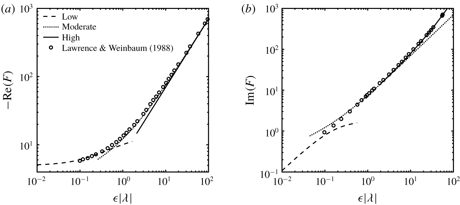
The force on a prolate spheroid of  $\unicode[STIX]{x1D716}=0.1$ undergoing longitudinal oscillations pertaining: (a) real part and (b) imaginary part.

Our asymptotic approximations for the real and imaginary parts of the force on a slender particle are plotted in figure 2 for a prolate spheroid of aspect ratio  $\unicode[STIX]{x1D716}=0.1$ and longitudinal profile
 $R(z)=(1-z^{2})^{1/2}$. Our results are in good agreement with the numerical computations via eigenfunction expansions in spheroidal coordinates of Lawrence & Weinbaum (Reference Lawrence and Weinbaum1988), which were digitized from their figure 2. Here, we reiterate that the low-frequency expansion (2.15) has an error that is logarithmic in
 $\unicode[STIX]{x1D716}$, while the moderate-frequency expansion (2.28) has an error that is algebraic in
 $\unicode[STIX]{x1D716}$; a huge difference in accuracy. Our approximations to the force in the three regimes allow for calculating the force over a larger range of
 $\unicode[STIX]{x1D716}|\unicode[STIX]{x1D706}|$ where it may be difficult to obtain numerical results using their eigenfunction expansion method. In addition, our asymptotic results are not restricted to a spheroid; they are valid for a general longitudinal profile, provided that
 $R(z)$ vanishes at the ends of the body and varies on the length scale of the particle.
3 Unsteady force for transverse oscillation
The axisymmetric, slender particle is now analysed while undergoing transverse oscillation in the  $x$-direction (figure 1b). We denote the velocity in the
 $x$-direction as
 $\hat{u}$.
3.1 Low-frequency transverse oscillation
A similar analysis to the longitudinal case is performed. The flow is quasi-steady on the scale of the inner region, where the velocity field is (Batchelor Reference Batchelor1970)
 $$\begin{eqnarray}\hat{u} =\frac{f(z;\unicode[STIX]{x1D716})}{4\unicode[STIX]{x03C0}}\left[\ln \left(\frac{\unicode[STIX]{x1D70C}}{R(z)}\right)-\frac{1}{2}\right]+1,\end{eqnarray}$$
where  $f(z;\unicode[STIX]{x1D716})$ is the dimensionless force per unit length in the
 $x$-direction on the particle. Since the particle is axisymmetric, the force is only in the
 $x$-direction. We rewrite (3.1) in terms of the outer coordinate
 $r$, as
 $$\begin{eqnarray}\hat{u} =\frac{f(z;\unicode[STIX]{x1D716})}{4\unicode[STIX]{x03C0}}\left[\ln \left(\frac{r}{R(z)}\right)+\ln \left(\frac{1}{\unicode[STIX]{x1D716}}\right)-\frac{1}{2}\right]+1,\end{eqnarray}$$
which suggests that  $f(z;\unicode[STIX]{x1D716})=O[1/\text{ln}(1/\unicode[STIX]{x1D716})]$ to leading order to ensure that the outer flow is bounded as
 $\unicode[STIX]{x1D716}\rightarrow 0$. The leading-order force per unit length
 $f(z;\unicode[STIX]{x1D716})=-4\unicode[STIX]{x03C0}/\text{ln}(1/\unicode[STIX]{x1D716})$, with the coefficient chosen to ensure the flow in the outer region is asymptotically small in
 $\unicode[STIX]{x1D716}$. This is twice the leading-order longitudinal force per unit length. We again pose a logarithmic expansion of
 $f(z;\unicode[STIX]{x1D716})$:
 $$\begin{eqnarray}f(z;\unicode[STIX]{x1D716})=-\frac{4\unicode[STIX]{x03C0}}{\ln (1/\unicode[STIX]{x1D716})}+\frac{f_{2}(z)}{\ln ^{2}(1/\unicode[STIX]{x1D716})}+O\left[\frac{1}{\ln ^{3}(1/\unicode[STIX]{x1D716})}\right].\end{eqnarray}$$
Combining (3.2) and (3.3) yields
 $$\begin{eqnarray}\hat{u} =-\frac{\ln (r)}{\ln (1/\unicode[STIX]{x1D716})}+\frac{1}{\ln (1/\unicode[STIX]{x1D716})}\left[\ln (R(z))+\frac{1}{2}+\frac{f_{2}}{4\unicode[STIX]{x03C0}}\right]+O\left[\frac{1}{\ln ^{2}(1/\unicode[STIX]{x1D716})}\right].\end{eqnarray}$$
Again, the outer velocity and pressure fields are expanded as
 $$\begin{eqnarray}\hat{\boldsymbol{v}}=\frac{\hat{\boldsymbol{v}}_{1}}{\ln (1/\unicode[STIX]{x1D716})}+O\left[\frac{1}{\ln ^{2}(1/\unicode[STIX]{x1D716})}\right]\quad \text{and}\quad \hat{p}=\frac{\hat{p}_{1}}{\ln (1/\unicode[STIX]{x1D716})}+O\left[\frac{1}{\ln ^{2}(1/\unicode[STIX]{x1D716})}\right],\end{eqnarray}$$
where  $\hat{\boldsymbol{v}}_{1}$ is the flow generated by a line distribution of oscillating Stokeslets, this time directed along
 $\boldsymbol{e}_{x}$; namely,
 $$\begin{eqnarray}\hat{\boldsymbol{v}}_{1}=\frac{1}{8\unicode[STIX]{x03C0}}\int _{-1}^{1}\boldsymbol{G}(\boldsymbol{x},\boldsymbol{x}_{0})\boldsymbol{\cdot }\left[h(z_{0})\boldsymbol{e}_{x}\right]\text{d}z_{0}.\end{eqnarray}$$
The outer velocity field component along  $\boldsymbol{e}_{x}$ is thus
 $$\begin{eqnarray}\hat{u} _{1}=\frac{1}{8\unicode[STIX]{x03C0}}\int _{-1}^{1}\left[\frac{Ah(z_{0})}{[r^{2}+(z-z_{0})^{2}]^{1/2}}+\frac{x^{2}Bh(z_{o})}{[r^{2}+(z-z_{0})^{2}]^{3/2}}\right]\text{d}z_{0}.\end{eqnarray}$$
The process for taking the limit of (3.7) as  $r\rightarrow 0$ is the same as that used for (2.12). Thus, as
 $r\rightarrow 0$ we have
 $$\begin{eqnarray}\hat{u} _{1}=\frac{h(z)}{4\unicode[STIX]{x03C0}}\left[\ln \left(\frac{2(1-z^{2})^{1/2}}{r}\right)+1\right]+\frac{1}{8\unicode[STIX]{x03C0}}\int _{-1}^{1}\frac{Ah(z_{0})-h(z)}{|z-z_{0}|}\,\text{d}z_{0}+o(1),\end{eqnarray}$$
where in (3.8)  $A$ has the argument
 $\unicode[STIX]{x1D706}|z-z_{0}|$. Matching (3.4) and (3.8) first yields a uniform source density
 $h(z)=4\unicode[STIX]{x03C0}$, which is twice that of the longitudinal case. Second, matching gives the
 $O[\ln ^{-2}(1/\unicode[STIX]{x1D716})]$ correction to the force per unit length,
 $f_{2}$, as
 $$\begin{eqnarray}\frac{f_{2}}{4\unicode[STIX]{x03C0}}=\ln \left[\frac{2(1-z^{2})^{1/2}}{R(z)}\right]+\frac{1}{2}+\frac{1}{2}\int _{-1}^{1}\frac{A-1}{|z-z_{0}|}\,\text{d}z_{0}.\end{eqnarray}$$
Upon integrating over the length of the particle, the total force is
 $$\begin{eqnarray}F_{L}=-\frac{8\unicode[STIX]{x03C0}}{\ln (1/\unicode[STIX]{x1D716})}+\frac{F_{2}}{\ln ^{2}(1/\unicode[STIX]{x1D716})}+O\left[\frac{1}{\ln ^{3}(1/\unicode[STIX]{x1D716})}\right],\end{eqnarray}$$
where
 $$\begin{eqnarray}\displaystyle F_{2} & = & \displaystyle 4\unicode[STIX]{x03C0}\int _{-1}^{1}\left[\ln \left[\frac{2(1-z^{2})^{1/2}}{R(z)}\right]+\frac{1}{2}\right]\text{d}z\nonumber\\ \displaystyle & & \displaystyle +\,2\unicode[STIX]{x03C0}\left[-2-4\unicode[STIX]{x1D6FE}+4(1-\ln (2\unicode[STIX]{x1D706}))-\left(\frac{1-2\unicode[STIX]{x1D706}-\text{e}^{-2\unicode[STIX]{x1D706}}}{\unicode[STIX]{x1D706}^{2}}\right)-\frac{2}{\unicode[STIX]{x1D706}}(\text{e}^{-2\unicode[STIX]{x1D706}}-1)-4E_{1}(2\unicode[STIX]{x1D706})\right].\nonumber\\ \displaystyle & & \displaystyle\end{eqnarray}$$
The low-frequency limit of (3.11) is
 $$\begin{eqnarray}\frac{F_{2}}{8\unicode[STIX]{x03C0}}=\frac{1}{2}\int _{-1}^{1}\left[\ln \left[\frac{2(1-z^{2})^{1/2}}{R(z)}\right]+\frac{1}{2}\right]\text{d}z-\frac{4}{3}\unicode[STIX]{x1D706}+O(\unicode[STIX]{x1D706}^{2}).\end{eqnarray}$$
From (2.18) and (2.19), taking  $\hat{\boldsymbol{U}}=\boldsymbol{e}_{x}$ in (2.18), the low-frequency expansion for the force on a slender particle moving transversely is
 $$\begin{eqnarray}\boldsymbol{F}=-\frac{8\unicode[STIX]{x03C0}}{\ln (1/\unicode[STIX]{x1D716})}\left[1+\frac{4\unicode[STIX]{x1D706}}{3\ln (1/\unicode[STIX]{x1D716})}\right]\boldsymbol{e}_{x}+O(\unicode[STIX]{x1D706}^{2}),\end{eqnarray}$$
whence it is seen that the  $O(\unicode[STIX]{x1D706})$ terms in (3.12) and (3.13) are equal.
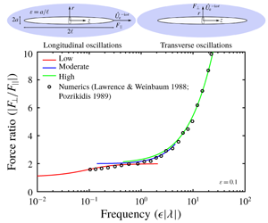
The ratio of the magnitude of the transverse force, say  $F_{\bot }$, to the longitudinal force, say
 $F_{\Vert }$, at low frequencies is from (2.15) and (3.10):
 $$\begin{eqnarray}\frac{F_{\bot }}{F_{\Vert }}=2+O\left[\frac{1}{\ln (1/\unicode[STIX]{x1D716})}\right].\end{eqnarray}$$
The leading factor of  $2$ recovers the well-known quasi-steady Stokes result that a slender particle experiences twice the force when undergoing transverse translation compared to longitudinal translation. Here, we have shown that (3.14) is also valid in unsteady Stokes flow, provided that
 $\unicode[STIX]{x1D716}|\unicode[STIX]{x1D706}|\ll 1$. Since
 $\unicode[STIX]{x1D716}\ll 1$, this does not require
 $|\unicode[STIX]{x1D706}|$ to be small; indeed
 $|\unicode[STIX]{x1D706}|$ could take on
 $O(1)$ values, such that unsteady effects are not small over the length of the slender particle.
The correction term in (3.10) again becomes comparable to the leading-order term when  $\unicode[STIX]{x1D716}|\unicode[STIX]{x1D706}|=O(1)$. Similar to the longitudinal case, at such ‘moderate’ frequency we cannot neglect unsteadiness in the inner region. This prompts a new asymptotic approximation in a moderate-frequency regime.
3.2 Moderate-frequency transverse oscillation
The flow in the inner region around a slender particle executing transverse oscillation at frequency  $\unicode[STIX]{x1D716}|\unicode[STIX]{x1D706}|=O(1)$ is approximately two-dimensional in the plane of the cross-section. The flow in the outer region is negligible, thus, at each section (in
 $z$) the velocity and pressure fields are given by those due to an infinite cylinder oscillating in the
 $x$-direction in unsteady Stokes flow, which is analysed by Holtzmark et al. (Reference Holtzmark, Johnsen, Sikkeland and Skavlem1954). The velocity field can be written in plane polar coordinates as
 $\unicode[STIX]{x1D6FC}\boldsymbol{e}_{r}+\unicode[STIX]{x1D6FD}\boldsymbol{e}_{\unicode[STIX]{x1D703}}$, where
 $\boldsymbol{e}_{r}$ and
 $\boldsymbol{e}_{\unicode[STIX]{x1D703}}$ are radial and polar unit vectors in the plane of the particle’s cross-section (figure 2b). Specifically, we have
 $\unicode[STIX]{x1D6FC}$,
 $\unicode[STIX]{x1D6FD}$, and pressure,
 $\hat{p}$, given by
 $$\begin{eqnarray}\displaystyle & \displaystyle \unicode[STIX]{x1D6FC}=-\cos \unicode[STIX]{x1D703}\left(\frac{R(z)^{2}}{\unicode[STIX]{x1D70C}^{2}}C-X-Z\right), & \displaystyle\end{eqnarray}$$
 $$\begin{eqnarray}\displaystyle & \displaystyle \unicode[STIX]{x1D6FD}=\sin \unicode[STIX]{x1D703}\left(-\frac{R(z)^{2}}{\unicode[STIX]{x1D70C}^{2}}C-X+Z\right), & \displaystyle\end{eqnarray}$$
 $$\begin{eqnarray}\displaystyle & \displaystyle \hat{p}=-\cos \unicode[STIX]{x1D703}\left(\frac{\unicode[STIX]{x1D716}\unicode[STIX]{x1D706}^{2}R(z)^{2}}{\unicode[STIX]{x1D70C}}C\right), & \displaystyle\end{eqnarray}$$
 $C$,
 $X$ and
 $Z$ are functions of frequency, cross-section shape and distance from the particle. In our notation, they are
 $$\begin{eqnarray}X=\frac{K_{0}(\unicode[STIX]{x1D716}\unicode[STIX]{x1D706}\unicode[STIX]{x1D70C})}{K_{0}(\unicode[STIX]{x1D716}\unicode[STIX]{x1D706}R(z))},\quad Z=-\frac{K_{2}(\unicode[STIX]{x1D716}\unicode[STIX]{x1D706}\unicode[STIX]{x1D70C})}{K_{0}(\unicode[STIX]{x1D716}\unicode[STIX]{x1D706}R(z))},\quad \text{and}\quad C=-\frac{K_{2}(\unicode[STIX]{x1D716}\unicode[STIX]{x1D706}R(z))}{K_{0}(\unicode[STIX]{x1D716}\unicode[STIX]{x1D706}R(z))}.\end{eqnarray}$$
The  $x$-component of the traction at the particle surface is
 $$\begin{eqnarray}\boldsymbol{e}_{x}\boldsymbol{\cdot }\unicode[STIX]{x1D748}\boldsymbol{\cdot }\boldsymbol{n}=\left[-\hat{p}+\frac{2}{\unicode[STIX]{x1D716}}\frac{\unicode[STIX]{x2202}\unicode[STIX]{x1D6FC}}{\unicode[STIX]{x2202}\unicode[STIX]{x1D70C}}\right]\cos \unicode[STIX]{x1D703}-\frac{1}{\unicode[STIX]{x1D716}}\left[\unicode[STIX]{x1D70C}\frac{\unicode[STIX]{x2202}}{\unicode[STIX]{x2202}\unicode[STIX]{x1D70C}}\left(\frac{\unicode[STIX]{x1D6FD}}{\unicode[STIX]{x1D70C}}\right)+\frac{1}{\unicode[STIX]{x1D70C}}\frac{\unicode[STIX]{x2202}\unicode[STIX]{x1D6FC}}{\unicode[STIX]{x2202}\unicode[STIX]{x1D703}}\right]\sin \unicode[STIX]{x1D703}+o(1).\end{eqnarray}$$
The force per unit length in the  $x$-direction is
 $f=\int _{0}^{2\unicode[STIX]{x03C0}}\unicode[STIX]{x1D716}R(z)(\boldsymbol{e}_{x}\boldsymbol{\cdot }\unicode[STIX]{x1D748}\boldsymbol{\cdot }\boldsymbol{n})\,\text{d}\unicode[STIX]{x1D703}$. Using (3.17) yields
 $$\begin{eqnarray}f=\unicode[STIX]{x03C0}\unicode[STIX]{x1D716}^{2}\unicode[STIX]{x1D706}^{2}R(z)^{2}C-\frac{2\unicode[STIX]{x03C0}\unicode[STIX]{x1D716}\unicode[STIX]{x1D706}R(z)K_{1}(\unicode[STIX]{x1D716}\unicode[STIX]{x1D706}R(z))}{K_{0}(\unicode[STIX]{x1D716}\unicode[STIX]{x1D706}R(z))},\end{eqnarray}$$
where the first term is the contribution of the normal stresses and the second term is the contribution of the tangential stresses. Using the identity  $K_{2}(\unicode[STIX]{x1D716}\unicode[STIX]{x1D706}R(z))=K_{0}(\unicode[STIX]{x1D716}\unicode[STIX]{x1D706}R(z))+[2/(\unicode[STIX]{x1D716}\unicode[STIX]{x1D706}R(z))]K_{1}(\unicode[STIX]{x1D716}\unicode[STIX]{x1D706}R(z))$, equation (3.18) simplifies to
 $$\begin{eqnarray}f=-\unicode[STIX]{x03C0}\unicode[STIX]{x1D716}^{2}\unicode[STIX]{x1D706}^{2}R(z)^{2}-4\unicode[STIX]{x03C0}\unicode[STIX]{x1D716}\unicode[STIX]{x1D706}R(z)\frac{K_{1}(\unicode[STIX]{x1D716}\unicode[STIX]{x1D706}R(z))}{K_{0}(\unicode[STIX]{x1D716}\unicode[STIX]{x1D706}R(z))},\end{eqnarray}$$
and the total force is thus
 $$\begin{eqnarray}F_{M}=-\unicode[STIX]{x03C0}\unicode[STIX]{x1D716}^{2}\unicode[STIX]{x1D706}^{2}\int _{-1}^{1}R(z)^{2}\,\text{d}z-4\unicode[STIX]{x03C0}\unicode[STIX]{x1D716}\unicode[STIX]{x1D706}\int _{-1}^{1}\frac{R(z)K_{1}(\unicode[STIX]{x1D716}\unicode[STIX]{x1D706}R(z))}{K_{0}(\unicode[STIX]{x1D716}\unicode[STIX]{x1D706}R(z))}\;\,\text{d}z.\end{eqnarray}$$
The first term in (3.20) is proportional to  $\unicode[STIX]{x1D706}^{2}$ and thus represents the inviscid acceleration reaction, which affects the force to leading order in the moderate-frequency regime for transverse translation, unlike the longitudinal case (see (2.28)). Recall, the acceleration reaction arises from the inviscid contribution to the pressure. The pressure makes a leading-order contribution to the traction (3.18) for moderate-frequency transverse oscillation, whereas it is subdominant for moderate-frequency longitudinal oscillation (2.28). Therefore, the acceleration reaction enters at leading order for moderate-frequency transverse oscillation, but not for longitudinal oscillation.
At moderate frequency, the force ratio from (2.28) and (3.20):
 $$\begin{eqnarray}\frac{F_{\bot }}{F_{\Vert }}=2+\frac{1}{2}\unicode[STIX]{x1D716}\unicode[STIX]{x1D706}\frac{\int _{-1}^{1}R(z)^{2}\,\text{d}z}{\int _{-1}^{1}R(z){\displaystyle \frac{K_{1}(\unicode[STIX]{x1D716}\unicode[STIX]{x1D706}R(z))}{K_{0}(\unicode[STIX]{x1D716}\unicode[STIX]{x1D706}R(z))}}\,\text{d}z},\end{eqnarray}$$
which can be greater than two by an  $O(1)$ amount since
 $\unicode[STIX]{x1D716}|\unicode[STIX]{x1D706}|=O(1)$. The increase in this ratio relative to the low frequency regime (see (3.14)) is due to leading-order effect of the acceleration reaction for moderate-frequency transverse oscillation.
3.3 High-frequency transverse oscillation
For  $\unicode[STIX]{x1D716}|\unicode[STIX]{x1D706}|\gg 1$, equation (3.20) reduces to
 $$\begin{eqnarray}F_{H}=-\unicode[STIX]{x1D716}\unicode[STIX]{x1D706}\int _{-1}^{1}4\unicode[STIX]{x03C0}R(z)\,\text{d}z-\unicode[STIX]{x03C0}\unicode[STIX]{x1D716}^{2}\unicode[STIX]{x1D706}^{2}\int _{-1}^{1}R(z)^{2}\,\text{d}z,\end{eqnarray}$$
where the factor of two difference between the terms proportional to  $\unicode[STIX]{x1D706}$ in (3.22) and (2.29) is consistent with the calculation of the Basset tensor, i.e. the coefficient of the high-frequency force proportional to
 $\unicode[STIX]{x1D706}$, in table 1 of Loewenberg (Reference Loewenberg1993) for high aspect ratio cylinders and spheroids. The subscript
 $H$ again stands for high frequency, although it should be understood this is not a distinguished limit as identified in § 2.3. Rather, equation (3.22) is simply the limiting form of (3.20) for
 $\unicode[STIX]{x1D716}|\unicode[STIX]{x1D706}|\gg 1$.
The force due to acceleration reaction in (3.22) is simply  $\unicode[STIX]{x1D706}^{2}$ multiplied by the (dimensionless) volume of the slender particle, normalized by
 $\ell ^{3}$. Thus, for a spheroid, of profile
 $R(z)=(1-z^{2})^{1/2}$, the high-frequency force is
 $$\begin{eqnarray}F_{H}|_{spheroid}=-2\unicode[STIX]{x03C0}^{2}\unicode[STIX]{x1D716}\unicode[STIX]{x1D706}-{\textstyle \frac{4}{3}}\unicode[STIX]{x03C0}\unicode[STIX]{x1D716}^{2}\unicode[STIX]{x1D706}^{2}.\end{eqnarray}$$
For a cylinder of profile  $R(z)=1$, the high-frequency force is
 $$\begin{eqnarray}F_{H}|_{cylinder}=-8\unicode[STIX]{x03C0}\unicode[STIX]{x1D716}\unicode[STIX]{x1D706}-2\unicode[STIX]{x03C0}\unicode[STIX]{x1D716}^{2}\unicode[STIX]{x1D706}^{2}.\end{eqnarray}$$
Note that (3.23) and (3.24) agree with the predictions from table 1 in Loewenberg (Reference Loewenberg1993).
Geer (Reference Geer1975) has analysed the transverse potential flow past a slender body. In particular, his equation (4.4) gives the (dimensionless) added mass under transverse motion as (in our notation)
 $$\begin{eqnarray}m_{a}^{\bot }=-\unicode[STIX]{x03C0}\unicode[STIX]{x1D716}^{2}\int _{-1}^{1}R(z)^{2}\,\text{d}z+O(\unicode[STIX]{x1D716}^{4}\ln \unicode[STIX]{x1D716}),\end{eqnarray}$$
which matches (3.22) from our analysis. That is, to leading order, transverse added mass is simply the volume of the body. Here, the error term is significantly smaller than the leading-order added mass by a factor of  $\unicode[STIX]{x1D716}^{2}\ln \unicode[STIX]{x1D716}$. For a slender spheroid, the added mass calculated from (3.25) is
 $$\begin{eqnarray}m_{a}^{\bot }=-{\textstyle \frac{4}{3}}\unicode[STIX]{x03C0}\unicode[STIX]{x1D716}^{2}+O(\unicode[STIX]{x1D716}^{4}\ln \unicode[STIX]{x1D716}),\end{eqnarray}$$
which matches (3.23), to leading order.
At high frequency, the force ratio is from (2.30) and (3.23):
 $$\begin{eqnarray}\frac{F_{\bot }}{F_{\Vert }}=\frac{\frac{2}{3}\unicode[STIX]{x1D716}\unicode[STIX]{x1D706}\displaystyle \int _{-1}^{1}R(z)\,\text{d}z}{1-\frac{2}{3}\unicode[STIX]{x1D716}\unicode[STIX]{x1D706}\boldsymbol{\cdot }\unicode[STIX]{x1D716}^{2}\ln \unicode[STIX]{x1D716}\;\left(\displaystyle \int _{-1}^{1}R(z)\,\text{d}z\right)^{-1}}.\end{eqnarray}$$
Clearly, the ratio of the forces is very large, since  $\unicode[STIX]{x1D716}|\unicode[STIX]{x1D706}|\gg 1$ in the high-frequency regime. Physically, this occurs because the acceleration reaction is the dominant contribution to the force, and the transverse added mass is
 $O(\unicode[STIX]{x1D716}^{-2})$ larger than the longitudinal added mass for a particle with zero thickness at its ends. Evidently, at large frequency there is a huge difference in the forces for longitudinal versus transverse oscillation, purely due to inviscid effects. This difference only manifests in the imaginary part of the force, since the force due to the acceleration reaction is proportional to
 $\unicode[STIX]{x1D706}^{2}$: e.g. compare the magnitudes of
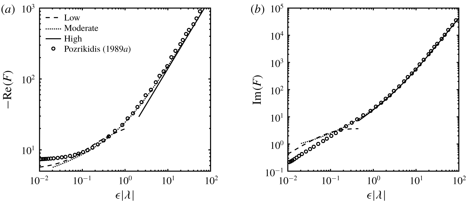
 $\text{Im}(F)$ in figures 2(b) and 3(b) for
 $\unicode[STIX]{x1D716}|\unicode[STIX]{x1D706}|>10$. In contrast,
 $\text{Re}(F)$ in figures 2(a) and 3(a) are of a comparable order of magnitude over the entire frequency range shown. Finally, note that at very large frequency,
 $\unicode[STIX]{x1D716}|\unicode[STIX]{x1D706}|\gg |\unicode[STIX]{x1D716}^{2}\ln \unicode[STIX]{x1D716}|^{-1}$ (note, this is beyond the range shown in figures 2 and 3), from (3.27) we have
 $F_{\bot }/F_{\Vert }\sim |\unicode[STIX]{x1D716}^{2}\ln \unicode[STIX]{x1D716}|^{-1}$ which is simply the ratio of the added masses and thus independent of the particle shape and frequency.
3.4 Transverse oscillation force results
The force on a prolate spheroid of  $\unicode[STIX]{x1D716}=0.1$ undergoing transverse oscillations pertaining: (a) real part and (b) imaginary part.

Our asymptotic approximations of the force for transverse oscillation are plotted in figure 3 for a prolate spheroid of  $\unicode[STIX]{x1D716}=0.1$. Our results are in good agreement with the boundary integral computations digitized from figure 4 of Pozrikidis (Reference Pozrikidis1989a). The greatest discrepancy is for
 $\unicode[STIX]{x1D716}|\unicode[STIX]{x1D706}|\ll 1$ due to
 $\unicode[STIX]{x1D716}=0.1$ only being moderately small, and our low-frequency expansion having errors logarithmic in
 $\unicode[STIX]{x1D716}$. We are confident that our expansion is correct since it matches with Lawrence & Weinbaum’s expression for the force on an arbitrary particle at low frequency, equation (3.13).
4 Conclusion
Asymptotic approximations were derived for the hydrodynamic force on a slender particle undergoing longitudinal or transverse oscillations in unsteady Stokes flow. Low, moderate and high oscillation frequency regimes were identified and examined in both cases. In the low-frequency regime,  $\unicode[STIX]{x1D716}\rightarrow 0$ and
 $\unicode[STIX]{x1D716}|\unicode[STIX]{x1D706}|\ll 1$, the period of oscillation is much longer than the vorticity diffusion time on the scale of the cross-sectional width of the particle, leading to quasi-steady Stokes flow in the inner region and unsteady Stokes flow in the outer region. As frequency increases to
 $\unicode[STIX]{x1D716}|\unicode[STIX]{x1D706}|=O(1)$ these two time scales become comparable leading to unsteady flow in the inner region. Here, the body shape has a leading-order effect on the force, unlike in the low-frequency regime. In the high-frequency regime the force consists of a history contribution proportional to
 $\unicode[STIX]{x1D706}$ and an acceleration reaction contribution proportional to
 $\unicode[STIX]{x1D706}^{2}$. The latter only affects the imaginary part of the force. We summarize our asymptotic approximations in table 1.
Summary of various asymptotic approximations to the force.

The present analysis can be used, in principle, to solve the initial-value problem when the particle is suddenly set into motion at  $t=0$, such that its velocity is
 $$\begin{eqnarray}\boldsymbol{U}(t)=\left\{\begin{array}{@{}ll@{}}0, & t<0,\\ \boldsymbol{U}, & t\geqslant 0.\end{array}\right.\end{eqnarray}$$
Note that the Laplace transform  ${\mathcal{L}}\{\boldsymbol{U}(t)\}=\boldsymbol{U}/s$, where
 $s$ is the Laplace frequency. We simply set
 $-\text{i}\unicode[STIX]{x1D714}\rightarrow s$ in our analysis to apply our results to this initial-value problem (Yang & Leal Reference Yang and Leal1991).
In general, the dependence of the force on frequency is too complicated to allow for an analytic inversion to the time domain. However, we can make progress for very low and high frequencies corresponding to long and short times, respectively. In the former case from (2.15) and (2.17) we have for longitudinal translation
 $$\begin{eqnarray}\displaystyle F_{L} & {\sim} & \displaystyle \frac{-4\unicode[STIX]{x03C0}}{\ln (1/\unicode[STIX]{x1D716})}+\frac{4\unicode[STIX]{x03C0}}{\ln ^{2}(1/\unicode[STIX]{x1D716})}\left\{\frac{1}{2}\int _{-1}^{1}\left[\ln \left[\frac{2(1-z^{2})^{1/2}}{R(z)}\right]-\frac{1}{2}\right]\text{d}z-\frac{2}{3}\unicode[STIX]{x1D706}+O(\unicode[STIX]{x1D706}^{2})\right\}\nonumber\\ \displaystyle & & \displaystyle +\,O\left[\frac{1}{\ln ^{3}(1/\unicode[STIX]{x1D716})}\right].\end{eqnarray}$$
Thus, the transformation  $-\text{i}\unicode[STIX]{x1D714}\rightarrow s$ gives
 $$\begin{eqnarray}F_{L}\sim \frac{1}{S}\left(\frac{-4\unicode[STIX]{x03C0}}{\ln (1/\unicode[STIX]{x1D716})}+\frac{4\unicode[STIX]{x03C0}}{\ln ^{2}(1/\unicode[STIX]{x1D716})}\left\{\frac{1}{2}\int _{-1}^{1}\left[\ln \left[\frac{2(1-z^{2})^{1/2}}{R(z)}\right]-\frac{1}{2}\right]\text{d}z-\frac{2}{3}S^{1/2}+O(S^{2})\right\}\right),\end{eqnarray}$$
where  $S=s\ell ^{2}/\unicode[STIX]{x1D708}$. Noting that
 ${\mathcal{L}}^{-1}(S^{-1/2})=T^{-1/2}/\sqrt{\unicode[STIX]{x03C0}}$ where
 $T=t\unicode[STIX]{x1D708}/\ell ^{2}$, we have
 $$\begin{eqnarray}F_{L}\sim \frac{-4\unicode[STIX]{x03C0}}{\ln (1/\unicode[STIX]{x1D716})}+\frac{2\unicode[STIX]{x03C0}}{\ln ^{2}(1/\unicode[STIX]{x1D716})}\left(\int _{-1}^{1}\left[\ln \left[\frac{2(1-z^{2})^{1/2}}{R(z)}\right]-\frac{1}{2}\right]\text{d}z\right)-\frac{8\sqrt{\unicode[STIX]{x03C0}}}{3\ln ^{2}(1/\unicode[STIX]{x1D716})}\frac{1}{T^{1/2}}+\cdots\end{eqnarray}$$
That is, the approach to the steady drag scales as  $T^{-1/2}$: this algebraic decay is known as a ‘long-time tail’, and the
 $-1/2$ power is characteristic of any object that exerts a net hydrodynamic force on the fluid.
At high frequency, transforming  $-\text{i}\unicode[STIX]{x1D714}\rightarrow s$ in (2.30) and inverting gives the short-time behaviour
 $$\begin{eqnarray}F_{H}=-\left(\unicode[STIX]{x1D716}\int _{-1}^{1}2\unicode[STIX]{x03C0}R(z)\,\text{d}z\right)\frac{1}{T^{1/2}}-2\unicode[STIX]{x03C0}\unicode[STIX]{x1D716}^{4}\ln \unicode[STIX]{x1D716}\left[\int _{-1}^{1}\left(R(z)\frac{\text{d}R(z)}{\text{d}z}\right)\text{d}z\right]\unicode[STIX]{x1D6FF}(T),\end{eqnarray}$$
where  $\unicode[STIX]{x1D6FF}(T)$ is the delta function and the first term shows a short-time decay of the force as
 $T^{-1/2}$; this decay is also seen for a flat plate (Lord Rayleigh Reference Rayleigh1911) and is the first approximation for an infinite cylinder of arbitrary cross-section (Batchelor Reference Batchelor1954). The second term is the acceleration reaction associated with the sudden motion at
 $T=0$. Even though the force diverges as
 $T\rightarrow 0$, the total impulse is integrable.
Similarly for transverse translation at low frequency, transforming  $-\text{i}\unicode[STIX]{x1D714}\rightarrow s$ in (3.10) and (3.12) and inverting gives the long-time behaviour
 $$\begin{eqnarray}F_{L}\sim \frac{-8\unicode[STIX]{x03C0}}{\ln (1/\unicode[STIX]{x1D716})}+\frac{4\unicode[STIX]{x03C0}}{\ln ^{2}(1/\unicode[STIX]{x1D716})}\left(\int _{-1}^{1}\left[\ln \left[\frac{2(1-z^{2})^{1/2}}{R(z)}\right]+\frac{1}{2}\right]\text{d}z\right)-\frac{32\sqrt{\unicode[STIX]{x03C0}}}{3\ln ^{2}(1/\unicode[STIX]{x1D716})}\frac{1}{T^{1/2}}+\cdots \,.\end{eqnarray}$$
For transverse translation at high frequency, transforming  $-\text{i}\unicode[STIX]{x1D714}\rightarrow s$ in (3.22) and inverting gives the short-time behaviour
 $$\begin{eqnarray}F_{H}=-\left(\unicode[STIX]{x1D716}\int _{-1}^{1}4\unicode[STIX]{x03C0}R(z)\,\text{d}z\right)\frac{1}{T^{1/2}}-\left(\unicode[STIX]{x1D716}^{2}\int _{-1}^{1}\unicode[STIX]{x03C0}R(z)^{2}\,\text{d}z\right)\unicode[STIX]{x1D6FF}(T).\end{eqnarray}$$
Acknowledgements
J.K.K. thanks the Air Products Graduate Fellowship and the Sharbaugh Presidential Fellowship for financial support.
Declaration of interests
The authors report no conflict of interest.