1 Introduction
The idea that turbulent fluid flow can be studied in terms of the invariant solutions of Navier–Stokes equations dates back to the 1940s (Hopf Reference Hopf1948). Examples of such invariant solutions (also called ‘exact coherent states’ or ‘recurrent flows’ in the fluid dynamics literature) are steady states (or equilibria), travelling waves (or relative equilibria), periodic orbits, relative periodic orbits and partially hyperbolic tori. A turbulent flow is then viewed as a walk from the neighbourhood of one invariant solution to the other. If all these solutions are unstable, the turbulent trajectory never settles down and its itinerary becomes desperately complex.
Initially a mathematical endeavour, this view has been put to practice over the last 15 years in many experimental and numerical studies, providing insights that are beyond the reach of purely statistical descriptions of turbulence – see Kawahara, Uhlmann & van Veen (Reference Kawahara, Uhlmann and van Veen2012) and Cvitanović (Reference Cvitanović2013), for reviews.
The invariant solutions of the Navier–Stokes equations often exhibit complex spatiotemporal behaviours, and hence analytic expressions for them are unavailable. Their numerical computation was first explored in the pioneering works of Marcus & Tuckerman (Reference Marcus and Tuckerman1987) and Nagata (Reference Nagata1990). Nagata found the first non-trivial equilibrium and travelling-wave solutions of the plane Couette flow (Nagata Reference Nagata1990, Reference Nagata1997). Nagata’s approach to finding these solutions is the following. Through a finite truncation, the invariant solutions are formulated as the zeros of a large system of nonlinear algebraic equations
 $\boldsymbol{F}(\boldsymbol{a})=\mathbf{0}$
. The solution
 $\boldsymbol{a}$
is then found through Newton–Raphson iterations. Depending on the type of the discretization, the finite vector
 $\boldsymbol{a}$
contains either the Galerkin coefficients or the collocation values.
Nagata’s approach underlies the state-of-the-art methods for finding invariant solutions of fluid flow (see e.g. Waleffe Reference Waleffe1998; Kawahara & Kida Reference Kawahara and Kida2001; Viswanath Reference Viswanath2007; Gibson, Halcrow & Cvitanović Reference Gibson, Halcrow and Cvitanović2009; Willis, Cvitanović & Avila Reference Willis, Cvitanović and Avila2013). Such Newton-type approaches suffer from two major drawbacks:
-
(i) Obtaining the Newton direction
 ${\it\delta}\boldsymbol{a}$
requires solving the linear system of equations
$\boldsymbol{{\rm\nabla}}\boldsymbol{F}(\boldsymbol{a}){\it\delta}\boldsymbol{a}=-\boldsymbol{F}(\boldsymbol{a})$
. Even for moderate Reynolds numbers, this linear equation is too large to be solved accurately (within numerical precision) in reasonable computation time.
-
(ii) The convergence of the Newton iterations is not generally guaranteed. The iterations converge only if very good initial guesses are provided.


As regards item (i), the linear system is typically too large for the matrix
 $\boldsymbol{{\rm\nabla}}\boldsymbol{F}(\boldsymbol{a})$
to be even explicitly formed (due to memory considerations). To address this issue, the generalized minimal residual (GMRES) method is used to approximate the solution of the linear system (Saad & Schultz Reference Saad and Schultz1986). The GMRES method replaces the exact Newton direction with its least-square approximation within a Krylov subspace. Forming this subspace only requires the action of the matrix
 $\boldsymbol{{\rm\nabla}}\boldsymbol{F}(\boldsymbol{a})$
on certain vectors, hence avoiding the formation of the matrix itself. The resulting method is often referred to as Newton–GMRES iterations. Although computationally feasible, Newton–GMRES iterations are still a formidable numerical undertaking in terms of implementation and computation time.
As mentioned in item (ii) above, even when the exact Newton descent direction
 ${\it\delta}\boldsymbol{a}$
is known, the iterations are not guaranteed to converge. Newton’s domain of convergence in the context of Navier–Stokes equations is typically small, demanding a very good initial guess for the iterations to converge (Waleffe Reference Waleffe1997). The Newton iterations, therefore, are very effective for bifurcation analysis where the invariant solutions bifurcate from known solutions (Tuckerman et al.
Reference Tuckerman, Bertagnolio, Daube, Quéré, Barkley, Henry and Bergeon2000; Waleffe Reference Waleffe2003; Kreilos & Eckhardt Reference Kreilos and Eckhardt2012). In this case, the known solution (corresponding to the old bifurcation parameter value) is used as the initial guess for the Newton iterations. Even then, the method might fail to determine solutions far from the bifurcation point.
In practice, good initial guesses for Newton iterations are obtained through heuristic methods, such as close recurrences of a turbulent trajectory (Auerbach et al. Reference Auerbach, Cvitanović, Eckmann, Gunaratne and Procaccia1987; Kawahara, Kida & Van Veen Reference Kawahara, Kida and Van Veen2006; Viswanath Reference Viswanath2007; Cvitanović & Gibson Reference Cvitanović and Gibson2010). Such heuristics lack a solid mathematical basis. As a result, many important invariant solutions may and will remain undiscovered (see § 5).
Viswanath (Reference Viswanath2007) used the hook step together with the Newton–GMRES method, which significantly improved the convergence of the iterations. The underlying idea of the hook step is to approximate the Newton direction within the Krylov subspace with the constraint that
 ${\it\delta}\boldsymbol{a}$
belongs to a ‘trust region’ such that
 $|{\it\delta}\boldsymbol{a}|$
is smaller than some prescribed value
 ${\it\epsilon}$
. The constraint
 $|{\it\delta}\boldsymbol{a}|<{\it\epsilon}$
ensures that the linearization
 $\boldsymbol{{\rm\nabla}}\boldsymbol{F}(\boldsymbol{a}){\it\delta}\boldsymbol{a}$
involved in Newton iterations is a valid approximation (Dennis & Schnabel Reference Dennis and Schnabel1996). The resulting method, i.e. the Newton–GMRES–hook iterations, is state of the art in computing invariant solutions in the context of fluid flow. While improving the convergence chance of the Newton–GMRES iterations, the hook step still requires a good initial guess.
Such drawbacks have slowed down research progress in transitional and moderate-Reynolds-number turbulence. As the study of fluid turbulence through its invariant solutions reaches a mature state, it is time to revisit the methods by which these invariant solutions are found. Better methods should ideally scale linearly (in the sense of computational complexity) with the number of degrees of freedom and be universally convergent. The term ‘universally convergent’ implies that every initial guess converges to some solution. Universally convergent methods, however, do not immediately guarantee the identification of all possible solutions from a finite set of initial guesses.
The main goal of the present paper is to propose one such new direction. We develop an adjoint-based method for computing steady-state and travelling-wave solutions of incompressible Navier–Stokes equations with periodic boundary conditions. In particular, adjoint partial differential equations (PDEs) are derived whose trajectories converge to (relative) equilibria of the Navier–Stokes equations.
Adjoint equations appear naturally in optimal control, where the governing equations act as constraints – see Gunzburger (Reference Gunzburger2002) for a survey of applications in fluid dynamics. Pringle & Kerswell (Reference Pringle and Kerswell2010) and Monokrousos et al. (Reference Monokrousos, Bottaro, Brandt, Di Vita and Henningson2011) used adjoint-based optimization to find the optimal route to turbulence in transitional shear flows – see also Kerswell, Pringle & Willis (Reference Kerswell, Pringle and Willis2014) for a review. To investigate the regularity of the Navier–Stokes equations, Ayala & Protas (Reference Ayala and Protas2014) use adjoint-based optimization to find the initial conditions that result in maximal palinstrophy growth.
To the best of our knowledge, adjoint-based methods have not been used to find invariant solutions of the Navier–Stokes equations. They have, however, been utilized in the context of nonlinear wave equations. For instance, Ambrose & Wilkening (Reference Ambrose and Wilkening2010b ) formulate the time-periodic solutions of a unidirectional water wave equation as the minima of an appropriate functional. The minima are found iteratively by a ‘steepest descent’ method. At each iteration, the descent direction is obtained as the solution of a backward-time adjoint PDE (see also Ambrose & Wilkening Reference Ambrose and Wilkening2010a ). Yang & Lakoba (Reference Yang and Lakoba2007) realized that, for equilibrium solutions, the descent direction can be expressed explicitly. Namely, they show that the solitary solutions of nonlinear wave equations coincide with the asymptotically stable equilibria of an adjoint PDE.
The case of Navier–Stokes equations is more involved due to the presence of non-local pressure gradients enforcing incompressibility. This calls for a special treatment as presented here. We also extend the adjoint-based approach to finding travelling-wave solutions with a priori unknown wave speeds.
Recently, Chandler & Kerswell (Reference Chandler and Kerswell2013) and Lucas & Kerswell (Reference Lucas and Kerswell2014) carried out the most exhaustive search for invariant solutions of a chaotic two-dimensional Kolmogorov flow using Newton–GMRES–hook iterations. Here, we apply our adjoint-based method to the same Kolmogorov flow and discover several new steady-state and travelling-wave solutions. We show that some of these new solutions underpin the temporal intermittencies associated with short-lived, rapid growth of energy dissipation.
This paper is organized as follows. The preliminary material is reviewed in § 2, in a rather general setting. The explicit form of the adjoint equations for Navier–Stokes equations are presented in § 3. We test the adjoint-based approach in § 4 on a two-dimensional Kolmogorov flow and also carry out a thorough comparison with Newton–GMRES–hook iterations. In § 5, the temporal intermittency of the Kolmogorov flow is studied in terms of its invariant solutions. Finally, § 6 contains our concluding remarks and an outline of future research directions.
2 Preliminaries: Newton descent versus adjoint descent
In this section, we review Newton and adjoint descent methods in a general framework. We find this exposition helpful for understanding the Navier–Stokes adjoint equations presented in § 3.
Consider the PDE
 $$\begin{eqnarray}\displaystyle \partial _{t}\boldsymbol{u}=\boldsymbol{F}(\boldsymbol{u}), & & \displaystyle\end{eqnarray}$$
where the real-valued vector field
 $\boldsymbol{u}(\boldsymbol{x},t)$
is a function of space
 $\boldsymbol{x}$
and time
 $t$
, and
 $\boldsymbol{F}$
is a nonlinear differential operator acting on an inner product function space
 $\mathscr{H}$
. We seek equilibrium (or steady-state) solutions of this PDE, i.e. time-independent vector fields
 $\boldsymbol{u}=\boldsymbol{u}(\boldsymbol{x})$
such that
 $\boldsymbol{F}(\boldsymbol{u})=\mathbf{0}$
.
The finite-dimensional counterpart of (2.1) is the system of ordinary differential equations (ODEs)
 $\text{d}\boldsymbol{a}/\text{d}t=\boldsymbol{F}(\boldsymbol{a})$
, where
 $\boldsymbol{a}\in \mathbb{R}^{d}$
and
 $\boldsymbol{F}:\mathbb{R}^{d}\rightarrow \mathbb{R}^{d}$
. While our derivations are in the infinite-dimensional setting, we will occasionally invoke this finite-dimensional analogue to elaborate the ideas.
We define the ‘weighted’ inner product
 $$\begin{eqnarray}\displaystyle \langle \boldsymbol{u},\boldsymbol{u}^{\prime }\rangle _{\mathscr{A}}=\langle \boldsymbol{u},\mathscr{A}\boldsymbol{u}^{\prime }\rangle _{L^{2}}, & & \displaystyle\end{eqnarray}$$
for any two functions
 $\boldsymbol{u},\boldsymbol{u}^{\prime }\in \mathscr{H}$
, where
 $\mathscr{A}$
denotes a real-valued, positive-definite, self-adjoint (with respect to the
 $L^{2}$
inner product
 $\langle \cdot ,\cdot \rangle _{L^{2}}$
) operator. The prime signs should not be confused with derivatives; we use them here to distinguish different functions. The inner product (2.2) defines a natural norm given by
 $$\begin{eqnarray}\displaystyle \Vert \boldsymbol{u}\Vert _{\mathscr{A}}=\sqrt{\langle \boldsymbol{u},\boldsymbol{ u}\rangle _{\mathscr{A}}}, & & \displaystyle\end{eqnarray}$$
for
 $\boldsymbol{u}\in \mathscr{H}$
. The choice of
 $\mathscr{A}$
is somewhat arbitrary and should be judiciously chosen for a specific problem. For the Navier–Stokes equation, for instance, we will use an operator that is closely related to the inverse of the Laplacian (see § 3). For this exposition, however, we set
 $\mathscr{A}$
to the identity, which renders (2.2) as the usual
 $L^{2}$
inner product.
With this setting, we seek a second PDE
 $$\begin{eqnarray}\displaystyle \partial _{{\it\tau}}\boldsymbol{u}=\boldsymbol{G}(\boldsymbol{u}), & & \displaystyle\end{eqnarray}$$
such that its solutions converge to the equilibrium solutions of (2.1) as the fictitious time
 ${\it\tau}$
tends to infinity. To ensure this convergence, the differential operator
 $\boldsymbol{G}$
is designed in a specific way such that
 $$\begin{eqnarray}\displaystyle \Vert \boldsymbol{F}(\boldsymbol{u}({\it\tau}))\Vert _{L^{2}}\rightarrow 0,\quad \text{as }{\it\tau}\rightarrow \infty , & & \displaystyle\end{eqnarray}$$
where
 $\boldsymbol{u}({\it\tau})=\boldsymbol{u}(\cdot ,{\it\tau})$
denotes a solution of (2.4). Newton and adjoint descents correspond to two different choices of the operator
 $\boldsymbol{G}$
.
The finite-dimensional analogue of (2.4) is the fictitious-time ODE
 $\text{d}\boldsymbol{a}/\text{d}{\it\tau}=\boldsymbol{G}(\boldsymbol{a})$
with
 $\boldsymbol{G}:\mathbb{R}^{d}\rightarrow \mathbb{R}^{d}$
.
2.1 Newton descent
The main observation here is that discrete Newton iterations are an explicit Euler approximation of a continuous fictitious-time dynamical system (Saupe Reference Saupe1988). This well-known fact is rarely mentioned in the literature, prompting Smale (Reference Smale1981) to write ‘This geometry is based on an idea which is known, but not usually explicated. Namely, Newton’s method for solving
 $f(z)=0$
is an Euler approximation to the ordinary differential equation …’. Here, we first derive the continuous fictitious-time Newton method in the infinite-dimensional setting and then show how the discrete Newton iterations follow from there.
The norm
 $\Vert \boldsymbol{F}(\boldsymbol{u})\Vert _{L^{2}}$
evolves along the trajectories of (2.4) according to
 $$\begin{eqnarray}\displaystyle \partial _{{\it\tau}}\Vert \boldsymbol{F}(\boldsymbol{u})\Vert _{L^{2}}^{2}=2\langle \mathbf{\mathscr{L}}(\boldsymbol{u};\boldsymbol{G}(\boldsymbol{u})),\boldsymbol{F}(\boldsymbol{u})\rangle _{L^{2}}, & & \displaystyle\end{eqnarray}$$
where the linear operator
 $\mathbf{\mathscr{L}}(\boldsymbol{u};\cdot )$
is the Gâteaux derivative of
 $\boldsymbol{F}$
evaluated at the state
 $\boldsymbol{u}$
, and is defined by
 $$\begin{eqnarray}\displaystyle \mathbf{\mathscr{L}}(\boldsymbol{u};\boldsymbol{u}^{\prime }):=\lim _{{\it\epsilon}\rightarrow 0}\frac{\boldsymbol{F}(\boldsymbol{u}+{\it\epsilon}\boldsymbol{u}^{\prime })-\boldsymbol{F}(\boldsymbol{u})}{{\it\epsilon}},\quad \forall \boldsymbol{u}^{\prime }\in \mathscr{H}. & & \displaystyle\end{eqnarray}$$
Requiring
 $\boldsymbol{G}$
to satisfy
 $$\begin{eqnarray}\displaystyle \mathbf{\mathscr{L}}(\boldsymbol{u};\boldsymbol{G}(\boldsymbol{u}))=-\boldsymbol{F}(\boldsymbol{u}), & & \displaystyle\end{eqnarray}$$
one obtains the continuous fictitious-time Newton descent in infinite dimensions. Substituting this expression in (2.6), we obtain
 $$\begin{eqnarray}\displaystyle \partial _{{\it\tau}}\Vert \boldsymbol{F}(\boldsymbol{u}({\it\tau}))\Vert _{L^{2}}^{2}=-2\Vert \boldsymbol{F}(\boldsymbol{u}({\it\tau}))\Vert _{L^{2}}^{2}, & & \displaystyle\end{eqnarray}$$
which has the exact solution
 $\Vert \boldsymbol{F}(\boldsymbol{u}({\it\tau}))\Vert _{L^{2}}=\Vert \boldsymbol{F}(\boldsymbol{u}(0))\Vert _{L^{2}}\exp (-{\it\tau})$
. This shows that, as long as (2.8) has a solution,
 $\Vert \boldsymbol{F}(\boldsymbol{u}({\it\tau}))\Vert _{L^{2}}$
decays to zero exponentially fast along the solutions of (2.4). In other words, the continuous fictitious-time Newton method converges to an equilibrium solution of (2.1) for almost all initial conditions (Saupe Reference Saupe1988; Cvitanović & Lan Reference Cvitanović, Lan and Antoniou2003; Lan & Cvitanović Reference Lan and Cvitanović2004).
For a given state
 $\boldsymbol{u}$
, (2.8) is a PDE that can in principle be solved for
 $\boldsymbol{G}$
. In practice, it is approximated through some finite truncation to take the form
 $\boldsymbol{{\rm\nabla}}\boldsymbol{F}(\boldsymbol{a})\boldsymbol{G}(\boldsymbol{a})=-\boldsymbol{F}(\boldsymbol{a})$
, with
 $\boldsymbol{a}$
being the Galerkin coefficients. The solution
 $\boldsymbol{G}$
of this large, but finite-dimensional, linear system is often approximated by some variant of GMRES iterations (Trefethen & Bau Reference Trefethen and Bau1997).
Furthermore, the PDE (2.4) is discretized in time to yield the explicit Euler step
 $$\begin{eqnarray}\boldsymbol{u}_{i+1}=\boldsymbol{u}_{i}+{\it\delta}{\it\tau}\boldsymbol{G}(\boldsymbol{u}_{i}),\end{eqnarray}$$
with
 $0<{\it\delta}{\it\tau}\leqslant 1$
. The standard Newton iterations correspond to
 ${\it\delta}{\it\tau}=1$
, while damped Newton iterations adjust
 ${\it\delta}{\it\tau}$
in order to ensure that the
 $L^{2}$
norm decreases (Boyd & Vandenberghe Reference Boyd and Vandenberghe2004).
The above discrete iterations do not guarantee the global convergence that the continuous fictitious-time Newton descent does (Saupe Reference Saupe1988). As mentioned in the introduction, the convergence of Newton iterations is only guaranteed if the initial guess is sufficiently close to an equilibrium. In fact, if such a close initial guess is available, the convergence to the equilibrium is super-exponential (Deuflhard Reference Deuflhard2011).
Anecdotal evidence suggests that, in the context of fluid flow, the basin of attraction of Newton iterations is rather small (Waleffe Reference Waleffe1997; Viswanath Reference Viswanath2007). This domain can be enlarged by choosing a higher-order scheme for temporal discretization of (2.4). This is, however, computationally too demanding for large-dimensional systems, such as turbulent fluid flow.
2.2 Adjoint descent
The adjoint descent corresponds to an alternative choice of
 $\boldsymbol{G}$
that may be expressed analytically, thus avoiding the approximation involved in the Newton–GMRES iterations. Moreover, the adjoint direction can be evaluated at a relatively low computational cost, rendering a higher-order time discretization of (2.4) feasible.
To express the adjoint direction, note that (2.6) can be written as
 $$\begin{eqnarray}\displaystyle \partial _{{\it\tau}}\Vert \boldsymbol{F}(\boldsymbol{u})\Vert _{L^{2}}^{2}=2\langle \boldsymbol{G}(\boldsymbol{u}),\mathbf{\mathscr{L}}^{\dagger }(\boldsymbol{u};\boldsymbol{F}(\boldsymbol{u}))\rangle _{L^{2}}, & & \displaystyle\end{eqnarray}$$
where the adjoint
 $\mathbf{\mathscr{L}}^{\dagger }(\boldsymbol{u};\cdot )$
is the linear operator satisfying
 $$\begin{eqnarray}\displaystyle \langle \mathbf{\mathscr{L}}(\boldsymbol{u};\boldsymbol{u}^{\prime }),\boldsymbol{u}^{\prime \prime }\rangle _{L^{2}}=\langle \boldsymbol{u}^{\prime },\mathbf{\mathscr{L}}^{\dagger }(\boldsymbol{u};\boldsymbol{u}^{\prime \prime })\rangle _{L^{2}},\quad \forall \boldsymbol{u},\boldsymbol{u}^{\prime },\boldsymbol{u}^{\prime \prime }\in L^{2}. & & \displaystyle\end{eqnarray}$$
Requiring
 $$\begin{eqnarray}\displaystyle \boldsymbol{G}(\boldsymbol{u})=-\mathbf{\mathscr{L}}^{\dagger }(\boldsymbol{u};\boldsymbol{F}(\boldsymbol{u})) & & \displaystyle\end{eqnarray}$$
ensures the descent of the norm
 $\Vert \boldsymbol{F}(\boldsymbol{u}({\it\tau}))\Vert _{L^{2}}$
along the trajectories of (2.4), since
 $$\begin{eqnarray}\displaystyle \partial _{{\it\tau}}\Vert \boldsymbol{F}(\boldsymbol{u})\Vert _{L^{2}}^{2}=-2\Vert \mathbf{\mathscr{L}}^{\dagger }(\boldsymbol{u};\boldsymbol{F}(\boldsymbol{u}))\Vert _{L^{2}}^{2}\leqslant 0. & & \displaystyle\end{eqnarray}$$
We refer to
 $\boldsymbol{G}$
given by (2.13) as the adjoint direction. The finite-dimensional analogue of this adjoint direction is
 $\boldsymbol{G}(\boldsymbol{a})=-[\boldsymbol{{\rm\nabla}}\boldsymbol{F}(\boldsymbol{a})]^{\text{T}}\boldsymbol{F}(\boldsymbol{a})$
, where
 $\text{T}$
denotes the usual matrix transposition.
The downside of using the adjoint descent is that, unlike the continuous fictitious-time Newton descent, (2.14) does not guarantee an exponential decay of the
 $L^{2}$
norm. In fact, we observe a relatively slow decay in § 4.3, and propose a hybrid adjoint–Newton algorithm to rectify this drawback.
In § 3, we derive the explicit form of the adjoint operator for the incompressible Navier–Stokes equations.
3 Adjoint descent for the Navier–Stokes equations
Consider the incompressible Navier–Stokes equation in non-dimensional variables,
 $$\begin{eqnarray}\displaystyle & \displaystyle \partial _{t}\boldsymbol{u}=-\boldsymbol{u}\boldsymbol{\cdot }\boldsymbol{{\rm\nabla}}\boldsymbol{u}-\boldsymbol{{\rm\nabla}}p+{\it\nu}{\rm\Delta}\boldsymbol{u}+\boldsymbol{f}, & \displaystyle\end{eqnarray}$$
 $$\begin{eqnarray}\displaystyle & \displaystyle \boldsymbol{{\rm\nabla}}\boldsymbol{\cdot }\boldsymbol{u}=0, & \displaystyle\end{eqnarray}$$
 $\boldsymbol{x}=(x_{1},x_{2},x_{3})\in \mathscr{D}=[0,L_{1}]\times [0,L_{2}]\times [0,L_{3}]$
with periodic boundary conditions. The parameter
 ${\it\nu}$
is the inverse of the Reynolds number,
 ${\it\nu}=Re^{-1}$
. We assume that the time-independent forcing term
 $\boldsymbol{f}=\boldsymbol{f}(\boldsymbol{x})$
is divergence-free,
 $\boldsymbol{{\rm\nabla}}\boldsymbol{\cdot }\boldsymbol{f}=0$
.
The goal is to find an adjoint PDE such that, along its solutions
 $(\boldsymbol{u}({\it\tau}),p({\it\tau}))$
, the norm of the right-hand side of (3.1a
) decays to zero monotonically, while ensuring that
 $\boldsymbol{{\rm\nabla}}\boldsymbol{\cdot }\boldsymbol{u}=0$
for all
 ${\it\tau}$
. We derive the adjoint equations for the general norms of the type (2.3). In § 3.3, we make a specific choice for the norm that is used in the subsequent computations.
3.1 The adjoint descent equation for equilibria
Define
 $$\begin{eqnarray}\displaystyle \boldsymbol{F}_{\mathbf{0}}(\boldsymbol{u})=-\boldsymbol{u}\boldsymbol{\cdot }\boldsymbol{{\rm\nabla}}\boldsymbol{u}-\boldsymbol{{\rm\nabla}}p+{\it\nu}{\rm\Delta}\boldsymbol{u}+\boldsymbol{f}, & & \displaystyle\end{eqnarray}$$
which is the right-hand side of (3.1a
). The reason for using the subscript
 $\mathbf{0}$
in
 $\boldsymbol{F}_{\mathbf{0}}$
becomes clear in § 3.2, where we derive the adjoint equation for travelling waves. We seek steady states
 $\boldsymbol{u}$
such that
 $\boldsymbol{F}_{\mathbf{0}}(\boldsymbol{u})=\mathbf{0}$
.
To this end, we derive an adjoint PDE, such that, along its trajectories
 $\boldsymbol{u}({\it\tau})$
, the norm
 $\Vert \boldsymbol{F}_{\mathbf{0}}(\boldsymbol{u}({\it\tau}))\Vert _{\mathscr{A}}$
decreases monotonically and converges to zero asymptotically. Our choice of the norm does not compromise the accuracy of the resulting equilibrium solutions of the Navier–Stokes equations: owing to the positive-definiteness of the operator
 $\mathscr{A}$
,
 $\Vert \boldsymbol{F}_{\mathbf{0}}(\boldsymbol{u})\Vert _{\mathscr{A}}=0$
if and only if
 $\boldsymbol{F}_{\mathbf{0}}(\boldsymbol{u})=\mathbf{0}$
Leaving the derivation to appendix A, the adjoint descent equations read
 $$\begin{eqnarray}\displaystyle \partial _{{\it\tau}}\boldsymbol{u}=-\{[\boldsymbol{{\rm\nabla}}\tilde{\boldsymbol{u}}^{\prime \prime }+(\boldsymbol{{\rm\nabla}}\tilde{\boldsymbol{u}}^{\prime \prime })^{\text{T}}]\boldsymbol{u}-\boldsymbol{{\rm\nabla}}p^{\prime \prime }+{\it\nu}{\rm\Delta}\tilde{\boldsymbol{u}}^{\prime \prime }\}, & & \displaystyle\end{eqnarray}$$
 $$\begin{eqnarray}\displaystyle \boldsymbol{{\rm\nabla}}\boldsymbol{\cdot }\boldsymbol{u}^{\prime \prime }=0,\quad \boldsymbol{{\rm\nabla}}\boldsymbol{\cdot }\boldsymbol{u}=0, & & \displaystyle\end{eqnarray}$$
where
 $\boldsymbol{u}^{\prime \prime }=\boldsymbol{F}_{\mathbf{0}}(\boldsymbol{u})$
, i.e.
 $$\begin{eqnarray}\displaystyle \boldsymbol{u}^{\prime \prime }=-\boldsymbol{u}\boldsymbol{\cdot }\boldsymbol{{\rm\nabla}}\boldsymbol{u}-\boldsymbol{{\rm\nabla}}p+{\it\nu}{\rm\Delta}\boldsymbol{u}+\boldsymbol{f}, & & \displaystyle\end{eqnarray}$$
and we use the shorthand notation
 $\tilde{\boldsymbol{u}}^{\prime \prime }:=\mathscr{A}\boldsymbol{u}^{\prime \prime }$
.
Two pressure-type terms
 $p$
and
 $p^{\prime \prime }$
appear in the adjoint equation. As in the case of the Navier–Stokes equation, the pressure terms play the role of the Lagrange multipliers, enforcing the divergence-free constraints on
 $\boldsymbol{u}$
and
 $\boldsymbol{u}^{\prime \prime }$
(cf. appendix A). Taking the divergence of (3.4) we get
 $$\begin{eqnarray}\displaystyle {\rm\Delta}p=-\boldsymbol{{\rm\nabla}}\boldsymbol{\cdot }[\boldsymbol{u}\boldsymbol{\cdot }\boldsymbol{{\rm\nabla}}\boldsymbol{u}], & & \displaystyle\end{eqnarray}$$
enforcing
 $\boldsymbol{{\rm\nabla}}\boldsymbol{\cdot }\boldsymbol{u}^{\prime \prime }=0$
. Similarly, taking the divergence of (3.3a
) yields
 $$\begin{eqnarray}\displaystyle {\rm\Delta}p^{\prime \prime }=\boldsymbol{{\rm\nabla}}\boldsymbol{\cdot }\{[\boldsymbol{{\rm\nabla}}\tilde{\boldsymbol{u}}^{\prime \prime }+(\boldsymbol{{\rm\nabla}}\tilde{\boldsymbol{u}}^{\prime \prime })^{\text{T}}]\boldsymbol{u}\}, & & \displaystyle\end{eqnarray}$$
ensuring
 $\boldsymbol{{\rm\nabla}}\boldsymbol{\cdot }\boldsymbol{u}=0$
.
Owing to the periodic boundary conditions, these divergence-free constraints can be easily enforced by a projection operator in the spectral space. In appendix C, we derive the Fourier-space representation of the adjoint equations (3.3). This spectral representation closely resembles that of the Navier–Stokes equations. Therefore, an existing pseudo-spectral code for the Navier–Stokes equations can also be used, with straightforward modifications, to solve the adjoint equations. Furthermore, the adjoint equations (3.3) enjoy the same degree of parallelizability as the Navier–Stokes equations.
3.2 Adjoint descent for the travelling waves
In the absence of forcing, the Navier–Stokes equation (3.1) is invariant under Galilean translations. This symmetry allows for the existence of travelling-wave (or relative equilibrium) solutions. A travelling wave has the general form
 $\boldsymbol{u}(\boldsymbol{x},t)=\boldsymbol{u}(\boldsymbol{x}-\boldsymbol{c}t)$
, where
 $\boldsymbol{c}=(c_{1},c_{2},c_{3})\in \mathbb{R}^{3}$
is a constant wave velocity. The forcing term
 $\boldsymbol{f}$
may break the translational symmetry in one or more directions, in which case, the wave speed
 $c_{i}$
corresponding to the symmetry-broken direction
 $x_{i}$
is identically zero.
Substituting the travelling-wave solution
 $\boldsymbol{u}(\boldsymbol{x}-\boldsymbol{c}t)$
into the Navier–Stokes equation (3.1) gives the time-independent equations
 $$\begin{eqnarray}\displaystyle -\boldsymbol{u}\boldsymbol{\cdot }\boldsymbol{{\rm\nabla}}\boldsymbol{u}-\boldsymbol{{\rm\nabla}}p+{\it\nu}{\rm\Delta}\boldsymbol{u}+\boldsymbol{f}+\boldsymbol{c}\boldsymbol{\cdot }\boldsymbol{{\rm\nabla}}\boldsymbol{u}=\mathbf{0},\quad \boldsymbol{{\rm\nabla}}\boldsymbol{\cdot }\boldsymbol{u}=0. & & \displaystyle\end{eqnarray}$$
Therefore, finding travelling-wave solutions to the Navier–Stokes equation amounts to finding the kernel of the operator
 $$\begin{eqnarray}\displaystyle \boldsymbol{F}_{\boldsymbol{c}}(\boldsymbol{u})=-\boldsymbol{u}\boldsymbol{\cdot }\boldsymbol{{\rm\nabla}}\boldsymbol{u}-\boldsymbol{{\rm\nabla}}p+{\it\nu}{\rm\Delta}\boldsymbol{u}+\boldsymbol{f}+\boldsymbol{c}\boldsymbol{\cdot }\boldsymbol{{\rm\nabla}}\boldsymbol{u}. & & \displaystyle\end{eqnarray}$$
If the wave velocity
 $\boldsymbol{c}$
is known, the solutions to
 $\boldsymbol{F}_{\boldsymbol{c}}(\boldsymbol{u})=\mathbf{0}$
can be found through an adjoint descent equation similar to (3.3). In general, however, the wave velocity
 $\boldsymbol{c}$
is unknown. To address this general case, we allow
 $\boldsymbol{c}$
to be a function of the fictitious time
 ${\it\tau}$
, and enforce its derivative
 $\dot{\boldsymbol{c}}=\text{d}\boldsymbol{c}/\text{d}{\it\tau}$
to change in such a way that
 $\Vert \boldsymbol{F}_{\boldsymbol{c}({\it\tau})}(\boldsymbol{u}({\it\tau}))\Vert _{\mathscr{A}}$
decreases monotonically to zero as
 ${\it\tau}$
increases.
Leaving the details to appendix B, we obtain the set of adjoint descent equations
 $$\begin{eqnarray}\displaystyle & \displaystyle \partial _{{\it\tau}}\boldsymbol{u}=-\{[\boldsymbol{{\rm\nabla}}\tilde{\boldsymbol{u}}^{\prime \prime }+(\boldsymbol{{\rm\nabla}}\tilde{\boldsymbol{u}}^{\prime \prime })^{\text{T}}]\boldsymbol{u}-\boldsymbol{{\rm\nabla}}p^{\prime \prime }+{\it\nu}{\rm\Delta}\tilde{\boldsymbol{u}}^{\prime \prime }\}+\boldsymbol{c}\boldsymbol{\cdot }\boldsymbol{{\rm\nabla}}\tilde{\boldsymbol{u}}^{\prime \prime }, & \displaystyle\end{eqnarray}$$
 $$\begin{eqnarray}\displaystyle & \displaystyle \frac{\text{d}\boldsymbol{c}}{\text{d}{\it\tau}}=-\int _{\mathscr{D}}(\boldsymbol{{\rm\nabla}}\boldsymbol{u})^{\text{T}}\tilde{\boldsymbol{u}}^{\prime \prime }\,\text{d}\boldsymbol{x}, & \displaystyle\end{eqnarray}$$
 $$\begin{eqnarray}\displaystyle \boldsymbol{{\rm\nabla}}\boldsymbol{\cdot }\boldsymbol{u}^{\prime \prime }=0,\quad \boldsymbol{{\rm\nabla}}\boldsymbol{\cdot }\boldsymbol{u}=0, & & \displaystyle\end{eqnarray}$$
where
 $\boldsymbol{u}^{\prime \prime }=\boldsymbol{F}_{\boldsymbol{c}}(\boldsymbol{u})$
, i.e.
 $$\begin{eqnarray}\displaystyle \boldsymbol{u}^{\prime \prime }=-\boldsymbol{u}\boldsymbol{\cdot }\boldsymbol{{\rm\nabla}}\boldsymbol{u}-\boldsymbol{{\rm\nabla}}p+{\it\nu}{\rm\Delta}\boldsymbol{u}+\boldsymbol{f}+\boldsymbol{c}\boldsymbol{\cdot }\boldsymbol{{\rm\nabla}}\boldsymbol{u} & & \displaystyle\end{eqnarray}$$
and
 $\tilde{\boldsymbol{u}}^{\prime \prime }=\mathscr{A}\boldsymbol{u}^{\prime \prime }$
. The pressure-type functions
 $p$
and
 $p^{\prime \prime }$
satisfy (3.5) and (3.6), respectively, with
 $\boldsymbol{u}^{\prime \prime }$
given by (3.10). The spectral representation of the adjoint equations (3.9) is given in appendix C.
The adjoint descent for travelling waves includes the evolution equation (3.9b
) for the unknown wave velocity
 $\boldsymbol{c}$
. If the symmetry in the
 $x_{i}$
direction is broken due to the forcing term
 $\boldsymbol{f}$
, the corresponding wave speed
 $c_{i}$
is identically zero and the equation for
 ${\dot{c}}_{i}$
is eliminated from (3.9b
).
3.3 Choice of the norm
The conventional choice for the norm
 $\Vert \cdot \Vert _{\mathscr{A}}$
is the
 $L^{2}$
norm, corresponding to
 $\mathscr{A}$
being the identity operation. We find, however, that the resulting equations are stiff, requiring very small time steps for their numerical integration. This is in line with a similar observation made by Yang & Lakoba (Reference Yang and Lakoba2007) in the context of nonlinear wave equations. Here we choose the
 $H^{-1}$
norm that renders the adjoint PDEs less stiff by damping the higher Fourier modes.
This choice is somewhat arbitrary, but we find it to work very well for the Kolmogorov flow presented in § 4.1. Moreover, the implementation of the resulting equations in the Fourier space is straightforward.
The
 $H^{-1}$
can be computed as follows. Let
 $\boldsymbol{q}=(\boldsymbol{u},p)$
be the velocity–pressure pair and define the operator
 $\mathscr{A}$
through its action in the Fourier space,
 $$\begin{eqnarray}\displaystyle \widehat{\mathscr{A}\boldsymbol{q}}(\boldsymbol{k})=\frac{\widehat{\boldsymbol{q}}(\boldsymbol{k})}{1+|\boldsymbol{k}|^{2}}, & & \displaystyle\end{eqnarray}$$
where
 $\widehat{\boldsymbol{q}}$
denotes the Fourier transform of
 $\boldsymbol{q}$
and
 $\boldsymbol{k}=(2{\rm\pi}k_{1}/L_{1},2{\rm\pi}k_{2}/L_{2},2{\rm\pi}k_{3}/L_{3})$
, with
 $k_{i}\in \mathbb{Z}$
being the wavenumber. Note that the operator
 $\mathscr{A}$
commutes with the divergence operation, i.e.
 $\mathscr{A}(\boldsymbol{{\rm\nabla}}\boldsymbol{\cdot }\boldsymbol{u})=\boldsymbol{{\rm\nabla}}\boldsymbol{\cdot }\mathscr{A}\boldsymbol{u}=0$
.
With this choice and using Parseval’s identity, the inner product (2.2) can be written explicitly in the Fourier space as
 $$\begin{eqnarray}\displaystyle \langle \boldsymbol{q},\boldsymbol{q}^{\prime }\rangle _{H^{-1}}=\mathop{\sum }_{\boldsymbol{k}}\frac{\widehat{\boldsymbol{q}}(\boldsymbol{k})\boldsymbol{\cdot }\widehat{\boldsymbol{q}}^{\prime }(\boldsymbol{k})^{\ast }}{1+|\boldsymbol{k}|^{2}}, & & \displaystyle\end{eqnarray}$$
where
 $^{\ast }$
denotes complex conjugation. This inner product induces the
 $H^{-1}$
norm
 $\Vert \boldsymbol{q}\Vert _{H^{-1}}^{2}=\langle \boldsymbol{q},\boldsymbol{q}\rangle _{H^{-1}}$
.
The operator
 $\mathscr{A}$
appears in the adjoint equations (3.3) and (3.9) through
 $\tilde{\boldsymbol{u}}^{\prime \prime }=\mathscr{A}\boldsymbol{u}^{\prime \prime }$
, which can be readily computed in the Fourier space through (3.11).
4 Equilibria and travelling waves for Kolmogorov flow
We test the performance of the adjoint descent equations on a two-dimensional Kolmogorov flow. This flow (with identical geometry and parameters as the ones chosen here) was studied thoroughly by Chandler & Kerswell (Reference Chandler and Kerswell2013), providing a basis for comparison with our results.
In § 4.3, we introduce the hybrid adjoint–Newton method, which requires the Newton–GMRES–hook (or NGh, for short) iterations. The NGh iterations are explained in detail by Chandler & Kerswell (Reference Chandler and Kerswell2013). Our implementation and choice of parameters are identical to theirs with the exception that we use the velocity formulations of the Kolmogorov flow, while Chandler & Kerswell (Reference Chandler and Kerswell2013) use the vorticity formulation. We chose to use the velocity formulation since the adjoint equations (3.3) and (3.9) are derived for the general three-dimensional flow, and hence are in the velocity–pressure form.
4.1 Kolmogorov flow
Considered the forced Navier–Stokes equation (3.1) on the two-dimensional torus
 $\boldsymbol{x}=(x_{1},x_{2})\in \mathbb{T}^{2}=[0,2{\rm\pi}]\times [0,2{\rm\pi}]$
with the forcing
 $\boldsymbol{f}(\boldsymbol{x})=\sin (nx_{2})\boldsymbol{e}_{1}$
, where
 $\boldsymbol{e}_{1}=(1,0)^{\text{T}}$
and
 $n$
is a positive integer. This choice of forcing yields the two-dimensional Kolmogorov equation,
 $$\begin{eqnarray}\displaystyle & \displaystyle \partial _{t}\boldsymbol{u}=-\boldsymbol{u}\boldsymbol{\cdot }\boldsymbol{{\rm\nabla}}\boldsymbol{u}-\boldsymbol{{\rm\nabla}}p+{\it\nu}{\rm\Delta}\boldsymbol{u}+\sin (nx_{2})\boldsymbol{e}_{1}, & \displaystyle\end{eqnarray}$$
 $$\begin{eqnarray}\displaystyle & \displaystyle \boldsymbol{{\rm\nabla}}\boldsymbol{\cdot }\boldsymbol{u}=0, & \displaystyle\end{eqnarray}$$
 $\boldsymbol{u}=(u_{1},u_{2})$
and
 ${\it\nu}=1/Re$
with
 $Re$
being the Reynolds number.
Here, we review some of the relevant properties of this equation that can also be found in Platt, Sirovich & Fitzmaurice (Reference Platt, Sirovich and Fitzmaurice1991) and Chandler & Kerswell (Reference Chandler and Kerswell2013). The Kolmogorov equation has an equilibrium solution that can be expressed analytically as
 $$\begin{eqnarray}\displaystyle u_{1}(x_{1},x_{2})=\frac{Re}{n^{2}}\sin (nx_{2}),\quad u_{2}(x_{1},x_{2})=0, & & \displaystyle\end{eqnarray}$$
at any Reynolds number
 $Re$
. Following Chandler & Kerswell (Reference Chandler and Kerswell2013), we refer to this solution as the laminar state
 $E_{0}$
.
The instantaneous energy
 $E$
, energy dissipation
 $D$
and energy input
 $I$
of a state
 $\boldsymbol{u}$
are defined, respectively, by
 $$\begin{eqnarray}\displaystyle & \displaystyle E(t)=\frac{1}{2(2{\rm\pi})^{2}}\iint _{\mathbb{T}^{2}}|\boldsymbol{u}(\boldsymbol{x},t)|^{2}\,\text{d}\boldsymbol{x}, & \displaystyle\end{eqnarray}$$
 $$\begin{eqnarray}\displaystyle & \displaystyle D(t)=\frac{1}{(2{\rm\pi})^{2}Re}\iint _{\mathbb{T}^{2}}|\boldsymbol{{\rm\nabla}}\boldsymbol{u}(\boldsymbol{x},t)|^{2}\,\text{d}\boldsymbol{x}=\frac{1}{(2{\rm\pi})^{2}Re}\iint _{\mathbb{T}^{2}}|{\it\omega}(\boldsymbol{x},t)|^{2}\,\text{d}\boldsymbol{x}, & \displaystyle\end{eqnarray}$$
 $$\begin{eqnarray}\displaystyle & \displaystyle I(t)=\frac{1}{(2{\rm\pi})^{2}}\iint _{\mathbb{T}^{2}}u_{1}(x_{1},x_{2},t)\sin (nx_{2})\,\text{d}\boldsymbol{x}, & \displaystyle\end{eqnarray}$$
 $|\cdot |$
denotes the usual Euclidean norm and
 ${\it\omega}$
is the non-zero component of the vorticity field
 $\boldsymbol{{\rm\nabla}}\times \boldsymbol{u}$
. One can readily show that
 $$\begin{eqnarray}\displaystyle \frac{\text{d}E}{\text{d}t}=I-D, & & \displaystyle\end{eqnarray}$$
along an arbitrary solution of the Navier–Stokes equation. For equilibrium and travelling-wave solutions, the energy is time-independent and therefore
 $I=D=\text{const}$
. For the laminar solution
 $E_{0}$
, for instance, we have
 $$\begin{eqnarray}\displaystyle E_{lam}=\frac{Re^{2}}{4n^{4}},\quad D_{lam}=I_{lam}=\frac{Re}{2n^{2}}. & & \displaystyle\end{eqnarray}$$
For
 $n=1$
, the laminar state is the global attractor for all Reynolds numbers, and therefore all solutions converge to it asymptotically (see e.g. Marchioro Reference Marchioro1986; Foias et al.
Reference Foias, Manley, Rosa and Temam2001, § 3.1). For
 $n>1$
and large enough Reynolds numbers, the laminar state becomes unstable. The numerical study of Platt et al. (Reference Platt, Sirovich and Fitzmaurice1991) suggests that, for
 $n=4$
and large enough Reynolds numbers, all invariant solutions of the Kolmogorov equation become unstable, resulting in a chaotic attractor. More recently, Chandler & Kerswell (Reference Chandler and Kerswell2013) confirmed this observation. To be in agreement with these studies, we also choose the forcing wavenumber
 $n=4$
. Our numerical results are carried out at
 $Re=40$
, unless otherwise mentioned explicitly. Chandler & Kerswell (Reference Chandler and Kerswell2013) also carry out their most exhaustive search for invariant solutions at
 $Re=40$
.
4.2 Temporal and spatial discretization
To evaluate the right-hand side of the Navier–Stokes equation (4.1) and the adjoint equations (3.3) and (3.9), we use a standard pseudo-spectral method with
 $2/3$
dealiasing. Chandler & Kerswell (Reference Chandler and Kerswell2013) consider
 $Re=40$
,
 $60$
,
 $80$
and
 $100$
using uniform
 $256\times 256$
Fourier modes for all Reynolds numbers. For
 $Re=40$
, this resolution is unnecessarily high. Instead, we use
 $128\times 128$
Fourier modes for
 $Re=40$
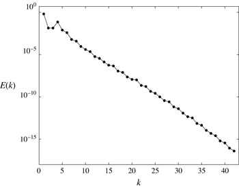
. The resulting energy spectra (cf. figure 1), and the fact that we have been able to reproduce the (relative) equilibria found by Chandler & Kerswell (Reference Chandler and Kerswell2013), reassures that
 $128^{2}$
modes are sufficient.
Typical energy spectrum of a turbulent trajectory at
 $Re=40$
.

For the time integration of the adjoint equations (3.3) and (3.9), one can take an explicit adaptive Euler time step. Denoting the right-hand side of either adjoint equation by
 $\boldsymbol{G}$
, the
 $i$
th Euler step reads
 $$\begin{eqnarray}\displaystyle \boldsymbol{u}_{i+1}=\boldsymbol{u}_{i}+{\it\delta}{\it\tau}_{i}\,\boldsymbol{G}(\boldsymbol{u}_{i}), & & \displaystyle\end{eqnarray}$$
where the length
 ${\it\delta}{\it\tau}_{i}$
of the time step is chosen small enough such that the residue
 $\Vert \boldsymbol{F}(\boldsymbol{u}_{i+1})\Vert _{\mathscr{A}}$
is less than
 $\Vert \boldsymbol{F}(\boldsymbol{u}_{i})\Vert _{\mathscr{A}}$
.
Yang & Lakoba (Reference Yang and Lakoba2007) derive an upper bound for the admissible time step
 ${\it\delta}{\it\tau}_{i}$
. Computing this upper bound for the Navier–Stokes equation is, however, not straightforward. In practice, therefore, one starts with a large value
 ${\it\delta}{\it\tau}_{i}$
and decreases it incrementally until the residue
 $\Vert \boldsymbol{F}(\boldsymbol{u}_{i+1})\Vert _{\mathscr{A}}$
reduces compared to the previous iteration.
To gain accuracy, however, we use a higher-order numerical scheme for our time integrations. This is computationally feasible due to the low cost of evaluating the right-hand sides of (3.3) and (3.9) by the pseudo-spectral method. More specifically, we use the embedded Runge–Kutta scheme RK5(4) of Dormand & Prince (Reference Dormand and Prince1980). This scheme allows for an automatic adaptive time step size. Roughly speaking, RK5(4) takes fourth- and fifth-order Runge–Kutta (RK) steps. The fifth order is eventually used for the time stepping. The fourth-order prediction is used to adjust the step size as follows. Let err denote the absolute difference between the fourth- and fifth-order predictions. Then the step size is chosen such that
 $\mathtt{err}<\mathtt{atol}+|\boldsymbol{u}_{i}|\mathtt{rtol}$
. The prescribed constants atol and rtol are the absolute and relative errors, respectively. We refer the reader to Press et al. (Reference Press, Teukolsky, Vetterling and Flannery2007, § 17.2) for further details and an implementation of the RK5(4) scheme. This integrator is also implemented in the MATLAB function ode45. For integrating the adjoint equations, we choose
 $\mathtt{atol}=\mathtt{rtol}=10^{-10}$
. Even with this conservative choice, step sizes as large as
 $10$
fictitious-time units were taken by
RK5(4).
We also use RK5(4) for the temporal discretization of the Navier–Stokes equation (4.1). However, as the time step sizes were much smaller for integrating this equation, we used the less stringent error tolerances
 $\mathtt{atol}=\mathtt{rtol}=10^{-5}$
.
4.3 Hybrid adjoint–Newton iterations
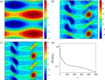
We find that the adjoint equation (3.3) does take arbitrary initial conditions to Navier–Stokes equilibria. The convergence is, however, rather slow. To demonstrate this, we take the initial condition
 $\boldsymbol{u}(\boldsymbol{x},0)=(\cos (2x_{2}),\cos (x_{1}))$
(see figure 2
a) and evolve it under the adjoint equation (3.3) to time
 ${\it\tau}=500$
. The result is shown in figure 2(b). This integration took 54 s (on an iMac with a single processor: Intel Core i5, 2.9 GHz). The
 $L^{2}$
norm of the residue
 $\boldsymbol{F}_{\mathbf{0}}$
, however, decreases to
 $\simeq 5\times 10^{-2}$
approximately, indicating that much longer integration times are required to reduce the residue sufficiently enough, say to
 $10^{-10}$
.
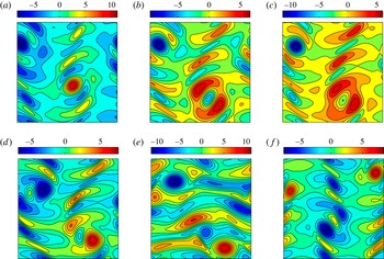
(a) The vorticity field for the initial condition
 $\boldsymbol{u}(\boldsymbol{x},0)=(\cos (2x_{2}),\cos (x_{1}))^{\text{T}}$
. (b) The initial condition evolved to time
 ${\it\tau}=500$
under the adjoint equation (3.3) to obtain
 $\boldsymbol{u}(\boldsymbol{x},500)$
. (c) The result
 $\boldsymbol{u}(\boldsymbol{x},500)$
shown in panel (b) is used as the initial guess for the Newton–GMRES–hook iterations, which converged after seven iterations with residue
 $5.98\times 10^{-11}$
. This equilibrium solution is labelled in table 1 as
 $E_{4}$
. (d) The evolution of the
 $L^{2}$
residue
 $\Vert \boldsymbol{F}_{\mathbf{0}}(\boldsymbol{u}(\cdot ,{\it\tau}))\Vert _{L^{2}}$
as the initial condition in panel (a) evolves under the adjoint equation from
 ${\it\tau}=0$
to
 ${\it\tau}=500$
.

This slow convergence is due to nearly marginal, a priori unknown eigenmodes of the adjoint operator (Lakoba & Yang Reference Lakoba and Yang2007). For particular wave equations, ad hoc methods have been proposed to eliminate these modes, and hence speed up the convergence (Yang & Lakoba Reference Yang and Lakoba2007). Owing to the complexity of the Navier–Stokes equations, it is unclear how such mode elimination techniques could be employed here.
Using the state
 $\boldsymbol{u}(\boldsymbol{x},0)=(\cos (2x_{2}),\cos (x_{1}))$
directly as the initial guess for the NGh iterations does not converge to an equilibrium either: after the first
 $20$
iterations, the residue plateaued around
 $2\times 10^{-2}$
and remained so for the
 $75$
iterations that were carried out.
Instead, when we use the result of the adjoint integration, i.e.
 $\boldsymbol{u}(\boldsymbol{x},{\it\tau}=500)$
, as the initial guess for NGh iterations, it converges after seven iterations with residue
 $5.98\times 10^{-11}$
(figure 2
c). These seven iterations took 156.84 s.
This suggests that, although the convergence of the adjoint equation to the equilibrium is slow, it takes generic initial guesses to the vicinity of the equilibrium at a relatively low computational cost. This can be seen by comparing panels (b) and (c) of figure 2, which shows that the state
 $\boldsymbol{u}(\boldsymbol{x},{\it\tau}=500)$
is quite similar to the equilibrium
 $E_{4}$
, and thus likely to lie in its NGh domain of attraction. Indeed, switching to NGh took this state to the equilibrium solution within a few iterations.
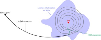
State space depiction of the hybrid adjoint–Newton method. An initial guess may be too far away from the desired equilibrium solution EQ for the Newton–GMRES–hook iterations (NGh) to converge to it. The adjoint descent may eventually converge to EQ, but alone it would take a long integration time to do so. In the hybrid adjoint–Newton method the adjoint descent takes the initial guess to the domain of attraction of NGh. Once there, NGh converges to EQ in a few iterations.

Based on this observation, we propose the following hybrid adjoint–Newton iterations, sketched in figure 3. We take a prescribed positive real number
 ${\it\tau}_{0}$
and a positive integer N. An initial condition
 $\boldsymbol{u}(\boldsymbol{x},0)$
is then integrated under the adjoint equation (3.3) to obtain
 $\boldsymbol{u}(\boldsymbol{x},{\it\tau}_{0})$
. This state is then fed into the NGh algorithm and N iterations of NGh are performed. The output is then fed back into the adjoint equation as the initial condition. This hybrid loop is repeated until the residue
 $\Vert \boldsymbol{F}_{\mathbf{0}}\Vert _{L^{2}}$
decreases below some prescribed tolerance tol. This procedure is summarized in Algorithm 1. The hybrid adjoint–Newton iterations for finding travelling waves are similar except that the adjoint equations (3.9) are solved at each iteration (see Algorithm 2).


For the computations reported below, we set
 ${\it\tau}_{0}=100$
,
 $\mathtt{tol}=10^{-10}$
and
 $\mathtt{N}=1$
. Since NGh steps are relatively expensive, we only take one NGh step (
 $\mathtt{N}=1$
) per iteration of adjoint–Newton. At Reynolds number
 $Re=40$
, for instance, the integration of the adjoint equations to
 ${\it\tau}=100$
took approximately 10 s on average while each NGh step took approximately 50 s on average.
4.4 Equilibrium solutions
In this section, we report the equilibria found by the hybrid adjoint–Newton iterations (Algorithm 1). We also compare its performance with that of pure NGh iterations without the adjoint step.
To this end, we consider the set of initial guesses
 $$\begin{eqnarray}\displaystyle \boldsymbol{u}_{0}^{(m_{1},m_{2})}=(\cos (m_{2}x_{2}),\cos (m_{1}x_{1})), & & \displaystyle\end{eqnarray}$$
for a range of integers
 $m_{1}$
and
 $m_{2}$
. We find that for
 $m_{2}>4$
, both Newton–GMRES–hook and the hybrid adjoint–Newton iterations converge to the laminar equilibrium
 $E_{0}$
. Therefore, we restrict the range of the integers to
 $1\leqslant m_{1},m_{2}\leqslant 4$
. This leads to
 $16$
distinct initial guesses.
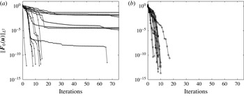
The decay of the residue (i.e. the
 $L^{2}$
-norm of the right-hand side) using Newton–GMRES–hook iterations (a) and the hybrid adjoint–Newton iterations (b).

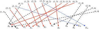
The convergence diagram. Double indices
 $(m_{1},m_{2})$
label the initial guesses (4.7). A dashed black arrow indicates that both the hybrid adjoint–Newton and the NGh iterations converge to the same equilibrium. A dotted blue arrow indicates that the NGh iterations converge to a different equilibrium from the one reached by the hybrid adjoint–Newton (red arrow). A solid red arrow (with no blue arrow originating from the same initial guess) indicates that only the hybrid adjoint–Newton converged to the equilibrium, i.e. the NGh iterations alone failed to converge.

These initial conditions are divergence-free by construction, consistent with our incompressible Navier–Stokes setting. They are also explicit, rendering the following results reproducible. Furthermore, the generic nature of the initial conditions illustrates the main advantage of the adjoint descent method, namely that its convergence does not require good initial guesses. For brevity, we shall refer to the states
 $\boldsymbol{u}_{0}^{(m_{1},m_{2})}$
by their indices
 $(m_{1},m_{2})$
.
Using the hybrid adjoint–Newton iterations for equilibria (see Algorithm 1), all
 $16$
runs converged, resulting in
 $10$
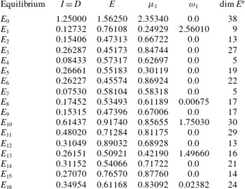
distinct equilibria. These equilibria are listed as
 $E_{0}$
to
 $E_{9}$
in table 1, where
 $E_{0}$
is the laminar state (4.2). All initial guesses converged to an equilibrium within the first
 $10$
iterations of hybrid adjoint–Newton iterations, except initial guess
 $(2,1)$
which took
 $17$
iterations (see figure 4). Figure 5 shows the convergence diagram, connecting each initial guess
 $(m_{1},m_{2})$
to the resulting equilibrium solution.
Using NGh alone, only nine out of
 $16$
runs converged. They converged to seven distinct equilibria:
 $E_{0}$
,
 $E_{1}$
,
 $E_{6}$
,
 $E_{8}$
,
 $E_{9}$
,
 $E_{10}$
and
 $E_{11}$
(see figure 5). This comes initially as a surprise since the exhaustive search carried out by Chandler & Kerswell (Reference Chandler and Kerswell2013) only returned a single equilibrium (i.e.
 $E_{1}$
). This can be explained, however, in terms of the method used for initiating the NGh iterations. Chandler & Kerswell (Reference Chandler and Kerswell2013) use recurrences to find initial guesses for their searches, as opposed to the generic initial guesses used here. Recurrences only happen in a subset of the state space where a generic turbulent trajectory spends most of its lifetime. As a result, using recurrences for initiating the NGh searches might preferentially yield the equilibria ‘close’ to this region. We will return to this subject in § 5, where the temporal intermittency is discussed.
We also sought further equilibria using states of the form
 $(\sin (m_{2}x_{2}),\cos (m_{1}x_{1}))$
as the initial guesses for the hybrid adjoint–Newton iterations. This resulted in five more equilibria:
 $E_{12}$
to
 $E_{16}$
in table 1. While all of these additional searches did converge, most of them re-converged to previously discovered equilibria, including
 $E_{10}$
and
 $E_{11}$
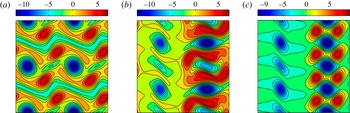
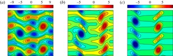
that were only found by NGh iterations when initial guesses (4.7) were used. Figure 6 shows the vorticity field of three select equilibrium solutions.
Vorticity fields of the equilibrium solutions
 $E_{5}$
(a),
 $E_{12}$
(b) and
 $E_{15}$
(c). All panels show the entire domain
 $[0,2{\rm\pi}]\times [0,2{\rm\pi}]$
.

List of equilibrium solutions at
 $Re=40$
. Energy
 $E$
, energy dissipation
 $D$
and energy input
 $I$
are defined in (4.3). The leading unstable eigenvalue of the equilibrium is
 ${\it\mu}_{1}+\text{i}{\it\omega}_{1}$
. The dimension of the linear unstable manifold of the equilibrium is denoted by
 $\dim E^{u}$
.

Vorticity fields of the equilibrium solutions at Reynolds number
 $Re=60$
(a),
 $Re=80$
(b) and
 $Re=100$
(c). All panels show the entire
 $[0,2{\rm\pi}]\times [0,2{\rm\pi}]$
domain.

Some of the equilibria (e.g.
 $E_{15}$
shown in figure 6) exhibit vertical bands of localized vorticity that are separated by an almost zero-vorticity background. Such spatially localized equilibria of the Kolmogorov flow were only observed previously on domains with small aspect ratio
 ${\it\alpha}=L_{2}/L_{1}$
(Lucas & Kerswell Reference Lucas and Kerswell2014). The fact that they also exist on a domain with aspect ratio
 ${\it\alpha}=1$
comes as a surprise.
Although our focus here is on Reynolds number
 $Re=40$
, figure 7 showcases select equilibria at
 $Re=60$
,
 $80$
and
 $100$
. These equilibria are computed using the higher resolution of
 $256\times 256$
Fourier modes. They are found by our hybrid adjoint–Newton method while the previous studies using Newton–GMRES–hook iterations had not been able to discover them (Chandler & Kerswell Reference Chandler and Kerswell2013).
4.5 Travelling-wave solutions
The forcing term in the Kolmogorov equation (4.1) breaks the continuous symmetry in the
 $x_{2}$
direction. Therefore, only travelling-wave solutions of the type
 $\boldsymbol{u}(\boldsymbol{x}-\boldsymbol{c}t)$
with
 $\boldsymbol{c}=(c,0)$
are permitted. This reduces the wave velocity equations (3.9b
) to the scalar equation
 $$\begin{eqnarray}\displaystyle \frac{\text{d}c}{\text{d}{\it\tau}}=-\int _{\mathbb{T}^{2}}\frac{\partial \boldsymbol{u}}{\partial x_{1}}\boldsymbol{\cdot }\tilde{\boldsymbol{u}}^{\prime \prime }\,\text{d}^{2}\boldsymbol{x}. & & \displaystyle\end{eqnarray}$$
Similarly, the term
 $\boldsymbol{c}\boldsymbol{\cdot }\boldsymbol{{\rm\nabla}}\tilde{\boldsymbol{u}}^{\prime \prime }$
in (3.9a
) reduces to
 $c\,\partial _{x_{1}}\tilde{\boldsymbol{u}}^{\prime \prime }$
and the term
 $\boldsymbol{c}\boldsymbol{\cdot }\boldsymbol{{\rm\nabla}}\boldsymbol{u}$
in (3.10) reduces to
 $c\,\partial _{x_{1}}\boldsymbol{u}$
.
We search for travelling waves using Algorithm 2 and the generic initial guesses discussed in the previous section. For the initial wave speed, we used
 $c(0)=1$
. Other values of
 $c(0)$
yielded similar results.
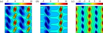
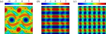
Vorticity field for the travelling-wave solutions
 $T_{4}$
(a),
 $T_{7}$
(b) and
 $T_{8}$
(c). All panels show the entire domain
 $[0,2{\rm\pi}]\times [0,2{\rm\pi}]$
.

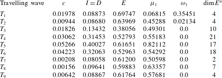
List of travelling-wave solutions at
 $Re=40$
. The constant
 $c$
denotes the wave speed. Energy
 $E$
, energy dissipation
 $D$
and energy input
 $I$
are defined in (4.3). The leading unstable eigenvalue of the travelling wave is
 ${\it\mu}_{1}+\text{i}{\it\omega}_{1}$
. The dimension of the linear unstable manifold of the travelling wave is denoted by
 $\dim E^{u}$
.

Some of our searches for travelling waves converged to equilibrium solutions. This is to be expected, as equilibria are degenerate travelling waves with wave speed
 $c=0$
. In fact, the adjoint equation (3.9) admits such solutions. This can be readily verified by letting
 $\boldsymbol{u}(\boldsymbol{x})$
be an equilibrium solution of the Navier–Stokes equation and setting
 $\boldsymbol{c}\equiv 0$
. Then
 $\boldsymbol{u}^{\prime \prime }$
in (3.10) is zero, resulting in vanishing right-hand sides in (3.9).
Nonetheless, our hybrid adjoint–Newton searches led to nine distinct travelling waves listed in table 2. Only travelling waves
 $T_{1}$
and
 $T_{2}$
had been discovered previously (Chandler & Kerswell Reference Chandler and Kerswell2013). Figure 8 shows the vorticity field for three select travelling waves. As in the case of equilibria, we find that some of the travelling waves (e.g.
 $T_{8}$
in figure 8) exhibit localized spatial structures, although the domain aspect ratio is one.
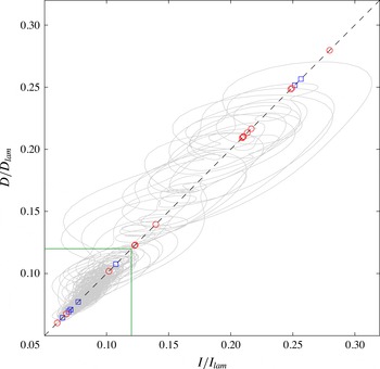
Results for
 $Re=40$
. Grey curve: turbulent trajectory spanning
 $10^{3}$
time units. Red circles: equilibria. Blue squares: travelling waves. The green square marks the region where
 $I/I_{lam}<0.12$
and
 $D/D_{lam}<0.12$
. The turbulent trajectory spends
 $86.62\,\%$
of the total
 $10^{3}$
time units inside this region. The diagonal
 $I=D$
is marked by the dashed black line. Equilibria and travelling waves with
 $I/I_{lam}=D/D_{lam}>0.32$
are not shown.

5 Temporal intermittency in Kolmogorov flow
In this section, we explore the significance of the invariant solutions, found in the previous section, on the global dynamics of the Kolmogorov flow.
Figure 9 shows the energy input
 $I$
versus the energy dissipation
 $D$
for a generic turbulent trajectory computed for
 $10^{3}$
time units and recorded every
 $0.1$
time units. The energy input and dissipation of each equilibrium and travelling wave are marked by circles and squares, respectively. As mentioned earlier, the energy input and dissipation coincide for these invariant solutions, locating them on the diagonal
 $I=D$
.
The equilibria and travelling waves assume a wide range of energy input and dissipation. The turbulent trajectory, on the other hand, mostly resides in a relatively low energy input–dissipation regime. In particular, approximately
 $85\,\%$
of this trajectory belongs to the
 $I/I_{lam}<0.12$
and
 $D/D_{lam}<0.12$
regime, marked by the green square in figure 9. For the lack of a better term, we refer to this regime as the ‘ergodic sea’.
At the same time, the turbulent trajectory also experiences sporadic episodes of high energy input and dissipation. Such rare, extreme events are usually referred to as temporal intermittency and are ubiquitous in turbulent fluid flow (see e.g. Batchelor & Townsend Reference Batchelor and Townsend1949; Sreenivasan & Antonia Reference Sreenivasan and Antonia1997). Non-Gaussian probability distributions of turbulent quantities are a footprint of intermittency that produces the heavy tails of the distribution functions (Frisch Reference Frisch1996; Mininni & Pouquet Reference Mininni and Pouquet2010).
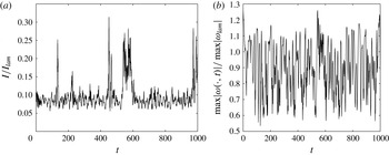
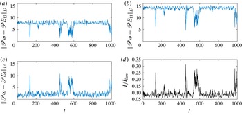
The short lifetime of the intermittent bursts is better seen in figure 10(a) where the normalized energy input
 $I/I_{lam}$
is shown as a function of time. The time series for the energy dissipation (not shown here) is very similar, except that the intermittent bursts of the dissipation occur with a short delay of
 $0.5$
to
 $1.5$
time units relative to the energy input bursts. This suggests that, once in a while, the turbulent velocity field mostly aligns with the external forcing
 $\sin (nx_{2})\boldsymbol{e}_{1}$
, resulting in the growth of the energy input, which kicks the trajectory out of its ergodic sea. After a short time delay, the energy dissipation also increases, bringing the trajectory back to the ergodic regime.
Spatial intermittency is also a characteristic of turbulent fluid flow, which refers to unusually large velocity (or vorticity) amplitudes occurring in a relatively small subset of the physical domain (see e.g. Kuo & Corrsin Reference Kuo and Corrsin1971; Schneider, Farge & Kevlahan Reference Schneider, Farge and Kevlahan2004; Ruppert-Felsot, Farge & Petitjeans Reference Ruppert-Felsot, Farge and Petitjeans2009). Although temporal and spatial intermittencies are sometimes conflated in the literature, the relation between the two is not well understood (Gibbon & Doering Reference Gibbon and Doering2003). For our turbulent trajectory, in fact, an appreciable correlation between them was not found. Figure 10(b), for instance, shows that the normalized maximum vorticity amplitude oscillates rapidly throughout the simulation time, exhibiting no clear correlation with the energy input.
Focusing on the temporal intermittency, we first review the dynamical systems perspective of this phenomena.
(a) The energy input
 $I$
as a function of time normalized by the energy input of the laminar state
 $I_{lam}=1.25$
. (b) The spatial maximum of vorticity magnitude, i.e.
 $\max _{\boldsymbol{x}\in \mathbb{T}^{2}}|{\it\omega}(\boldsymbol{x},t)|$
, normalized by its value corresponding to the laminar state, i.e.
 $\max _{\boldsymbol{x}\in \mathbb{T}^{2}}|{\it\omega}_{lam}(\boldsymbol{x})|=10$
.

5.1 A dynamical systems perspective on temporal intermittency
Although the Navier–Stokes equations generate an infinite-dimensional dynamical system, it is believed that, owing to the dissipative term
 ${\it\nu}{\rm\Delta}\boldsymbol{u}$
, its solutions converge exponentially fast to a finite-dimensional, invariant set, usually referred to as the inertial manifold (see Constantin et al. (Reference Constantin, Foias, Nicolaenko and Temam1989) for the rigorous definition). The existence of the inertial manifold for the Navier–Stokes equation, in its most general form, is an open mathematical problem. In practice, however, its existence is often assumed. In fact, this assumption underlies the finite Galerkin truncations used in computations (Foias et al.
Reference Foias, Jolly, Kevrekidis, Sell and Titi1988).
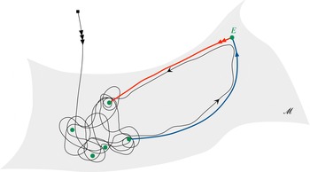
Some (relative) equilibria and (relative) periodic orbits and portions of their stable and unstable manifolds belong to the inertial manifold. For large enough Reynolds numbers, these invariant solutions are typically unstable. A generic turbulent trajectory visits the neighbourhood of an invariant solution for a finite time before it is repelled along its unstable manifold towards the neighbourhood of another invariant solution (Ruelle Reference Ruelle and Sirovich1991; Halcrow et al. Reference Halcrow, Gibson, Cvitanović and Viswanath2009). This process continues indefinitely in a somewhat unpredictable fashion, thereby causing the complex temporal behaviour of turbulent trajectories (see figure 11 for an illustration).
An initial condition (black square) decays rapidly to the inertial manifold
 $\mathscr{M}$
where the dynamics is governed by the (relative) equilibria, (relative) periodic orbits and portions of their stable/unstable manifolds that lie within the inertial manifold. The green dots represent equilibria. Highly unstable invariant solutions (e.g. the equilibrium
 $E$
) are rarely visited by a generic trajectory.

From this perspective, intermittent episodes are viewed as close passages of the turbulent trajectory to invariant solutions that reside in a ‘less accessible’ region of the inertial manifold or, more precisely, the attractor (Holmes Reference Holmes1993). As depicted in figure 11, such passages are viable along the heteroclinic connections between the invariant solutions (Holmes & Stone Reference Holmes, Stone, Gatski, Speziale and Sarkar1992; Holmes et al. Reference Holmes, Lumley, Berkooz and Rowley2012).
To characterize the less accessible regions of the attractor, one naturally needs to answer the following question: how frequently is an invariant solution visited by generic turbulent trajectories? There is no straightforward, a priori answer to this question (Cvitanović et al.
Reference Cvitanović, Artuso, Mainieri, Tanner and Vattay2014, ch. 23). There are, however, some characteristics of the invariant solutions that are relevant. In tables 1 and 2, for instance, we report the dimension of the linear unstable manifold (i.e.
 $\dim E^{u}$
) of each invariant solution. The invariant solutions
 $E_{1}$
,
 $E_{4}$
,
 $E_{7}$
,
 $T_{1}$
,
 $T_{2}$
,
 $T_{3}$
,
 $T_{7}$
,
 $T_{8}$
and
 $T_{9}$
that reside close to the ergodic sea have at most
 $10$
linearly unstable eigenmodes. The remaining invariant solutions have at least
 $13$
unstable eigenmodes and seem to reside further away from the ergodic sea.
In tables 1 and 2, we also report the stability exponent
 ${\it\mu}_{1}+\text{i}{\it\omega}_{1}$
of the most unstable eigenmode of each invariant solution. It is tempting to assert that the invariant solutions with larger
 ${\it\mu}_{1}$
are less likely to be visited by a generic turbulent trajectory. This is, however, not the case. For instance, we have
 ${\it\mu}_{1}=0.62697$
for equilibrium
 $E_{4}$
and
 ${\it\mu}_{1}=0.61189$
for equilibrium
 $E_{8}$
. Equilibrium
 $E_{4}$
is located in the heart of the ergodic sea and is, in fact, visited by the turbulent trajectory quite often. Equilibrium
 $E_{8}$
, in spite of having a similar stability exponent, is rarely visited by the turbulent trajectory. The crucial difference between these two equilibria is the dimension of the linear unstable manifold, which is
 $\dim E^{u}=5$
for
 $E_{4}$
and
 $\dim E^{u}=17$
for
 $E_{8}$
.
In retrospect, the lack of correlation between the stability exponent and the frequency of visitations by the turbulent trajectory is to be expected. The stability exponent of an invariant solution is a local quantity. As such, for it to be meaningful, the turbulent trajectory should already be in the vicinity of the invariant solution. Once there, the stability exponent
 ${\it\mu}_{1}$
determines how quickly the trajectory will leave the neighbourhood.
At any rate, neither the dimension of the unstable manifold nor the stability exponents of an invariant solution decisively determine the frequency at which its neighbourhood is visited by a turbulent trajectory. Therefore, we take a more direct approach to quantify intermittency. Namely, we measure the
 $L^{2}$
distance between the turbulent trajectory and the computed invariant solutions.
The Kolmogorov equation is equivariant under a one-parameter family of continuous symmetries and a number of discrete symmetries (Sirovich Reference Sirovich1987). This implies that each solution
 $\boldsymbol{u}(t)$
has infinitely many equivalent copies. Therefore, when measuring the ‘distance’ between two states, one needs to make an informed choice among the equivalent copies of each state. This necessitates a discussion on the symmetries of the Kolmogorov flow.
5.2 Symmetries of Kolmogorov flow
The Kolmogorov equation (4.1) is equivariant with respect to
 $4n$
discrete symmetries and a continuous translational symmetry (Sirovich Reference Sirovich1987). We denote the complete set of such symmetries by
 $$\begin{eqnarray}\displaystyle & \displaystyle (\mathscr{T}_{\ell }\boldsymbol{u})(x_{1},x_{2})=\boldsymbol{u}(x_{1}+\ell ,x_{2}), & \displaystyle\end{eqnarray}$$
 $$\begin{eqnarray}\displaystyle & \displaystyle (\mathscr{R}\boldsymbol{u})(x_{1},x_{2})=-\boldsymbol{u}(-x_{1},-x_{2}), & \displaystyle\end{eqnarray}$$
 $$\begin{eqnarray}\displaystyle & \displaystyle (\mathscr{S}^{m}\boldsymbol{u})(x_{1},x_{2})=\left(\begin{array}{@{}c@{}}(-1)^{m}u_{1}((-1)^{m}x_{1},x_{2}+m{\rm\pi}/n)\\ u_{2}((-1)^{m}x_{1},x_{2}+m{\rm\pi}/n)\end{array}\right), & \displaystyle\end{eqnarray}$$
 $m\in \{0,1,\ldots ,2n-1\}$
. Here,
 $\mathscr{T}_{\ell }$
denotes
 $\ell$
shift in the
 $x_{1}$
direction,
 $\mathscr{R}$
denotes rotation through
 ${\rm\pi}$
and
 $\mathscr{S}$
denotes a simultaneous
 $({\rm\pi}/n)$
shift in the
 $x_{2}$
direction and a reflection in the
 $x_{1}$
direction.
One can readily verify that the above symmetry operations act on the vorticity field according to the following rules:
 $$\begin{eqnarray}\displaystyle & \displaystyle (\mathscr{T}_{\ell }{\it\omega})(x_{1},x_{2})={\it\omega}(x_{1}+\ell ,x_{2}), & \displaystyle\end{eqnarray}$$
 $$\begin{eqnarray}\displaystyle & \displaystyle (\mathscr{R}{\it\omega})(x_{1},x_{2})={\it\omega}(-x_{1},-x_{2}), & \displaystyle\end{eqnarray}$$
 $$\begin{eqnarray}\displaystyle & \displaystyle (\mathscr{S}^{m}{\it\omega})(x_{1},x_{2})=(-1)^{m}{\it\omega}((-1)^{m}x_{1},x_{2}+m{\rm\pi}/n). & \displaystyle\end{eqnarray}$$
The glide reflection (or shift–reflect operation)
 $\mathscr{S}$
generates a cyclic group of order
 $2n$
,
 $$\begin{eqnarray}\displaystyle C_{2n}=\{e,\mathscr{S},\mathscr{S}^{2},\ldots ,\mathscr{S}^{2n-1}\}, & & \displaystyle\end{eqnarray}$$
where
 $e$
denotes the identity
 $e=\mathscr{S}^{0}$
. The rotation-through-
 ${\rm\pi}$
operation
 $\mathscr{R}$
generates a cyclic group of order two,
 $R_{2}=\{e,\mathscr{R}\}$
. The complete set of discrete symmetries of the Kolmogorov equation, therefore, is the dihedral group of order
 $4n$
, i.e.
 $$\begin{eqnarray}\displaystyle D_{4n}=R_{2}\ltimes C_{2n}=\{e,\mathscr{S},\ldots ,\mathscr{S}^{2n-1},\mathscr{R},\mathscr{R}\mathscr{S},\ldots ,\mathscr{R}\mathscr{S}^{2n-1}\}. & & \displaystyle\end{eqnarray}$$
Note that the operations
 $\mathscr{R}$
and
 $\mathscr{S}$
do not commute,
 $\mathscr{R}\mathscr{S}\neq \mathscr{S}\mathscr{R}$
. Instead, we have
 $\mathscr{S}\mathscr{R}\mathscr{S}=\mathscr{R}$
.
Therefore, the solutions of the Kolmogorov equation have up to
 $4n$
distinct but equivalent copies due to its equivariance under the discrete symmetries
 $D_{4n}$
. They also have infinitely many equivalent copies due to the continuous symmetry
 $\mathscr{T}_{\ell }$
for any
 $\ell \in [0,2{\rm\pi}]$
.
An invariant solution may itself have some, all or none of the symmetries of the equations. The laminar solution
 $E_{0}$
, for instance, has the complete set of symmetries, i.e.
 $gE_{0}=E_{0}$
for all
 $g\in D_{4n}$
and
 $\mathscr{T}_{\ell }E_{0}=E_{0}$
for all
 $\ell \in [0,2{\rm\pi}]$
. The laminar state, therefore, has only one copy. The travelling wave
 $T_{7}$
(see figure 8), on the other hand, has no symmetries and therefore possesses infinitely many equivalent copies. Incidentally, travelling wave
 $T_{7}$
happens to have the lowest-dimensional unstable manifold,
 $\dim E^{u}=2$
, among the solutions found here.
These symmetry-related copies greatly complicate the analysis of the state space of the Kolmogorov flow. When comparing the
 $L^{2}$
distance between two states
 $\boldsymbol{u}^{1}$
and
 $\boldsymbol{u}^{2}$
, one needs to take the minimum
 $L^{2}$
distance between
 $\boldsymbol{u}^{1}$
and
 $\boldsymbol{u}^{2}$
and all their symmetry-related copies. For example, let
 $\boldsymbol{u}^{2}(t)$
be a symmetry copy of a solution
 $\boldsymbol{u}^{1}(t)$
such that
 $\boldsymbol{u}^{2}(t)=(\mathscr{T}_{\ell }\boldsymbol{u}^{1})(t)$
for some
 $\ell \in (0,2{\rm\pi})$
. These two states are equivalent and both solve the Kolmogorov equation. However, the norm
 $\Vert \mathscr{T}_{\ell }\boldsymbol{u}^{1}-\boldsymbol{u}^{1}\Vert _{L^{2}}$
is generally non-zero. Therefore, an appropriate norm on the state space of the Kolmogorov flow is
 $$\begin{eqnarray}\displaystyle \min \Vert \boldsymbol{u}^{1}-g\mathscr{T}_{\ell }\boldsymbol{u}^{2}\Vert _{L^{2}}, & & \displaystyle\end{eqnarray}$$
where the minimum is taken over all
 $\ell \in [0,2{\rm\pi}]$
and
 $g\in D_{4n}$
. Evaluating this norm can be somewhat cumbersome.
Another approach is to map each state into a symmetry-invariant polynomial basis. For low-dimensional dynamical systems with simple discrete symmetries, such coordinates are available analytically (Gilmore & Letellier Reference Gilmore and Letellier2007). As the dimension of the system (and/or the order of the group) increases, the determination of the invariant coordinates becomes quickly prohibitive (Siminos & Cvitanović Reference Siminos and Cvitanović2011). As a result, and to the best of our knowledge, symmetry-invariant polynomial coordinates for the Kolmogorov flow are not known.
Here, we take an alternative approach, which also proves to be insightful in analysis of the temporal intermittency. We define the projection operator
 $$\begin{eqnarray}\displaystyle \mathscr{P}\boldsymbol{u}=\frac{1}{4n}\mathop{\sum }_{m=0}^{2n-1}\mathscr{S}^{m}(\boldsymbol{u}+\mathscr{R}\boldsymbol{u}), & & \displaystyle\end{eqnarray}$$
which is the average over all copies of
 $\boldsymbol{u}$
given by the discrete symmetries
 $D_{4n}$
(Cvitanović et al.
Reference Cvitanović, Artuso, Mainieri, Tanner and Vattay2014). The projection
 $\mathscr{P}\boldsymbol{u}$
is invariant under all discrete symmetries
 $g\in D_{4n}$
and therefore we refer to it as the symmetric part of the state
 $\boldsymbol{u}$
. The symmetric part of vorticity
 ${\it\omega}$
is defined analogously.
All
 $4n$
symmetry copies of the state
 $\boldsymbol{u}$
have a unique projection
 $\mathscr{P}\boldsymbol{u}$
. Working with the symmetric part of the states, therefore, eliminates the complications arising from the discrete symmetries.
Considering this symmetric part also has a physical motivation. The energy
 $E$
, dissipation
 $D$
and energy input
 $I$
defined in (4.3) are invariant under symmetry operations. Denoting the energy input of a state
 $\boldsymbol{u}$
by
 $I[\boldsymbol{u}]$
, we have
 $I[\boldsymbol{u}]=I[g\boldsymbol{u}]$
for
 $g$
being any symmetry of the Kolmogorov flow. The same holds for energy
 $E$
and dissipation
 $D$
. The particular linear form of the energy input
 $I[\boldsymbol{u}]$
implies that it is also invariant under the projection operation
 $\mathscr{P}$
, i.e.
 $I[\boldsymbol{u}]=I[\mathscr{P}\boldsymbol{u}]$
.
Furthermore, we have
 $$\begin{eqnarray}\displaystyle I[\boldsymbol{u}-\mathscr{P}\boldsymbol{u}]=0, & & \displaystyle\end{eqnarray}$$
that is, the remainder
 $\boldsymbol{u}-\mathscr{P}\boldsymbol{u}$
does not contribute to the energy input. As discussed in § 5.1, the intermittent episodes of the flow are triggered by high energy inputs. Therefore, to study the temporal intermittency of the Kolmogorov flow, it is sufficient to consider the symmetric part
 $\mathscr{P}\boldsymbol{u}$
. Note, however, that, owing to the quadratic form of
 $E$
and
 $D$
, the energy and dissipation of the remainder
 $\boldsymbol{u}-\mathscr{P}\boldsymbol{u}$
are generally non-zero.
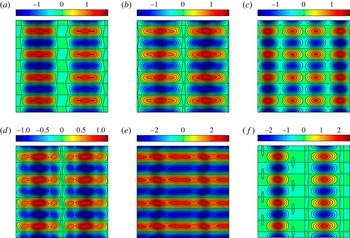
The symmetric part of the vorticity field
 $\mathscr{P}{\it\omega}$
of the turbulent trajectory at
 $t=84$
(a),
 $t=94$
(b),
 $t=104$
(c),
 $t=124.2$
(d),
 $t=134.2$
(e) and
 $t=144.2$
(f). The energy input–dissipation pairs
 $(I,D)$
for the states are
 $(0.109,0.107)$
,
 $(0.115,0.114)$
,
 $(0.104,0.104)$
,
 $(0.095,0.094)$
,
 $(0.314,0.269)$
and
 $(0.099,0.093)$
, respectively.

The remaining continuous symmetry
 $\mathscr{T}_{\ell }$
is handled here by the method of slices (Cartan Reference Cartan1935; Field Reference Field1980; Rowley et al.
Reference Rowley, Kevrekidis, Marsden and Lust2003). This method replaces all continuous symmetry copies of a state with a copy that belongs to a given hypersurface called the slice. This hypersurface is such that each group orbit
 $\mathscr{T}_{\ell }\boldsymbol{u}$
in a neighbourhood of a given state intersects the slice transversely at a unique point. Each group orbit
 $\mathscr{T}_{\ell }\boldsymbol{u}$
is then replaced by its unique intersection with the slice. The method of slices has only recently been used in the context of fluid dynamics (Willis et al.
Reference Willis, Cvitanović and Avila2013; Willis, Short & Cvitanović Reference Willis, Short and Cvitanović2015). We use the first-Fourier-mode implementation of this method developed by Budanur et al. (Reference Budanur, Cvitanović, Davidchack and Siminos2015) (cf. appendix D for more detail).
5.3 Temporal intermittency
Figure 12 shows the symmetric part of the vorticity field
 $\mathscr{P}{\it\omega}$
for six select times along the turbulent trajectory. Since the forcing wavenumber is
 $n=4$
, there are
 $4n=16$
discrete symmetries. As a result, the symmetric part of each state exhibits recurring patterns that are related through discrete symmetry operations
 $\mathscr{R}$
and
 $\mathscr{S}$
. In other words, knowing the symmetric part
 $\mathscr{P}{\it\omega}$
on one-sixteenth of the domain
 $[0,2{\rm\pi}]\times [0,2{\rm\pi}]$
, one can reproduce
 $\mathscr{P}{\it\omega}$
on the entire domain.
The vorticity field
 ${\it\omega}$
for the snapshots of the turbulent trajectory shown in figure 12. The panels correspond to times
 $t=84$
(a),
 $t=94$
(b),
 $t=104$
(c),
 $t=124.2$
(d),
 $t=134.2$
(e) and
 $t=144.2$
(f).

Figure 12(e), showing the state at time
 $t=134.2$
, corresponds to the first intermittent peak in figure 10(a). A distinct change of topology occurs in the symmetric part of the vorticity field as the turbulent trajectory undergoes an intermittent episode. Before and after the episode,
 $\mathscr{P}{\it\omega}$
has at least two distinct co-rotating vortices in each positive (or negative) vorticity band. As the trajectory gets closer to the intermittent episode, the co-rotating vortices merge, resulting in horizontal bands of alternating positive and negative vorticity. After the episode (see figure 12
f), these bands split again into two distinct co-rotating vortices. This sharp distinction is not immediate from the full vorticity field
 ${\it\omega}$
(cf. figure 13). The same trend (i.e. the merger of co-rotating vortices) was observed during the intermittent episodes occurring at later times.
(a) The vorticity field
 ${\it\omega}$
for the equilibrium solution
 $E_{13}$
. (b) The symmetric part of the vorticity
 $\mathscr{P}{\it\omega}$
for the equilibrium solution
 $E_{13}$
. (c) The symmetric part of the vorticity
 $\mathscr{P}{\it\omega}$
for the equilibrium solution
 $E_{6}$
.

We found by inspection that the symmetric part of equilibrium solution
 $E_{13}$
(see figure 14) is strikingly similar to that of the turbulent trajectory as it undergoes intermittency. This is visually appreciable from comparing figure 12(e) with figure 14(b). This observation suggests that close passages to equilibrium
 $E_{13}$
trigger the intermittent behaviour.
In figure 14(c), we also show the symmetric part
 $\mathscr{P}{\it\omega}$
for equilibrium
 $E_{6}$
. While the energy input–dissipation of equilibria
 $E_{6}$
and
 $E_{13}$
are very close (cf. table 1), their vorticity fields are very different. This demonstrates the fact that closeness of the energy input–dissipation of two states does not imply their closeness in the state space.
To quantitatively examine the role of equilibrium
 $E_{13}$
on intermittency, we consider the
 $L^{2}$
distance between the symmetric part of each turbulent state and the symmetric part of equilibrium
 $E_{13}$
, i.e.
 $\Vert \mathscr{P}{\it\omega}(t)-\mathscr{P}E_{13}\Vert _{L^{2}}$
. To account for the continuous translational symmetry, each symmetric part is first brought to the first-Fourier-mode slice, as explained in appendix D, before the distance is computed.
The
 $L^{2}$
distance
 $\Vert \mathscr{P}{\it\omega}(t)-\mathscr{P}E\Vert _{L^{2}}$
between the symmetric part of the turbulent trajectory
 $\mathscr{P}{\it\omega}$
and the symmetric parts of the equilibria
 $E_{13}$
(a),
 $E_{11}$
(b) and
 $E_{1}$
(c). (d) The normalized energy input
 $I/I_{lam}$
of the turbulent trajectory, shown for reference (same as figure 10
a). Each distinguished peak of the energy input (i.e. intermittency) coincides with a significant decrease in the distance from the equilibrium
 $E_{13}$
.

Figure 15 shows the evolution of the
 $L^{2}$
distance as a function of time. The evolution of the energy input
 $I$
is also shown in the same figure. Every intermittent episode, i.e. significant peaks in the energy input, is concurrent with a significant dip in the
 $L^{2}$
distance. This demonstrates that the intermittent episodes correspond to close passages of the turbulent trajectory to equilibrium
 $E_{13}$
.
The distance between the turbulent trajectory and some of the other invariant solutions (e.g.
 $E_{11}$
and
 $T_{4}$
) also decreases during the intermittent episodes. Their decrease is, however, not as dramatic as the one observed for equilibrium
 $E_{13}$
. For instance, the evolution of the distance from
 $E_{11}$
is also shown in figure 15. The distance from
 $E_{11}$
fluctuates mostly around
 $14.0$
, which is significantly larger than the average distance from
 $E_{13}$
, which fluctuates around
 $8.0$
. During the intermittent episodes, the distance from both equilibria decreases. The distance from
 $E_{11}$
reaches
 $4.64$
at its minimum, which is approximately one-third of its average distance of
 $14.0$
. The decrease in the distance from
 $E_{13}$
is more significant: it attains a minimum as low as
 $1.21$
, which is approximately
 $6.6$
times smaller than its average distance of
 $8.0$
. In contrast, the distance from equilibria residing in the ergodic sea increases during each intermittent episode. The distance from the equilibrium
 $E_{1}$
is shown in figure 15 as an example.
If the Kolmogorov flow at Reynolds number
 $Re=40$
possesses an ergodic attractor, as the numerical evidence suggests (see e.g. Platt et al.
Reference Platt, Sirovich and Fitzmaurice1991), every invariant solution embedded in the attractor will eventually be visited by a generic turbulent trajectory. Nonetheless, for the finite-time (and relatively short) turbulent trajectory computed here, equilibrium
 $E_{13}$
appears to explain its observed intermittencies.
Finding the invariant equilibrium and travelling-wave solutions is only the first step. A complete understanding of the Kolmogorov flow in terms of its invariant solutions will require a detailed state space analysis of the type carried out by Gibson, Halcrow & Cvitanović (Reference Gibson, Halcrow and Cvitanović2008) for the plane Couette flow. Such a thorough study deserves its own treatment, which will be presented elsewhere.
6 Conclusions and perspectives
We have proposed and developed here a new method for finding the equilibrium and travelling-wave (relative equilibrium) solutions of the forced Navier–Stokes equations with periodic boundary conditions. Namely, adjoint PDEs were derived whose (relative) equilibria include those of Navier–Stokes equations. Furthermore, the (relative) equilibria of the adjoint equations are asymptotically stable, and therefore their trajectories converge to desired invariant solutions.
Applying this method to the Kolmogorov flow led to the discovery of several new equilibrium and travelling-wave solutions. Specifically, for Reynolds number
 $Re=40$
, we found a total of
 $24$
non-trivial equilibrium and travelling-wave solutions, where only three of them were known previously (Chandler & Kerswell Reference Chandler and Kerswell2013).
Some of these new solutions exhibit highly localized spatial structures (cf. figures 6 and 8). Such localized structures were previously believed to exist only in rectangular domains with large aspect ratios (Schneider, Gibson & Burke Reference Schneider, Gibson and Burke2010; Lucas & Kerswell Reference Lucas and Kerswell2014).
One of the equilibrium solutions appears responsible for the observed temporal intermittencies in the Kolmogorov flow. Such intermittencies manifest themselves as sudden and short-lived bursts in the energy dissipation (and energy input) along a generic turbulent trajectory. We showed that these bursts correspond to close passages of the trajectory to equilibrium
 $E_{13}$
. This supports the dynamical systems view that such rare, extreme events are the result of heteroclinic orbits carrying the trajectory to less accessible regions of the state space (Holmes Reference Holmes1993).
Owing to the periodic boundary conditions, the adjoint PDEs can be easily integrated numerically using a pseudo-spectral method. The spectral representation of the adjoint equations, presented in appendix C, exhibits a close resemblance to that of the Navier–Stokes equations. Therefore, existing pseudo-spectral codes can be easily adapted to solve the adjoint equations.
We found the rate of convergence of the adjoint method to be rather slow. More precisely, the trajectories of the adjoint PDEs converge rapidly to the vicinity of an invariant solution, but further convergence takes place at a slow rate. To achieve better convergence, we proposed a hybrid adjoint–Newton algorithm, consisting of two steps. First, the adjoint equations are integrated from some initial condition in order to reach the neighbourhood of an invariant solution. Once in the neighbourhood of the invariant solution, the standard Newton–GMRES–hook iterations (Viswanath Reference Viswanath2007) were used to converge further to the solution. This hybrid algorithm yielded a
 $100\,\%$
converge rate from generic initial conditions (4.7), obviating the preprocessing step for finding ‘good’ initial guesses (Viswanath Reference Viswanath2007; Chandler & Kerswell Reference Chandler and Kerswell2013).
Newton–GMRES–hook iterations are relatively expensive. Hence, a modification of our adjoint-based method that would eliminate the Newton-type steps altogether is highly desirable (see Lakoba & Yang (Reference Lakoba and Yang2007), in the context of nonlinear wave equations).
While we only considered periodic boundary conditions, the general adjoint-based approach applies to wall-bounded turbulence such as plane Couette and pipe flows. Our preliminary analysis (not presented here) shows that, in the presence of boundaries, the resulting adjoint equations require more boundary conditions than the corresponding Navier–Stokes equations. This is to be expected, as the adjoint equations have higher-order spatial derivatives. This calls for a special numerical treatment of the adjoint equations for wall-bounded flows. Our results on the Kolmogorov flow, however, show that the gain is worth the pain.
Finally, we point out that our adjoint-based method does not immediately apply to the computation of periodic and relative periodic orbits. They are currently found through Newton–GMRES–hook iterations (see e.g. Kawahara et al. Reference Kawahara, Kida and Van Veen2006; Viswanath Reference Viswanath2007; Willis et al. Reference Willis, Cvitanović and Avila2013; Lucas & Kerswell Reference Lucas and Kerswell2015) with the drawbacks discussed in the introduction. Alternatives include the variational method of Lan & Cvitanović (Reference Lan and Cvitanović2004), which shares the universally convergent property of our adjoint-based method. Its computational complexity is, however, formidable (Fazendeiro et al. Reference Fazendeiro, Boghosian, Coveney and Lätt2010). The more recent method of Yang (Reference Yang2015) has proved promising for unidirectional wave equations, but its feasibility for Navier–Stokes equations remains to be explored.
Acknowledgements
I am grateful to P. Cvitanović for his support, helpful discussions and a careful reading of the manuscript that greatly improved the presentation of this work. I am thankful to A. P. Willis for his help with the implementation of Newton–GMRES–hook iterations and his comments on an earlier version of the manuscript. I would like to acknowledge fruitful discussions with R. de la Llave, F. Fedele, J. F. Gibson, R. R. Kerswell, B. Protas A. Souza and L. S. Tuckerman. I thank three anonymous referees for their comments and suggestions that improved the presentation of the results. Finally, I would like to thank the family of G. Robinson, Jr. for J. Ford Fellowship support.
Supplementary material
A tutorial, with the accompanying MATLAB code, is available athttps://farazmand.wordpress.com/2015/12/18/adjoint/.
Appendix A. Derivation of the adjoint equations for equilibria
We start by redefining the vector
 $\boldsymbol{F}_{\mathbf{0}}$
by adding the term
 $\boldsymbol{{\rm\nabla}}\boldsymbol{\cdot }\boldsymbol{u}$
as a new element; that is
 $$\begin{eqnarray}\displaystyle \boldsymbol{F}_{\mathbf{0}}(\boldsymbol{q})=\left(\begin{array}{@{}c@{}}-\boldsymbol{u}\boldsymbol{\cdot }\boldsymbol{{\rm\nabla}}\boldsymbol{u}-\boldsymbol{{\rm\nabla}}p+{\it\nu}{\rm\Delta}\boldsymbol{u}+\boldsymbol{f}\\ \boldsymbol{{\rm\nabla}}\boldsymbol{\cdot }\boldsymbol{ u}\end{array}\right), & & \displaystyle\end{eqnarray}$$
where
 $\boldsymbol{q}=(\boldsymbol{u},p)$
and with the understanding that, for divergence-free vector fields, the last row of
 $\boldsymbol{F}_{\mathbf{0}}$
is identically zero. This twist in the notation proves useful below, where we compute the adjoint of the Gâteaux derivative within the space of divergence-free vector fields. The Gâteaux derivative of
 $\boldsymbol{F}_{\mathbf{0}}$
is given by
 $$\begin{eqnarray}\displaystyle \mathbf{\mathscr{L}}_{\mathbf{0}}(\boldsymbol{q};\boldsymbol{q}^{\prime })=\left(\begin{array}{@{}c@{}}-\boldsymbol{u}^{\prime }\boldsymbol{\cdot }\boldsymbol{{\rm\nabla}}\boldsymbol{u}-\boldsymbol{u}\boldsymbol{\cdot }\boldsymbol{{\rm\nabla}}\boldsymbol{u}^{\prime }-\boldsymbol{{\rm\nabla}}p^{\prime }+{\it\nu}{\rm\Delta}\boldsymbol{u}^{\prime }\\ \boldsymbol{{\rm\nabla}}\boldsymbol{\cdot }\boldsymbol{u}^{\prime }\end{array}\right), & & \displaystyle\end{eqnarray}$$
where
 $\boldsymbol{q}^{\prime }=(\boldsymbol{u}^{\prime },p^{\prime })$
with
 $\boldsymbol{{\rm\nabla}}\boldsymbol{\cdot }\boldsymbol{u}^{\prime }=0$
.
The key part of deriving the adjoint equation (3.3) is to find the adjoint operator
 $\mathbf{\mathscr{L}}_{\mathbf{0}}^{\dagger }$
. Its derivation is standard and can be found in the literature on adjoint-based optimal control (see e.g. Gunzburger (Reference Gunzburger2002); our notation is closer to Farazmand, Kevlahan & Protas (Reference Farazmand, Kevlahan and Protas2011)). The difference is that, in optimal control, one seeks to minimize a cost functional with the constraint that the Navier–Stokes equations are satisfied. Here, instead, the only constraint is the divergence-free condition and we seek to find the states
 $\boldsymbol{q}=(\boldsymbol{u},p)$
such that
 $\Vert \boldsymbol{F}_{\mathbf{0}}(\boldsymbol{q})\Vert _{\mathscr{A}}=0$
. We derive the adjoint with respect to the
 $L^{2}$
inner product first. The adjoint with respect to the more general inner product (2.2) follows easily.
Let the function space
 $\mathscr{H}$
be the space of square integrable functions
 $\boldsymbol{q}=(\boldsymbol{u},p)$
such that the
 $\boldsymbol{u}$
component is divergence-free. More precisely,
 $$\begin{eqnarray}\displaystyle \mathscr{H}=\{\boldsymbol{q}=(\boldsymbol{u},p)\in L^{2}(\mathscr{D})\mid \boldsymbol{{\rm\nabla}}\boldsymbol{\cdot }\boldsymbol{u}=0\}. & & \displaystyle\end{eqnarray}$$
We define the usual
 $L^{2}$
inner product on
 $\mathscr{H}$
, i.e. for any
 $\boldsymbol{q},\boldsymbol{q}^{\prime }\in \mathscr{H}$
we define
 $$\begin{eqnarray}\displaystyle \langle \boldsymbol{q},\boldsymbol{q}^{\prime }\rangle _{L^{2}}=\int _{\mathscr{D}}[\boldsymbol{u}(\boldsymbol{x},t)\boldsymbol{\cdot }\boldsymbol{u}^{\prime }(\boldsymbol{x},t)+p(\boldsymbol{x},t)p^{\prime }(\boldsymbol{x},t)]\,\text{d}\boldsymbol{x}. & & \displaystyle\end{eqnarray}$$
The adjoint of the linear operator (A 2) with respect to the inner product (A 4) on the function space
 $\mathscr{H}$
(A 3) is given by
 $$\begin{eqnarray}\displaystyle \mathbf{\mathscr{L}}_{\mathbf{0}}^{\dagger }(\boldsymbol{q};\boldsymbol{q}^{\prime \prime })=\left(\begin{array}{@{}c@{}}[\boldsymbol{{\rm\nabla}}\boldsymbol{u}^{\prime \prime }+(\boldsymbol{{\rm\nabla}}\boldsymbol{u}^{\prime \prime })^{\text{T}}]\boldsymbol{u}-\boldsymbol{{\rm\nabla}}p^{\prime \prime }+{\it\nu}{\rm\Delta}\boldsymbol{u}^{\prime \prime }\\ \boldsymbol{{\rm\nabla}}\boldsymbol{\cdot }\boldsymbol{u}^{\prime \prime }\end{array}\right),\quad \forall \boldsymbol{q},\boldsymbol{q}^{\prime \prime }\in \mathscr{H}, & & \displaystyle\end{eqnarray}$$
where
 $^{\text{T}}$
denotes matrix transposition. As we are restricted to the space of divergence-free vector fields, the last component of the adjoint (A 5) is identically zero, that is,
 $\boldsymbol{{\rm\nabla}}\boldsymbol{\cdot }\boldsymbol{u}^{\prime \prime }=0$
.
This expression follows directly from definition (2.12) of the adjoint and (A 2). Namely, substituting (A 2) into (2.12), we have
 $$\begin{eqnarray}\displaystyle \langle \mathbf{\mathscr{L}}_{\mathbf{0}}(\boldsymbol{q};\boldsymbol{q}^{\prime }),\boldsymbol{q}^{\prime \prime }\rangle _{L^{2}} & = & \displaystyle \int _{\mathscr{D}}\left(\begin{array}{@{}c@{}}-\boldsymbol{u}^{\prime }\boldsymbol{\cdot }\boldsymbol{{\rm\nabla}}\boldsymbol{u}-\boldsymbol{u}\boldsymbol{\cdot }\boldsymbol{{\rm\nabla}}\boldsymbol{u}^{\prime }-\boldsymbol{{\rm\nabla}}p^{\prime }+{\it\nu}{\rm\Delta}\boldsymbol{u}^{\prime }\\ \boldsymbol{{\rm\nabla}}\boldsymbol{\cdot }\boldsymbol{u}^{\prime }\end{array}\right)\boldsymbol{\cdot }\left(\begin{array}{@{}c@{}}\boldsymbol{u}^{\prime \prime }\\ p^{\prime \prime }\end{array}\right)\,\text{d}\boldsymbol{x},\nonumber\\ \displaystyle & = & \displaystyle \int _{\mathscr{D}}[((\boldsymbol{{\rm\nabla}}\boldsymbol{u}^{\prime \prime }+\boldsymbol{{\rm\nabla}}\boldsymbol{u}^{\prime \prime \text{T}})\boldsymbol{u}-\boldsymbol{{\rm\nabla}}p^{\prime \prime }+{\it\nu}{\rm\Delta}\boldsymbol{u}^{\prime \prime })\boldsymbol{\cdot }\boldsymbol{u}^{\prime }+(\boldsymbol{{\rm\nabla}}\boldsymbol{\cdot }\boldsymbol{u}^{\prime \prime })p^{\prime }]\,\text{d}\boldsymbol{x},\nonumber\\ \displaystyle & = & \displaystyle \int _{\mathscr{D}}\left(\begin{array}{@{}c@{}}(\boldsymbol{{\rm\nabla}}\boldsymbol{u}^{\prime \prime }+\boldsymbol{{\rm\nabla}}\boldsymbol{u}^{\prime \prime \text{T}})\boldsymbol{u}-\boldsymbol{{\rm\nabla}}p^{\prime \prime }+{\it\nu}{\rm\Delta}\boldsymbol{u}^{\prime \prime }\\ \boldsymbol{{\rm\nabla}}\boldsymbol{\cdot }\boldsymbol{u}^{\prime \prime }\end{array}\right)\boldsymbol{\cdot }\left(\begin{array}{@{}c@{}}\boldsymbol{u}^{\prime }\\ p^{\prime }\end{array}\right)\text{d}\boldsymbol{x},\nonumber\\ \displaystyle & = & \displaystyle \langle \boldsymbol{q}^{\prime },\mathbf{\mathscr{L}}_{\mathbf{0}}^{\dagger }(\boldsymbol{q};\boldsymbol{q}^{\prime \prime })\rangle _{L^{2}},\end{eqnarray}$$
where the first line is the definition of the
 $L^{2}$
inner product and the second line follows from integration by parts. Note that the boundary terms vanish due to the periodic boundary conditions. Only one of these integration by parts is not straightforward, which we outline below:
 $$\begin{eqnarray}\displaystyle \int _{\mathscr{D}}(-\boldsymbol{u}^{\prime }\boldsymbol{\cdot }\boldsymbol{{\rm\nabla}}\boldsymbol{u}-\boldsymbol{u}\boldsymbol{\cdot }\boldsymbol{{\rm\nabla}}\boldsymbol{u}^{\prime })\boldsymbol{\cdot }\boldsymbol{u}^{\prime \prime }\,\text{d}\boldsymbol{x} & = & \displaystyle \int _{\mathscr{D}}(-u_{i}^{\prime \prime }u_{j}^{\prime }\partial _{j}u_{i}-u_{i}^{\prime \prime }u_{j}\partial _{j}u_{i}^{\prime })\,\text{d}\boldsymbol{x},\nonumber\\ \displaystyle & = & \displaystyle \int _{\mathscr{D}}(u_{i}\partial _{j}(u_{i}^{\prime \prime }u_{j}^{\prime })+u_{i}^{\prime }\partial _{j}(u_{i}^{\prime \prime }u_{j}))\,\text{d}\boldsymbol{x},\nonumber\\ \displaystyle & = & \displaystyle \int _{\mathscr{D}}(u_{i}u_{j}^{\prime }\partial _{j}u_{i}^{\prime \prime }+u_{i}^{\prime }u_{j}\partial _{j}u_{i}^{\prime \prime })\,\text{d}\boldsymbol{x},\nonumber\\ \displaystyle & = & \displaystyle \int _{\mathscr{D}}(u_{j}u_{i}^{\prime }\partial _{i}u_{j}^{\prime \prime }+u_{i}^{\prime }u_{j}\partial _{j}u_{i}^{\prime \prime })\,\text{d}\boldsymbol{x},\nonumber\\ \displaystyle & = & \displaystyle \int _{\mathscr{D}}[(\boldsymbol{{\rm\nabla}}\boldsymbol{u}^{\prime \prime }+\boldsymbol{{\rm\nabla}}\boldsymbol{u}^{\prime \prime \text{T}})\boldsymbol{u}]\boldsymbol{\cdot }\boldsymbol{u}^{\prime }\,\text{d}\boldsymbol{x},\end{eqnarray}$$
where we used the summation notation on repeated indices and the fact that
 $\boldsymbol{u}$
and
 $\boldsymbol{u}^{\prime }$
are divergence-free:
 $\partial _{j}u_{j}=\partial _{j}u_{j}^{\prime }=0$
.
Identity (A 6) holds for general
 $\boldsymbol{q},\boldsymbol{q}^{\prime },\boldsymbol{q}^{\prime \prime }\in \mathscr{H}$
. Along the trajectories of the adjoint descent PDE, we have
 $\boldsymbol{q}=(\boldsymbol{u},p)$
,
 $\boldsymbol{q}^{\prime }=(\partial _{{\it\tau}}\boldsymbol{u},\partial _{{\it\tau}}p)$
and
 $\boldsymbol{q}^{\prime \prime }:=(\boldsymbol{u}^{\prime \prime },p^{\prime \prime })=\boldsymbol{F}_{\mathbf{0}}(\boldsymbol{q})$
(cf. (2.11)). This yields
 $$\begin{eqnarray}\displaystyle \langle \boldsymbol{q}^{\prime },\mathbf{\mathscr{L}}_{\mathbf{0}}^{\dagger }(\boldsymbol{q};\boldsymbol{q}^{\prime \prime })\rangle _{L^{2}}=\int _{\mathscr{D}}\{\partial _{{\it\tau}}\boldsymbol{u}\boldsymbol{\cdot }([\boldsymbol{{\rm\nabla}}\boldsymbol{u}^{\prime \prime }+(\boldsymbol{{\rm\nabla}}\boldsymbol{u}^{\prime \prime })^{\text{T}}]\boldsymbol{u}-\boldsymbol{{\rm\nabla}}p^{\prime \prime }+{\it\nu}{\rm\Delta}\boldsymbol{u}^{\prime \prime })+(\boldsymbol{{\rm\nabla}}\boldsymbol{\cdot }\boldsymbol{u}^{\prime \prime })\partial _{{\it\tau}}p\}\,\text{d}\boldsymbol{x}. & & \displaystyle \nonumber\\ \displaystyle & & \displaystyle\end{eqnarray}$$
Therefore, (3.3a
) ensures that the above inner product is negative-semidefinite. This together with identity (2.11) ensures that the norm
 $\Vert \boldsymbol{F}_{\mathbf{0}}(\boldsymbol{q}({\it\tau}))\Vert _{L^{2}}$
decreases along the trajectories of the adjoint PDE.
Owing to the divergence-free condition, the term
 $(\boldsymbol{{\rm\nabla}}\boldsymbol{\cdot }\boldsymbol{u}^{\prime \prime })\partial _{{\it\tau}}p$
vanishes. Therefore, no independent evolution equation is obtained for the pressure
 $p$
. As in the case of the Navier–Stokes equation, the pressure terms simply enforce the divergence-free conditions (3.3b,c
).
The adjoint descent with respect to the more general inner product (2.2) is obtained similarly, the only difference being that
 $\boldsymbol{q}^{\prime \prime }$
is replaced by
 $\mathscr{A}\boldsymbol{q}^{\prime \prime }$
.
Appendix B. Derivation of the adjoint equation for travelling waves
As in appendix A, we redefine
 $\boldsymbol{F}_{\boldsymbol{c}}$
as
 $$\begin{eqnarray}\displaystyle \boldsymbol{F}_{\boldsymbol{c}}(\boldsymbol{q})=\left(\begin{array}{@{}c@{}}-\boldsymbol{u}\boldsymbol{\cdot }\boldsymbol{{\rm\nabla}}\boldsymbol{u}-\boldsymbol{{\rm\nabla}}p+{\it\nu}{\rm\Delta}\boldsymbol{u}+\boldsymbol{f}+\boldsymbol{c}\boldsymbol{\cdot }\boldsymbol{{\rm\nabla}}\boldsymbol{u}\\ \boldsymbol{{\rm\nabla}}\boldsymbol{\cdot }\boldsymbol{ u}\end{array}\right), & & \displaystyle\end{eqnarray}$$
where
 $\boldsymbol{q}=(\boldsymbol{u},p)$
and
 $$\begin{eqnarray}\displaystyle \boldsymbol{F}_{\boldsymbol{c}}(\boldsymbol{q})=\boldsymbol{F}_{\mathbf{0}}(\boldsymbol{q})+\left(\begin{array}{@{}c@{}}\boldsymbol{c}\boldsymbol{\cdot }\boldsymbol{{\rm\nabla}}\boldsymbol{u}\\ 0\end{array}\right), & & \displaystyle\end{eqnarray}$$
with
 $\boldsymbol{F}_{\mathbf{0}}$
defined in (A 1). Owing to the linearity of the second term, the Gâteaux derivative of
 $\boldsymbol{F}_{\boldsymbol{c}}$
is
 $$\begin{eqnarray}\displaystyle \mathbf{\mathscr{L}}_{\boldsymbol{c}}(\boldsymbol{q};\boldsymbol{q}^{\prime })=\mathbf{\mathscr{L}}_{\mathbf{0}}(\boldsymbol{q};\boldsymbol{q}^{\prime })+\left(\begin{array}{@{}c@{}}\boldsymbol{c}\boldsymbol{\cdot }\boldsymbol{{\rm\nabla}}\boldsymbol{u}^{\prime }\\ 0\end{array}\right), & & \displaystyle\end{eqnarray}$$
where
 $\boldsymbol{q}^{\prime }=(\boldsymbol{u}^{\prime },p^{\prime })$
and
 $\mathbf{\mathscr{L}}_{\mathbf{0}}$
is defined by (A 5).
Analogous to the analysis of appendix A, the adjoint
 $\mathbf{\mathscr{L}}_{\boldsymbol{c}}^{\dagger }$
can be shown to be given by
 $$\begin{eqnarray}\displaystyle \mathbf{\mathscr{L}}_{\boldsymbol{c}}^{\dagger }(\boldsymbol{q};\boldsymbol{q}^{\prime \prime })=\mathbf{\mathscr{L}}_{\mathbf{0}}^{\dagger }(\boldsymbol{q};\boldsymbol{q}^{\prime \prime })-\left(\begin{array}{@{}c@{}}\boldsymbol{c}\boldsymbol{\cdot }\boldsymbol{{\rm\nabla}}\boldsymbol{u}^{\prime \prime }\\ 0\end{array}\right), & & \displaystyle\end{eqnarray}$$
where
 $\boldsymbol{q}^{\prime \prime }=(\boldsymbol{u}^{\prime \prime },p^{\prime \prime })$
.
We would like to define the adjoint descent equation in such a way that, along its trajectories
 $(\boldsymbol{q}({\it\tau}),\boldsymbol{c}({\it\tau}))$
, the residue
 $\Vert \boldsymbol{F}_{\boldsymbol{c}({\it\tau})}(\boldsymbol{q}({\it\tau}))\Vert _{\mathscr{A}}$
decreases monotonically. Taking the derivative with respect to the fictitious time
 ${\it\tau}$
, we obtain
 $$\begin{eqnarray}\displaystyle \partial _{{\it\tau}}\Vert \boldsymbol{F}_{\boldsymbol{c}}(\boldsymbol{q})\Vert _{\mathscr{A}}^{2} & = & \displaystyle \langle \mathbf{\mathscr{L}}_{\boldsymbol{c}}(\boldsymbol{q};\boldsymbol{q}^{\prime }),\mathscr{A}\boldsymbol{F}_{\boldsymbol{c}}(\boldsymbol{q})\rangle _{L^{2}}+\left\langle \left(\begin{array}{@{}c@{}}\dot{\boldsymbol{c}}\boldsymbol{\cdot }\boldsymbol{{\rm\nabla}}\boldsymbol{u}\\ 0\end{array}\right),\mathscr{A}\boldsymbol{F}_{\boldsymbol{c}}(\boldsymbol{q})\right\rangle _{L^{2}}\nonumber\\ \displaystyle & = & \displaystyle \langle \boldsymbol{q}^{\prime },\mathbf{\mathscr{L}}_{\boldsymbol{c}}^{\dagger }(\boldsymbol{q};\mathscr{A}\boldsymbol{F}_{\boldsymbol{c}}(\boldsymbol{q}))\rangle _{L^{2}}+\left\langle \dot{\boldsymbol{c}}\boldsymbol{\cdot }\boldsymbol{{\rm\nabla}}\boldsymbol{u},\tilde{\boldsymbol{u}}^{\prime \prime }\right\rangle _{L^{2}}\nonumber\\ \displaystyle & = & \displaystyle \langle \boldsymbol{q}^{\prime },\mathbf{\mathscr{L}}_{\boldsymbol{c}}^{\dagger }(\boldsymbol{q};\mathscr{A}\boldsymbol{F}_{\boldsymbol{c}}(\boldsymbol{q}))\rangle _{L^{2}}+\dot{\boldsymbol{c}}\boldsymbol{\cdot }\int _{\mathscr{D}}(\boldsymbol{{\rm\nabla}}\boldsymbol{u})^{\text{T}}\tilde{\boldsymbol{u}}^{\prime \prime }\,\text{d}\boldsymbol{x},\end{eqnarray}$$
where
 $\boldsymbol{q}^{\prime }=\partial _{{\it\tau}}\boldsymbol{q}$
and
 $\boldsymbol{u}^{\prime \prime }$
is given by (3.10). The adjoint set of equations (3.9) is designed in such a way that the right-hand side of the above equation is always negative, resulting in monotonic decrease in the residue along its solutions
 $(\boldsymbol{u}({\it\tau}),p({\it\tau}))$
.
Appendix C. The adjoint equations in the Fourier space
In this appendix, we derive the spectral representation of the adjoint descent equations (3.3) and (3.9). As shorthand notation, we define
 $$\begin{eqnarray}\displaystyle \boldsymbol{N}:=[\boldsymbol{{\rm\nabla}}\tilde{\boldsymbol{u}}^{\prime \prime }+(\boldsymbol{{\rm\nabla}}\tilde{\boldsymbol{u}}^{\prime \prime })^{\text{T}}]\boldsymbol{u}, & & \displaystyle\end{eqnarray}$$
and denote Fourier transforms with a hat sign. Then one can write (3.3a ) in the Fourier space as
 $$\begin{eqnarray}\displaystyle \partial _{{\it\tau}}\widehat{\boldsymbol{u}}(\unicode[STIX]{x1D660})=-\left(\unicode[STIX]{x1D644}-\frac{\unicode[STIX]{x1D660}\otimes \unicode[STIX]{x1D660}}{|\unicode[STIX]{x1D660}|^{2}}\right)\widehat{\boldsymbol{N}}(\unicode[STIX]{x1D660})+{\it\nu}|\unicode[STIX]{x1D660}|^{2}\widehat{\tilde{\boldsymbol{u}}^{\prime \prime }}(\unicode[STIX]{x1D660}), & & \displaystyle\end{eqnarray}$$
where
 $\unicode[STIX]{x1D644}$
is the identity matrix and
 $\unicode[STIX]{x1D660}\otimes \unicode[STIX]{x1D660}$
denotes the tensor product. Note that the pressure
 $p^{\prime \prime }$
is eliminated using identity (3.6), which implies
 $$\begin{eqnarray}\displaystyle \widehat{p^{\prime \prime }}(\unicode[STIX]{x1D660})=\frac{-\text{i}\unicode[STIX]{x1D660}\boldsymbol{\cdot }\widehat{\boldsymbol{N}}(\unicode[STIX]{x1D660})}{|\unicode[STIX]{x1D660}|^{2}}. & & \displaystyle\end{eqnarray}$$
For
 $\widehat{\tilde{\boldsymbol{u}}^{\prime \prime }}$
, using definition (3.11), we have
 $$\begin{eqnarray}\displaystyle \widehat{\tilde{\boldsymbol{u}}^{\prime \prime }}(\unicode[STIX]{x1D660})=\frac{\widehat{\boldsymbol{u}}^{\prime \prime }}{1+|\unicode[STIX]{x1D660}|^{2}}. & & \displaystyle\end{eqnarray}$$
The term
 $\widehat{\boldsymbol{u}}^{\prime \prime }$
is in turn computed from identity (3.4) as
 $$\begin{eqnarray}\displaystyle \widehat{\boldsymbol{u}}^{\prime \prime }(\unicode[STIX]{x1D660})=-\left(\unicode[STIX]{x1D644}-\frac{\unicode[STIX]{x1D660}\otimes \unicode[STIX]{x1D660}}{|\unicode[STIX]{x1D660}|^{2}}\right)\widehat{\boldsymbol{R}}(\unicode[STIX]{x1D660})-{\it\nu}|\unicode[STIX]{x1D660}|^{2}\widehat{\boldsymbol{u}}(\unicode[STIX]{x1D660})+\widehat{\boldsymbol{f}}(\unicode[STIX]{x1D660}), & & \displaystyle\end{eqnarray}$$
where
 $\boldsymbol{R}$
is the shorthand notation for the nonlinear term
 $$\begin{eqnarray}\displaystyle \boldsymbol{R}:=\boldsymbol{u}\boldsymbol{\cdot }\boldsymbol{{\rm\nabla}}\boldsymbol{u}. & & \displaystyle\end{eqnarray}$$
The nonlinear terms
 $\boldsymbol{R}$
and
 $\boldsymbol{N}$
are computed by the pseudo-spectral method, i.e. the differentiations are carried out in the Fourier space and the products are computed in the physical space.
Note that the spectral representation (C 2) of the adjoint equation closely resembles that of the Navier–Stokes equation (C 5). Therefore, existing pseudo-spectral codes for Navier–Stokes can easily be adapted to solve the adjoint PDEs.
The adjoint descent for the travelling waves is computed similarly, except that the term
 $\text{i}(\boldsymbol{c}\boldsymbol{\cdot }\unicode[STIX]{x1D660})\widehat{\tilde{\boldsymbol{u}}^{\prime \prime }}(\unicode[STIX]{x1D660})$
is added to the right-hand side of (C 2) accounting for the term
 $\boldsymbol{c}\boldsymbol{\cdot }\boldsymbol{{\rm\nabla}}\tilde{\boldsymbol{u}}^{\prime \prime }$
in (3.9). More precisely, the adjoint descent equation for the travelling waves in the Fourier space reads
 $$\begin{eqnarray}\displaystyle \partial _{{\it\tau}}\widehat{\boldsymbol{u}}(\unicode[STIX]{x1D660})=-\left(\unicode[STIX]{x1D644}-\frac{\unicode[STIX]{x1D660}\otimes \unicode[STIX]{x1D660}}{|\unicode[STIX]{x1D660}|^{2}}\right)\widehat{\boldsymbol{N}}(\unicode[STIX]{x1D660})+{\it\nu}|\unicode[STIX]{x1D660}|^{2}\widehat{\tilde{\boldsymbol{u}}^{\prime \prime }}(\unicode[STIX]{x1D660})+\text{i}(\boldsymbol{c}\boldsymbol{\cdot }\unicode[STIX]{x1D660})\widehat{\tilde{\boldsymbol{u}}^{\prime \prime }}(\unicode[STIX]{x1D660}), & & \displaystyle\end{eqnarray}$$
with
 $\tilde{\boldsymbol{u}}^{\prime \prime }=\mathscr{A}\boldsymbol{u}^{\prime \prime }$
and
 $$\begin{eqnarray}\displaystyle \widehat{\boldsymbol{u}}^{\prime \prime }(\unicode[STIX]{x1D660})=-\left(\unicode[STIX]{x1D644}-\frac{\unicode[STIX]{x1D660}\otimes \unicode[STIX]{x1D660}}{|\unicode[STIX]{x1D660}|^{2}}\right)\widehat{\boldsymbol{R}}(\unicode[STIX]{x1D660})-{\it\nu}|\unicode[STIX]{x1D660}|^{2}\widehat{\boldsymbol{u}}(\unicode[STIX]{x1D660})+\widehat{\boldsymbol{f}}(\unicode[STIX]{x1D660})+\text{i}(\boldsymbol{c}\boldsymbol{\cdot }\unicode[STIX]{x1D660})\widehat{\boldsymbol{u}}(\unicode[STIX]{x1D660}). & & \displaystyle\end{eqnarray}$$
Appendix D. Symmetry actions in the Fourier space
The symmetry operations (5.1) can be readily implemented in the Fourier space. The following transformations follow directly from the definition of the Fourier transform. Denoting the Fourier modes of the velocity field
 $\boldsymbol{u}$
by
 $\widehat{\boldsymbol{u}}(\unicode[STIX]{x1D660})$
with
 $\boldsymbol{k}=(k_{1},k_{2})\in \mathbb{Z}^{2}$
, we have
 $$\begin{eqnarray}\displaystyle \boldsymbol{u}(x_{1},x_{2})=\mathop{\sum }_{k_{1}\in \mathbb{Z}}\mathop{\sum }_{k_{2}\in \mathbb{Z}}\widehat{\boldsymbol{u}}(k_{1},k_{2})\text{e}^{\text{i}k_{1}x_{1}}\text{e}^{\text{i}k_{2}x_{2}}. & & \displaystyle\end{eqnarray}$$
Therefore, the shift operation
 $\mathscr{T}_{\ell }$
satisfies
 $$\begin{eqnarray}\displaystyle (\mathscr{T}_{\ell }\boldsymbol{u})(x_{1},x_{2})=\boldsymbol{u}(x_{1}+\ell ,x_{2})=\mathop{\sum }_{k_{1}\in \mathbb{Z}}\mathop{\sum }_{k_{2}\in \mathbb{Z}}\widehat{\boldsymbol{u}}(k_{1},k_{2})\text{e}^{\text{i}k_{1}\ell }\text{e}^{\text{i}k_{1}x_{1}}\text{e}^{\text{i}k_{2}x_{2}}, & & \displaystyle\end{eqnarray}$$
implying that the action of the continuous symmetry
 $\mathscr{T}_{\ell }$
on the Fourier mode
 $\widehat{\boldsymbol{u}}(k_{1},k_{2})$
is multiplicative, such that
 $$\begin{eqnarray}\displaystyle \widehat{\mathscr{T}_{\ell }\boldsymbol{u}}(k_{1},k_{2})=\text{e}^{\text{i}k_{1}\ell }\widehat{\boldsymbol{u}}(k_{1},k_{2}). & & \displaystyle\end{eqnarray}$$
Similarly, for the rotation-through-
 ${\rm\pi}$
symmetry
 $\mathscr{R}$
, we have
 $$\begin{eqnarray}\displaystyle \widehat{\mathscr{R}\boldsymbol{u}}(k_{1},k_{2})=-\widehat{\boldsymbol{u}}(-k_{1},-k_{2})=-[\widehat{\boldsymbol{u}}(k_{1},k_{2})]^{\ast }, & & \displaystyle\end{eqnarray}$$
where the
 $^{\ast }$
denotes complex conjugation and the last identity follows from the fact that
 $\boldsymbol{u}$
is real-valued.
Finally, the shift–reflect symmetry
 $\mathscr{S}$
acts on the Fourier modes through
 $$\begin{eqnarray}\displaystyle \widehat{\mathscr{S}^{m}\boldsymbol{u}}(k_{1},k_{2})=\text{e}^{\text{i}k_{2}(m{\rm\pi}/n)}\left(\begin{array}{@{}c@{}}(-1)^{m}\widehat{u}_{1}((-1)^{m}k_{1},k_{2})\\ \widehat{u}_{2}((-1)^{m}k_{1},k_{2})\end{array}\right). & & \displaystyle\end{eqnarray}$$
To reduce the continuous symmetry, we use the first-Fourier-mode slice of Budanur et al. (Reference Budanur, Cvitanović, Davidchack and Siminos2015). It follows from (D 3) that the shift
 $\mathscr{T}_{\ell }$
acts on the Fourier mode
 $(k_{1},k_{2})=(1,0)$
of the vorticity through
 $$\begin{eqnarray}\displaystyle \widehat{{\it\omega}}(1,0)\mapsto \widehat{{\it\omega}}(1,0)\text{e}^{\text{i}\ell }=|\widehat{{\it\omega}}(1,0)|\text{e}^{\text{i}({\it\phi}(1,0)+\ell )}, & & \displaystyle\end{eqnarray}$$
where
 ${\it\phi}(k_{1},k_{2})\in (-{\rm\pi},{\rm\pi}]$
denotes the principal value of the phase of mode
 $(k_{1},k_{2})$
. To bring the vorticity field to the first-Fourier-mode slice, the shift value
 $\ell$
is chosen such that
 ${\it\phi}(1,0)+\ell =0$
. More precisely, a given vorticity field
 ${\it\omega}$
is replaced with its symmetry-equivalent copy through the transformation
 $$\begin{eqnarray}\displaystyle \widehat{{\it\omega}}(k_{1},k_{2})\mapsto \text{e}^{-\text{i}k_{1}{\it\phi}(1,0)}\widehat{{\it\omega}}(k_{1},k_{2}). & & \displaystyle\end{eqnarray}$$
As a result, the mode
 $\widehat{{\it\omega}}(1,0)$
of the symmetry-reduced vorticity field has vanishing imaginary part.