1 Introduction
The flow of a liquid metal in the presence of a strong applied magnetic field is described by magnetohydrodynamics (MHD), which couples Maxwell’s equations of electromagnetism with the Navier–Stokes equations of hydrodynamics. MHD modelling is ubiquitous in astrophysics for describing a plasma, and has also been used widely to model liquid metals in areas such as metallurgy (Davidson Reference Davidson1999, Reference Davidson2001), crystal growth processes (Langlois & Lee Reference Langlois and Lee1983), pumps and power systems (Kantrowitz et al. Reference Kantrowitz, Brogan, Rosa and Louis1962; Weier, Shatrov & Gerbeth Reference Weier, Shatrov and Gerbeth2007), as well as for use within a tokamak, the vessel used to magnetically confine a plasma (Fiflis et al. Reference Fiflis, Christenson, Szott, Kalathiparambil and Ruzic2016). This latter scenario is the focus of the present study.
Matter produced from fusion reactions within a tokamak, as well as any impurities that find their way to the plasma, are exhausted from the confined region and directed towards a component known as the divertor. Due to the extreme heat load of the impacting plasma, a solid surface can suffer severe surface damage, making its long-term use infeasible. One promising solution is to maintain a constantly recycled thin film of liquid metal (typically lithium) to cover and protect the solid substrate while absorbing discharges from the plasma that can then be extracted and processed (see Ono et al. Reference Ono, Majeski, Jaworski, Hirooka, Kaita, Gray, Maingi, Skinner, Christenson and Ruzic2017, and references within). The anticipated difficulties in maintaining a specified stable liquid-metal thickness and velocity (Gao, Morley & Dhir Reference Gao, Morley and Dhir2002; Morley, Smolentsev & Gao Reference Morley, Smolentsev and Gao2002) have led many fusion projects to pursue a capillary-porous system (Golubchikov et al. Reference Golubchikov, Evtikhin, Lyublinski, Pistunovich, Potapov and Chumanov1996; Evtikhin et al. Reference Evtikhin, Lyublinski, Vertkov, Pistunovich, Golubchikov, Korzhavin, Pozharov and Prokhorov1997). However, experimental evidence suggests that MHD flow along a solid substrate is still a viable candidate (Fiflis et al. Reference Fiflis, Christenson, Szott, Kalathiparambil and Ruzic2016).
Early fusion-related research into liquid-metal flows placed great emphasis on MHD flow through closed pipes and channels, with a uniform externally applied magnetic field (Müller & Bühler Reference Müller and Bühler2001). Michael (Reference Michael1953) first considered the stability of flow subject to co-planar perturbations of a parallel applied magnetic field. Stuart (Reference Stuart1954) extended the stability analysis to include perturbations to the velocity field and thus found the critical Reynolds number of the flow for the onset of linear instability. Drazin (Reference Drazin1960) considered the same perturbation equations about different base velocity profiles corresponding to half-jets and jets. Wooler (Reference Wooler1961) extended the derivation in Stuart (Reference Stuart1954) to include a toroidal component of the applied magnetic field (parallel to the substrate but perpendicular to the flow). Wooler (Reference Wooler1961) and Sozou (Reference Sozou1970) found that, in the purely toroidal case, linearised perturbations are unaffected by the magnetic field, and the critical Reynolds number is thus the same as for pure hydrodynamic flow. Gotoh (Reference Gotoh1971) and Vorobev & Zikanov (Reference Vorobev and Zikanov2007) performed numerical analyses of Stuart’s eigenvalue problem for both two- and three-dimensional disturbances. Falsaperla et al. (Reference Falsaperla, Giacobbe, Lombardo and Mulone2017) performed a similar numerical analysis for a co-planar field with a toroidal component as well as heating from below, and discussed sufficient conditions for nonlinear stability. Xu & Lan (Reference Xu and Lan2017) also examined the nonlinear stability of a shear flow subject to a co-planar field with a toroidal component.
All of the above work has considered a parabolic flow profile with no free surface in the presence of a constant applied field, but plasma-facing components must have exposed free surfaces. Thin-film free-surface hydrodynamics and stability has a rich and developed literature (Oron, Davis & Bankoff Reference Oron, Davis and Bankoff1997; Myers Reference Myers1998; Craster & Matar Reference Craster and Matar2009). Free-surface MHD experiments with liquid metal have been performed since the beginnings of MHD research (Alpher et al. Reference Alpher, Hurwitz, Johnson and White1960; Nornberg et al. Reference Nornberg, Ji, Peterson and Rhoads2008; Platacis et al. Reference Platacis, Flerov, Klukin, Ivanov, Sobolevs, Shishko, Zaharov and Gryaznevich2014) but precise measurements are difficult to obtain. Free-surface MHD flows have also been modelled (see Morley & Abdou Reference Morley and Abdou1995; Morley & Roberts Reference Morley and Roberts1996; Morley & Abdou Reference Morley and Abdou1997; Gao & Morley Reference Gao and Morley2002; Giannakis, Rosner & Fischer Reference Giannakis, Rosner and Fischer2009b , and references within) and simulated numerically (Gao et al. Reference Gao, Morley and Dhir2002; Gao, Morley & Dhir Reference Gao, Morley and Dhir2003; Morley et al. Reference Morley, Smolentsev, Munipalli, Ni, Gao and Abdou2004; Giannakis, Fischer & Rosner Reference Giannakis, Fischer and Rosner2009a ; Miloshevsky & Hassanein Reference Miloshevsky and Hassanein2010); however, there is more ground to cover.
The impact of the surrounding plasma flow on the liquid-metal film has been modelled by Lunz & Howell (Reference Lunz and Howell2018). In the present paper, we neglect such interaction and focus on the dynamics and stability of a thin film of liquid metal flowing down a conical substrate in the presence of a strong magnetic field that is transverse to the flow and parallel to the substrate (see figure 1). Gao & Morley (Reference Gao and Morley2002) have studied a somewhat similar problem, namely the linear stability of a steady free-surface flow in the presence of a linearly varying applied magnetic field. We now briefly outline the approach and results in Gao & Morley (Reference Gao and Morley2002), before explaining how the present study aims to extend and improve on them, and on the previous literature.
The model in Gao & Morley (Reference Gao and Morley2002) is based on a planar geometry, and a transverse magnetic field is imposed that varies linearly with position. The intention is to approximate the true inverse radial variation of magnetic field in an axisymmetric geometry, but the authors acknowledge that their linearly varying field is not curl free and thus introduces spurious unphysical currents outside the liquid metal. The idealised two-dimensional geometry permits the existence of a fully developed unidirectional flow, with the liquid velocity and the induced magnetic field both uniform in the direction of motion. At small values of the Hartmann number (i.e. the normalised film thickness), viscous effects dominate, and the fully developed velocity reduces to a quadratic profile characteristic of purely hydrodynamic flow. However, as the Hartmann number increases, magnetic effects become increasingly important, and the velocity profile starts to exhibit oscillations of increasing amplitude. A linear stability analysis is performed by perturbing the unidirectional base state and simplifying the resulting linearised problem through various ad hoc approximations. The solutions thus obtained suggest that, when the Reynolds number is sufficiently large, the flow exhibits a long-wave instability analogous to the hydrodynamic instability identified by Yih (Reference Yih1963).
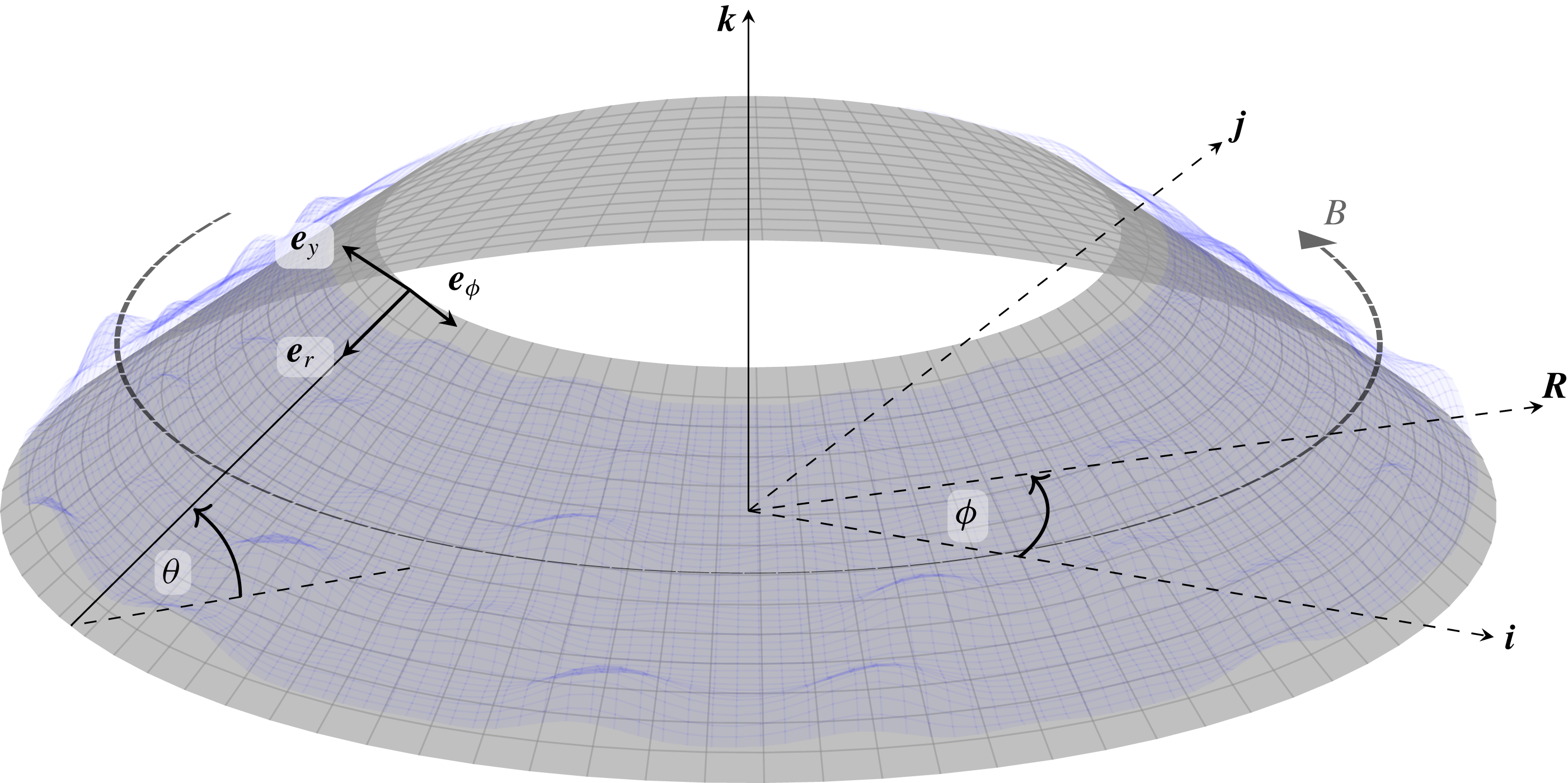
Schematic of the truncated conical divertor and free surface in the presence of a toroidal applied field
 $\boldsymbol{B}$
. The Cartesian coordinate basis is
 $(\boldsymbol{i},\boldsymbol{j},\boldsymbol{k})$
, the cylindrical coordinate basis is
 $(\boldsymbol{R},\boldsymbol{e}_{\unicode[STIX]{x1D719}},\boldsymbol{k})$
and the local divertor coordinate basis is
 $(\boldsymbol{e}_{r},\boldsymbol{e}_{y},\boldsymbol{e}_{\unicode[STIX]{x1D719}})$
. The inclination angle of the divertor to the horizontal is
 $\unicode[STIX]{x1D703}$
. Dashed lines lie in the same horizontal plane.

In the present paper, a genuinely axisymmetric geometry is considered, with a toroidal magnetic field that satisfies Maxwell’s equations both inside and outside the flowing liquid metal. We allow for a conducting substrate and a non-zero magnetic susceptibility of the liquid metal: although the susceptibility is very small in practice, we find that it can give rise to a non-negligible magnetic pressure when the applied magnetic field is very strong. Furthermore, the inclusion of a small but non-zero magnetic susceptibility exposes an inconsistency in the boundary conditions when an artificial external magnetic field is imposed (as in Gao & Morley Reference Gao and Morley2002). Like Gao & Morley (Reference Gao and Morley2002), we find that the velocity profile becomes increasingly exotic as the film thickness increases, but we show that such behaviour corresponds to unphysical solution branches that we suggest could never be observed in practice.
Our paper thus aims to put the results of Gao & Morley (Reference Gao and Morley2002) on a firmer theoretical footing, while elucidating when they may lack validity or self-consistency. However, for non-zero Reynolds number, there is no fully developed unidirectional flow in an axisymmetric geometry, and on the face of it a linear stability analysis analogous to that in Gao & Morley (Reference Gao and Morley2002) is not possible. Instead, we perform a multiple-scale stability analysis of high-frequency disturbances in which inertial effects may be significant despite the assumed smallness of the reduced Reynolds number. This approach results in an Orr–Summerfeld-type problem analogous to that obtained in Gao & Morley (Reference Gao and Morley2002), which we solve both asymptotically and numerically without introducing any artificial approximations. We find that the coupling between the magnetic induction and the flow may have a profound effect on the stability; in particular, there are regions of parameter space where the long-wave hydrodynamic instability identified by Yih (Reference Yih1963) is suppressed, resulting in a dramatic increase in the critical Reynolds number beyond which the base flow is unstable.
The paper is organised as follows. In § 2 we present the equations and boundary conditions governing the flow of the liquid metal down a conical divertor in the presence of a strong magnetic field. We then consider the leading-order system in the physically relevant limit in which the liquid film is thin compared to the length of the divertor substrate, and the induced field is much smaller than the applied field. Provided the reduced Reynolds number is small enough for inertia effects to be negligible, these assumptions allow us to obtain closed-form solutions for the velocity components and the induced field. Steady and unsteady solutions of the resulting thin-film equation for the film thickness are presented in § 3. In § 4 we analyse the stability of the free-surface flow in the presence of high-frequency inertial perturbations. We conclude § 4 with a detailed description of the important physical implications of the stability analysis. Finally, in § 5 we summarise and discuss our findings.
2 Model derivation
2.1 Governing equations and boundary conditions
2.1.1 Coordinate system
We consider the axisymmetric geometry sketched in figure 1. The liquid metal flows on a conical substrate inclined at an angle
 $\unicode[STIX]{x1D703}$
to the horizontal, and is subject to a magnetic field
 $\boldsymbol{B}$
which acts purely in the azimuthal direction. We define coordinates
 $(r,y,\unicode[STIX]{x1D719})$
that lie parallel and normal to the substrate as follows:
 $$\begin{eqnarray}\displaystyle \boldsymbol{r}(r,y,\unicode[STIX]{x1D719})=(r\cos \unicode[STIX]{x1D703}+y\sin \unicode[STIX]{x1D703})(\boldsymbol{i}\cos \unicode[STIX]{x1D719}+\boldsymbol{j}\sin \unicode[STIX]{x1D719})+(y\cos \unicode[STIX]{x1D703}-r\sin \unicode[STIX]{x1D703})\boldsymbol{k}, & & \displaystyle\end{eqnarray}$$
where
 $(\boldsymbol{i},\boldsymbol{j},\boldsymbol{k})$
is the usual Cartesian coordinate basis. The coordinates
 $(r,y,\unicode[STIX]{x1D719})$
are orthogonal, with scale factors given by
 $$\begin{eqnarray}\displaystyle \left|\frac{\unicode[STIX]{x2202}\boldsymbol{r}}{\unicode[STIX]{x2202}r}\right|=1,\quad \left|\frac{\unicode[STIX]{x2202}\boldsymbol{r}}{\unicode[STIX]{x2202}y}\right|=1,\quad \left|\frac{\unicode[STIX]{x2202}\boldsymbol{r}}{\unicode[STIX]{x2202}\unicode[STIX]{x1D719}}\right|=R, & & \displaystyle\end{eqnarray}$$
where the distance from the central axis is denoted by
 $$\begin{eqnarray}\displaystyle R=r\cos \unicode[STIX]{x1D703}+y\sin \unicode[STIX]{x1D703}>0. & & \displaystyle\end{eqnarray}$$
It is therefore straightforward to express the governing equations using the standard formulae for orthogonal curvilinear coordinates (see, for example, Weber & Arfken Reference Weber and Arfken2004, chap. 2).
2.1.2 Electromagnetic problem
The magnetic flux density
 $\boldsymbol{B}$
, electric field
 $\boldsymbol{E}$
and current
 $\boldsymbol{J}$
in a liquid metal flowing with velocity
 $\boldsymbol{u}$
satisfy the pre-Maxwell equations, with negligible displacement current, and Ohm’s law, namely
 $$\begin{eqnarray}\displaystyle \unicode[STIX]{x1D735}\boldsymbol{\cdot }\boldsymbol{B}=0,\quad \unicode[STIX]{x1D735}\times \boldsymbol{B}=\unicode[STIX]{x1D707}\boldsymbol{J}=\unicode[STIX]{x1D707}\unicode[STIX]{x1D70E}(\boldsymbol{E}+\boldsymbol{u}\times \boldsymbol{B}),\quad \frac{\unicode[STIX]{x2202}\boldsymbol{B}}{\unicode[STIX]{x2202}t}=-\unicode[STIX]{x1D735}\times \boldsymbol{E}, & & \displaystyle\end{eqnarray}$$
where
 $\unicode[STIX]{x1D70E}$
and
 $\unicode[STIX]{x1D707}$
denote conductivity and magnetic permeability, respectively. Elimination of
 $\boldsymbol{E}$
from (2.4) reveals that
 $\boldsymbol{B}$
satisfies the induction equation
 $$\begin{eqnarray}\displaystyle \frac{\unicode[STIX]{x2202}\boldsymbol{B}}{\unicode[STIX]{x2202}t}-\unicode[STIX]{x1D702}\unicode[STIX]{x1D6FB}^{2}\boldsymbol{B}=\unicode[STIX]{x1D735}\times (\boldsymbol{u}\times \boldsymbol{B}), & & \displaystyle\end{eqnarray}$$
where
 $\unicode[STIX]{x1D702}=1/(\unicode[STIX]{x1D707}\unicode[STIX]{x1D70E})$
is the magnetic diffusivity.
The formulation (2.5) removes the need to solve for the electric field or the current in the bulk, but we retain
 $\boldsymbol{E}$
and
 $\boldsymbol{J}$
for the moment while writing down the relevant boundary conditions. In our problem there are three interfaces: between the substrate and the space below, between the substrate and the liquid metal and between the liquid and the space above. At each such interface, we must impose continuity of the normal components of the magnetic flux density and the current, and the tangential components of the magnetic and electric fields, i.e.
 $$\begin{eqnarray}\displaystyle [\boldsymbol{n}\boldsymbol{\cdot }\boldsymbol{B}]_{-}^{+}=0,\quad [\boldsymbol{n}\boldsymbol{\cdot }\boldsymbol{J}]_{-}^{+}=0,\quad \left[\frac{1}{\unicode[STIX]{x1D707}}\boldsymbol{n}\times \boldsymbol{B}\right]_{-}^{+}=\mathbf{0},\quad [\boldsymbol{n}\times \boldsymbol{E}]_{-}^{+}=\mathbf{0}, & & \displaystyle\end{eqnarray}$$
where
 $\boldsymbol{n}$
is the unit normal to the interface. There is some redundancy in (2.6) when self-consistent forms are used for
 $\boldsymbol{B}$
,
 $\boldsymbol{J}$
and
 $\boldsymbol{E}$
. However, we retain all four boundary conditions for the moment to expose the inconsistency that occurs if one artificially imposes an external magnetic field that does not satisfy Maxwell’s equations.
2.1.3 Fluid dynamics
The velocity
 $\boldsymbol{u}(\boldsymbol{r},t)$
and the pressure
 $p(\boldsymbol{r},t)$
in the liquid satisfy the incompressible Navier–Stokes equations with body force terms due to the gravitational acceleration
 $-g\boldsymbol{k}$
and the Lorenz force, i.e.
 $$\begin{eqnarray}\displaystyle & \displaystyle \unicode[STIX]{x1D735}\boldsymbol{\cdot }\boldsymbol{u}=0, & \displaystyle\end{eqnarray}$$
 $$\begin{eqnarray}\displaystyle & \displaystyle \unicode[STIX]{x1D70C}\left(\frac{\unicode[STIX]{x2202}\boldsymbol{u}}{\unicode[STIX]{x2202}t}+(\boldsymbol{u}\boldsymbol{\cdot }\unicode[STIX]{x1D735})\boldsymbol{u}\right)=-\unicode[STIX]{x1D735}p+\unicode[STIX]{x1D70C}\unicode[STIX]{x1D708}\unicode[STIX]{x1D6FB}^{2}\boldsymbol{u}-\unicode[STIX]{x1D70C}g\boldsymbol{k}+\boldsymbol{J}\times \boldsymbol{B}, & \displaystyle\end{eqnarray}$$
 $\unicode[STIX]{x1D70C}$
and
 $\unicode[STIX]{x1D708}$
denote the density and kinematic viscosity of the liquid.
At the fluid–substrate boundary
 $y=0$
, we impose the no-slip boundary condition
 $\boldsymbol{u}=\mathbf{0}$
. At the free surface
 $y=h(r,\unicode[STIX]{x1D719},t)$
of the fluid, we have the usual kinematic and dynamic boundary conditions, but with an additional surface traction due to the Maxwell stress, i.e.
 $$\begin{eqnarray}\displaystyle \frac{\unicode[STIX]{x2202}h}{\unicode[STIX]{x2202}t}+\boldsymbol{u}\boldsymbol{\cdot }\unicode[STIX]{x1D735}(h-y)=0,\quad \left[\unicode[STIX]{x1D749}\boldsymbol{\cdot }\boldsymbol{n}+\frac{(\boldsymbol{B}\boldsymbol{\cdot }\boldsymbol{n})\boldsymbol{B}}{\unicode[STIX]{x1D707}}-\frac{|\boldsymbol{B}|^{2}\boldsymbol{n}}{2\unicode[STIX]{x1D707}}\right]_{-}^{+}=\unicode[STIX]{x1D6FE}\unicode[STIX]{x1D718}\boldsymbol{n}, & & \displaystyle\end{eqnarray}$$
where
 $\unicode[STIX]{x1D6FE}$
is the surface tension,
 $\unicode[STIX]{x1D718}=\unicode[STIX]{x1D735}\boldsymbol{\cdot }\boldsymbol{n}$
is the curvature of the surface and
 $$\begin{eqnarray}\displaystyle \unicode[STIX]{x1D749}=-p\boldsymbol{I}+\unicode[STIX]{x1D70C}\unicode[STIX]{x1D708}(\unicode[STIX]{x1D735}\boldsymbol{u}+\unicode[STIX]{x1D735}\boldsymbol{u}^{\text{T}}) & & \displaystyle\end{eqnarray}$$
is the viscous stress tensor.
2.1.4 Axisymmetric solution structure
We consider axisymmetric flow, with the velocity and pressure given by
 $$\begin{eqnarray}\displaystyle \boldsymbol{u}=u(r,y,t)\boldsymbol{e}_{r}+v(r,y,t)\boldsymbol{e}_{y},\quad p=p(r,y,t). & & \displaystyle\end{eqnarray}$$
We similarly assume that the free surface of the liquid is axisymmetric. The thickness of the liquid-metal film and of the underlying substrate are denoted by
 $h(r,t)$
and
 $h^{s}$
, respectively; thus the upper surface of the liquid and the lower surface of the substrate are given by
 $y=h(r,t)$
and
 $y=-h^{s}$
, respectively.
We note that, given the assumed symmetry of the geometry, both the induction equation (2.5) and the magnetic boundary conditions (2.6a,c
) are homogeneous in the
 $\boldsymbol{e}r$
- and
 $\boldsymbol{e}_{y}$
-directions. It follows that a purely toroidal applied field (parallel to
 $\boldsymbol{e}_{\unicode[STIX]{x1D719}}$
) induces a purely toroidal field, and we therefore restrict our attention henceforth to magnetic fields of the form
 $$\begin{eqnarray}\displaystyle \boldsymbol{B}=B(r,y,t)\boldsymbol{e}_{\unicode[STIX]{x1D719}}. & & \displaystyle\end{eqnarray}$$
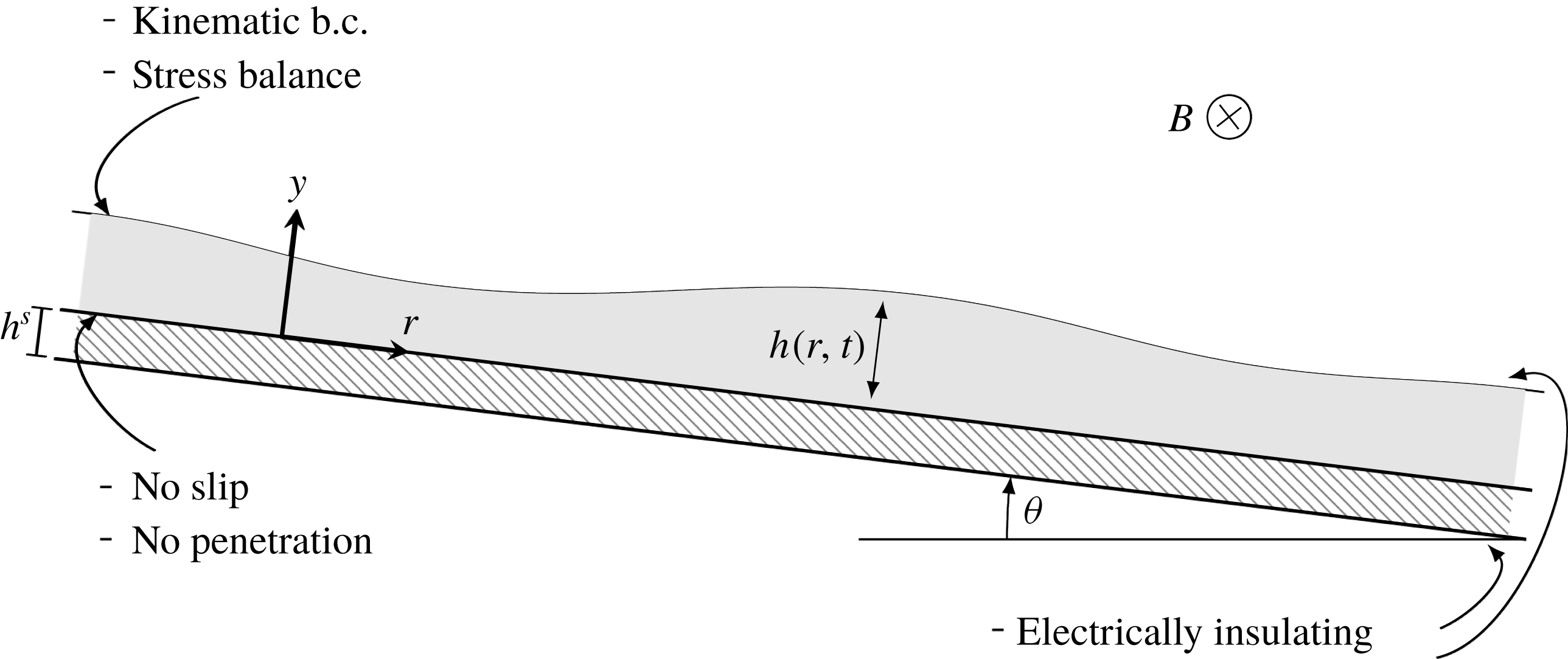
The corresponding two-dimensional configuration is sketched in figure 2.
Schematic of the effectively two-dimensional flow configuration.

Next we will spell out in detail how the governing equations and boundary conditions (2.5)–(2.8) simplify in each region and on each interface in the problem.
2.1.5 Vacuum
In
 $y<-h^{s}$
and
 $y>h(r,t)$
, we assume there is effectively free space, in which Maxwell’s equations (2.4) reduce to
 $\unicode[STIX]{x1D735}\boldsymbol{\cdot }\boldsymbol{B}=0$
and
 $\unicode[STIX]{x1D735}\times \boldsymbol{B}=\mathbf{0}$
, which can only be satisfied by a magnetic flux density proportional to
 $1/R$
, where
 $R$
is defined by (2.3). We therefore set the external field to be
 $$\begin{eqnarray}\displaystyle B=B^{a}(r,y)=\frac{B_{0}L}{R}=\frac{B_{0}L}{r\cos \unicode[STIX]{x1D703}+y\sin \unicode[STIX]{x1D703}}, & & \displaystyle\end{eqnarray}$$
where
 $L$
is a length scale and
 $B_{0}$
is a parameter measuring the field strength; in principle
 $B_{0}$
could be a function of time, but we will take it to be constant. The ‘applied field’
 $B^{a}$
is assumed to be given and, in practice, is generated by electromagnets some distance from the divertor.
2.1.6 Liquid
In
 $0<y<h(r,t)$
, we seek solutions with axisymmetric velocity and magnetic flux density given by (2.10) and (2.11). It is also helpful to decompose the magnetic flux density according to
 $$\begin{eqnarray}\displaystyle B=(1+\unicode[STIX]{x1D712})B^{a}+B^{i}, & & \displaystyle\end{eqnarray}$$
where
 $B^{a}$
is again the known applied field, given by (2.12), and
 $\unicode[STIX]{x1D712}$
is the magnetic susceptibility of the liquid. By substitution into (2.5), we find that the ‘induced field’
 $B^{i}$
in the liquid satisfies the equation
 $$\begin{eqnarray}\displaystyle & & \displaystyle \frac{\unicode[STIX]{x2202}B^{i}}{\unicode[STIX]{x2202}t}-\unicode[STIX]{x1D702}\left[\frac{\unicode[STIX]{x2202}}{\unicode[STIX]{x2202}r}\left(\frac{1}{R}\frac{\unicode[STIX]{x2202}}{\unicode[STIX]{x2202}r}(RB^{i})\right)+\frac{\unicode[STIX]{x2202}}{\unicode[STIX]{x2202}y}\left(\frac{1}{R}\frac{\unicode[STIX]{x2202}}{\unicode[STIX]{x2202}y}(RB^{i})\right)\right]\nonumber\\ \displaystyle & & \displaystyle \quad =-Ru\frac{\unicode[STIX]{x2202}}{\unicode[STIX]{x2202}r}\left[\frac{(1+\unicode[STIX]{x1D712})B^{a}+B^{i}}{R}\right]-Rv\frac{\unicode[STIX]{x2202}}{\unicode[STIX]{x2202}y}\left[\frac{(1+\unicode[STIX]{x1D712})B^{a}+B^{i}}{R}\right],\end{eqnarray}$$
where
 $\unicode[STIX]{x1D702}$
is the magnetic diffusivity of the liquid metal.
Next we write out the Navier–Stokes equations (2.7) with respect to our orthogonal coordinate system, namely
 $$\begin{eqnarray}\displaystyle \frac{\unicode[STIX]{x2202}}{\unicode[STIX]{x2202}r}(Ru)+\frac{\unicode[STIX]{x2202}}{\unicode[STIX]{x2202}y}(Rv) & =0, & \displaystyle\end{eqnarray}$$
 $$\begin{eqnarray}\displaystyle \unicode[STIX]{x1D70C}\left(\frac{\unicode[STIX]{x2202}u}{\unicode[STIX]{x2202}t}+u\frac{\unicode[STIX]{x2202}u}{\unicode[STIX]{x2202}r}+v\frac{\unicode[STIX]{x2202}u}{\unicode[STIX]{x2202}y}\right) & = & \displaystyle -\frac{\unicode[STIX]{x2202}p}{\unicode[STIX]{x2202}r}+\frac{\unicode[STIX]{x1D70C}\unicode[STIX]{x1D708}}{R}\left[\frac{\unicode[STIX]{x2202}^{2}}{\unicode[STIX]{x2202}r^{2}}(Ru)+\frac{\unicode[STIX]{x2202}}{\unicode[STIX]{x2202}y}\left(R\frac{\unicode[STIX]{x2202}u}{\unicode[STIX]{x2202}y}+v\frac{\unicode[STIX]{x2202}R}{\unicode[STIX]{x2202}r}\right)\right]\nonumber\\ \displaystyle & & \displaystyle +\,\unicode[STIX]{x1D70C}g\sin \unicode[STIX]{x1D703}-\frac{(1+\unicode[STIX]{x1D712})B^{a}+B^{i}}{(1+\unicode[STIX]{x1D712})\unicode[STIX]{x1D707}_{0}R}\frac{\unicode[STIX]{x2202}}{\unicode[STIX]{x2202}r}(RB^{i}),\end{eqnarray}$$
 $$\begin{eqnarray}\displaystyle \unicode[STIX]{x1D70C}\left(\frac{\unicode[STIX]{x2202}v}{\unicode[STIX]{x2202}t}+u\frac{\unicode[STIX]{x2202}v}{\unicode[STIX]{x2202}r}+v\frac{\unicode[STIX]{x2202}v}{\unicode[STIX]{x2202}y}\right) & = & \displaystyle -\frac{\unicode[STIX]{x2202}p}{\unicode[STIX]{x2202}y}+\frac{\unicode[STIX]{x1D70C}\unicode[STIX]{x1D708}}{R}\left[\frac{\unicode[STIX]{x2202}^{2}}{\unicode[STIX]{x2202}y^{2}}(Rv)+\frac{\unicode[STIX]{x2202}}{\unicode[STIX]{x2202}r}\left(R\frac{\unicode[STIX]{x2202}v}{\unicode[STIX]{x2202}r}+u\frac{\unicode[STIX]{x2202}R}{\unicode[STIX]{x2202}y}\right)\right]\nonumber\\ \displaystyle & & \displaystyle -\,\unicode[STIX]{x1D70C}g\cos \unicode[STIX]{x1D703}-\frac{(1+\unicode[STIX]{x1D712})B^{a}+B^{i}}{(1+\unicode[STIX]{x1D712})\unicode[STIX]{x1D707}_{0}R}\frac{\unicode[STIX]{x2202}}{\unicode[STIX]{x2202}y}(RB^{i}).\end{eqnarray}$$
 $\unicode[STIX]{x1D707}=\unicode[STIX]{x1D707}_{0}(1+\unicode[STIX]{x1D712})$
, where
 $\unicode[STIX]{x1D707}_{0}$
is the permeability of free space.
2.1.7 Substrate
In
 $-h^{s}<y<0$
, the magnetic flux density satisfies the induction equation (2.5) with
 $\boldsymbol{u}=\mathbf{0}$
and
 $\unicode[STIX]{x1D702}=\unicode[STIX]{x1D702}^{s}$
, the magnetic diffusivity of the substrate. We substitute for
 $\boldsymbol{B}$
from (2.11) and again decompose the toroidal magnetic flux component as follows:
 $$\begin{eqnarray}\displaystyle B=(1+\unicode[STIX]{x1D712}^{s})B^{a}+B^{is}, & & \displaystyle\end{eqnarray}$$
where
 $\unicode[STIX]{x1D712}^{s}$
is the magnetic susceptibility of the substrate. It then follows from (2.5) that the induced field
 $B^{is}$
in the substrate satisfies the equation
 $$\begin{eqnarray}\displaystyle \frac{\unicode[STIX]{x2202}B^{is}}{\unicode[STIX]{x2202}t}=\unicode[STIX]{x1D702}^{s}\left[\frac{\unicode[STIX]{x2202}}{\unicode[STIX]{x2202}r}\left(\frac{1}{R}\frac{\unicode[STIX]{x2202}}{\unicode[STIX]{x2202}r}(RB^{is})\right)+\frac{\unicode[STIX]{x2202}}{\unicode[STIX]{x2202}y}\left(\frac{1}{R}\frac{\unicode[STIX]{x2202}}{\unicode[STIX]{x2202}y}(RB^{is})\right)\right]. & & \displaystyle\end{eqnarray}$$
2.1.8 Fluid–vacuum
Next we apply the boundary conditions (2.6) and (2.8) at the free surface
 $y=h(r,t)$
of the fluid. Given the axisymmetric geometry and purely toroidal magnetic field, the first magnetic boundary condition (2.6a
) is satisfied identically, and the next two conditions (2.6b,c
) are both equivalent to
 $$\begin{eqnarray}\displaystyle \left[\frac{B}{\unicode[STIX]{x1D707}}\right]_{-}^{+}=0. & & \displaystyle\end{eqnarray}$$
Upon decomposing the magnetic flux density according to (2.13), we find that (2.18) reduces to the condition
 $$\begin{eqnarray}\displaystyle B^{i}=0\quad \text{at }y=h(r,t) & & \displaystyle\end{eqnarray}$$
on the induced field at the free surface. The final electromagnetic jump condition (2.6d
) provides an effective boundary condition for the electric field
 $\boldsymbol{E}$
in the vacuum above the liquid, should one wish to calculate it.
We note here in passing that the ad hoc approach adopted by Gao & Morley (Reference Gao and Morley2002) introduces spurious currents in the vacuum region
 $y>h(r,t)$
and gives rise to an irreconcilable inconsistency between the four electromagnetic boundary conditions (2.6), except in the special case where the magnetic susceptibility
 $\unicode[STIX]{x1D712}$
of the fluid is zero.
In component form, the fluid dynamic boundary conditions (2.8) at the free surface
 $y=h(r,t)$
read
 $$\begin{eqnarray}\displaystyle & \displaystyle v=\frac{\unicode[STIX]{x2202}h}{\unicode[STIX]{x2202}t}+u\frac{\unicode[STIX]{x2202}h}{\unicode[STIX]{x2202}r}. & \displaystyle\end{eqnarray}$$
 $$\begin{eqnarray}\displaystyle & \displaystyle \left[1-\left(\frac{\unicode[STIX]{x2202}h}{\unicode[STIX]{x2202}r}\right)^{2}\right]\left[\frac{\unicode[STIX]{x2202}u}{\unicode[STIX]{x2202}y}+\frac{\unicode[STIX]{x2202}v}{\unicode[STIX]{x2202}r}\right]+2\frac{\unicode[STIX]{x2202}h}{\unicode[STIX]{x2202}r}\left[\frac{\unicode[STIX]{x2202}v}{\unicode[STIX]{x2202}y}-\frac{\unicode[STIX]{x2202}u}{\unicode[STIX]{x2202}r}\right]=0, & \displaystyle\end{eqnarray}$$
 $$\begin{eqnarray}\displaystyle & \displaystyle -p+2\unicode[STIX]{x1D70C}\unicode[STIX]{x1D708}\left[1+\left(\frac{\unicode[STIX]{x2202}h}{\unicode[STIX]{x2202}r}\right)^{2}\right]^{-1}\left[\frac{\unicode[STIX]{x2202}v}{\unicode[STIX]{x2202}y}-2\frac{\unicode[STIX]{x2202}h}{\unicode[STIX]{x2202}r}\left(\frac{\unicode[STIX]{x2202}u}{\unicode[STIX]{x2202}y}+\frac{\unicode[STIX]{x2202}v}{\unicode[STIX]{x2202}r}\right)+\left(\frac{\unicode[STIX]{x2202}h}{\unicode[STIX]{x2202}r}\right)^{2}\frac{\unicode[STIX]{x2202}u}{\unicode[STIX]{x2202}r}\right]=\unicode[STIX]{x1D6FE}\unicode[STIX]{x1D718}+\frac{\unicode[STIX]{x1D712}{B^{a}}^{2}}{2\unicode[STIX]{x1D707}_{0}}, & \displaystyle \nonumber\\ \displaystyle & & \displaystyle\end{eqnarray}$$
 $$\begin{eqnarray}\displaystyle \unicode[STIX]{x1D718}=\left[1+\left(\frac{\unicode[STIX]{x2202}h}{\unicode[STIX]{x2202}r}\right)^{2}\right]^{-3/2}\frac{\unicode[STIX]{x2202}^{2}h}{\unicode[STIX]{x2202}r^{2}}+\frac{1}{R}\left[1+\left(\frac{\unicode[STIX]{x2202}h}{\unicode[STIX]{x2202}r}\right)^{2}\right]^{-1/2}\left(\cos \unicode[STIX]{x1D703}\frac{\unicode[STIX]{x2202}h}{\unicode[STIX]{x2202}r}-\sin \unicode[STIX]{x1D703}\right). & & \displaystyle\end{eqnarray}$$
2.1.9 Substrate–fluid
At
 $y=0$
, the current continuity condition in (2.6) is again satisfied identically, and the remaining independent conditions for the magnetic flux density are
 $$\begin{eqnarray}\displaystyle \frac{B^{is}}{1+\unicode[STIX]{x1D712}^{s}}=\frac{B^{i}}{1+\unicode[STIX]{x1D712}},\quad \unicode[STIX]{x1D702}^{s}\frac{\unicode[STIX]{x2202}}{\unicode[STIX]{x2202}y}(RB^{is})=\unicode[STIX]{x1D702}\frac{\unicode[STIX]{x2202}}{\unicode[STIX]{x2202}y}(RB^{i}), & & \displaystyle\end{eqnarray}$$
while the velocity satisfies the no-slip condition
 $$\begin{eqnarray}\displaystyle u=v=0. & & \displaystyle\end{eqnarray}$$
2.1.10 Substrate–vacuum
Finally, at the boundary
 $y=-h^{s}$
between the substrate and the vacuum below, the boundary conditions (2.6a–c
) all collapse to
 $$\begin{eqnarray}\displaystyle B^{is}=0. & & \displaystyle\end{eqnarray}$$
As in § 2.1.8, the final condition (2.6d ) just provides a boundary condition for the electric field in the space below the substrate, should one wish to solve for it.
2.2 Leading-order dimensionless model
We now non-dimensionalise the equations and boundary conditions set out in § 2.1 and then exploit the sizes of the relevant dimensionless parameters to simplify the resulting model. We denote typical length and thickness scales for the film by
 $L$
and
 ${\mathcal{H}}$
, respectively, and assume that the aspect ratio
 $\unicode[STIX]{x1D716}={\mathcal{H}}/L$
is small. By balancing viscous stress with gravity in (2.15c
), we infer a suitable velocity scale
 $$\begin{eqnarray}\displaystyle U=\frac{{\mathcal{H}}^{2}g\sin \unicode[STIX]{x1D703}}{\unicode[STIX]{x1D708}}. & & \displaystyle\end{eqnarray}$$
The variables are then non-dimensionalised as follows:
 $$\begin{eqnarray}\displaystyle r=Lr^{\prime },\quad y={\mathcal{H}}y^{\prime },\quad h={\mathcal{H}}h^{\prime },\quad t=(L/U)t^{\prime }, & & \displaystyle\end{eqnarray}$$
 $$\begin{eqnarray}\displaystyle u=Uu^{\prime },\quad v=\unicode[STIX]{x1D716}Uv^{\prime },\quad p=\unicode[STIX]{x1D70C}gL\sin \unicode[STIX]{x1D703}p^{\prime },\quad B^{i}=\frac{2\unicode[STIX]{x1D716}^{2}(1+\unicode[STIX]{x1D712})B_{0}LU}{\unicode[STIX]{x1D702}\cos \unicode[STIX]{x1D703}}B^{i^{\prime }},\quad & & \displaystyle\end{eqnarray}$$
before dropping the primes to reduce clutter.
The relevant dimensionless parameters are:
 $$\begin{eqnarray}\displaystyle & \displaystyle \text{aspect ratio}\quad \unicode[STIX]{x1D716}=\frac{{\mathcal{H}}}{L}=O(10^{-4}), & \displaystyle\end{eqnarray}$$
 $$\begin{eqnarray}\displaystyle & \displaystyle \text{Reynolds number}\quad Re=\frac{U{\mathcal{H}}}{\unicode[STIX]{x1D708}}=\frac{g{\mathcal{H}}^{3}\sin \unicode[STIX]{x1D703}}{\unicode[STIX]{x1D708}^{2}}=O(1), & \displaystyle\end{eqnarray}$$
 $$\begin{eqnarray}\displaystyle & \displaystyle \text{Hartmann number}\quad Ha=B_{0}{\mathcal{H}}\sqrt{\frac{\unicode[STIX]{x1D70E}}{\unicode[STIX]{x1D70C}\unicode[STIX]{x1D708}}}=O(10), & \displaystyle\end{eqnarray}$$
 $$\begin{eqnarray}\displaystyle & \displaystyle \text{Bond number}\quad Bo=\frac{\unicode[STIX]{x1D70C}g{\mathcal{H}}^{2}\sin \unicode[STIX]{x1D703}}{\unicode[STIX]{x1D6FE}}=O(10^{-5}), & \displaystyle\end{eqnarray}$$
 $$\begin{eqnarray}\displaystyle & \displaystyle \text{magnetic Reynolds number}\quad Rm=\frac{U{\mathcal{H}}}{\unicode[STIX]{x1D702}}=\frac{g{\mathcal{H}}^{3}\sin \unicode[STIX]{x1D703}}{\unicode[STIX]{x1D708}\unicode[STIX]{x1D702}}=O(10^{-5}). & \displaystyle\end{eqnarray}$$
 $L=1~\text{m}$
and film thickness
 ${\mathcal{H}}=0.1~\text{mm}$
, based on calculations from the fusion literature (Ono et al.
Reference Ono, Majeski, Jaworski, Hirooka, Kaita, Gray, Maingi, Skinner, Christenson and Ruzic2017) that have been established experimentally (Platacis et al.
Reference Platacis, Flerov, Klukin, Ivanov, Sobolevs, Shishko, Zaharov and Gryaznevich2014). We also take a typical inclination angle
 $\unicode[STIX]{x1D703}=0.1$
radians and applied magnetic field strength
 $B_{0}=1~\text{T}$
. For the moment, we neglect terms of order
 $\unicode[STIX]{x1D716}^{2}$
and
 $\unicode[STIX]{x1D716}Rm$
(both of which are certainly very small) to get a leading-order lubrication model.
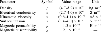
Material properties of liquid lithium in the temperature range
 $180{-}600\,^{\circ }\text{C}$
(taken from Davison Reference Davison1968; Shimokawa, Itami & Shimoji Reference Shimokawa, Itami and Shimoji1986).

The magnetic field in the substrate satisfies the leading-order version of (2.17), namely
 $$\begin{eqnarray}\displaystyle \frac{\unicode[STIX]{x2202}^{2}B^{is}}{\unicode[STIX]{x2202}y^{2}}=0, & & \displaystyle\end{eqnarray}$$
while the boundary conditions (2.22) and (2.24) reduce to
 $$\begin{eqnarray}\displaystyle B^{is}=0\quad \text{at }y=-h^{s}, & & \displaystyle\end{eqnarray}$$
 $$\begin{eqnarray}\displaystyle \frac{B^{is}}{1+\unicode[STIX]{x1D712}^{s}}=\frac{B^{i}}{1+\unicode[STIX]{x1D712}},\quad \unicode[STIX]{x1D702}^{s}\frac{\unicode[STIX]{x2202}B^{is}}{\unicode[STIX]{x2202}y}=\unicode[STIX]{x1D702}\frac{\unicode[STIX]{x2202}B^{i}}{\unicode[STIX]{x2202}y}\quad \text{at }y=0, & & \displaystyle\end{eqnarray}$$
where the substrate thickness
 $h^{s}$
has been normalised with the film thickness scaling
 ${\mathcal{H}}$
. By eliminating
 $B^{is}$
, we deduce that the magnetic field in the liquid satisfies the effective Robin boundary condition
 $$\begin{eqnarray}\displaystyle \frac{\unicode[STIX]{x2202}B^{i}}{\unicode[STIX]{x2202}y}=aB^{i}\quad \text{at }y=0, & & \displaystyle\end{eqnarray}$$
where
 $$\begin{eqnarray}\displaystyle a=\frac{\unicode[STIX]{x1D70E}}{h^{s}\unicode[STIX]{x1D70E}^{s}}. & & \displaystyle\end{eqnarray}$$
The dimensionless parameter
 $a$
allows us to interpolate between the extreme cases of a perfectly insulating substrate (
 $a\rightarrow \infty$
) and a perfectly conducting substrate (
 $a\rightarrow 0$
).
When terms of order
 $\unicode[STIX]{x1D716}^{2}$
,
 $\unicode[STIX]{x1D716}Rm$
and
 $\unicode[STIX]{x1D716}^{3}Ha^{2}Rm$
are neglected, the
 $r$
-component (2.15b
) of the momentum equation in the fluid layer reduces to
 $$\begin{eqnarray}\displaystyle \unicode[STIX]{x1D716}Re\left(\frac{\unicode[STIX]{x2202}u}{\unicode[STIX]{x2202}t}+u\frac{\unicode[STIX]{x2202}u}{\unicode[STIX]{x2202}r}+v\frac{\unicode[STIX]{x2202}u}{\unicode[STIX]{x2202}y}\right)=-\frac{\unicode[STIX]{x2202}p}{\unicode[STIX]{x2202}r}+1+\frac{\unicode[STIX]{x2202}^{2}u}{\unicode[STIX]{x2202}y^{2}}-\frac{2\unicode[STIX]{x1D716}^{2}(1+\unicode[STIX]{x1D712})^{2}Ha^{2}}{\cos ^{2}\unicode[STIX]{x1D703}}\frac{1}{r^{2}}\frac{\unicode[STIX]{x2202}}{\unicode[STIX]{x2202}r}(rB^{i}).\quad & & \displaystyle\end{eqnarray}$$
Similarly, neglecting terms of order
 $\unicode[STIX]{x1D716}^{2}$
,
 $\unicode[STIX]{x1D716}^{3}Re$
,
 $\unicode[STIX]{x1D716}Rm$
and
 $\unicode[STIX]{x1D716}^{3}Ha^{2}Rm$
in the
 $y$
-component (2.15c
) of the momentum equation, we obtain
 $$\begin{eqnarray}\displaystyle \frac{\unicode[STIX]{x2202}p}{\unicode[STIX]{x2202}y}=-\unicode[STIX]{x1D716}\cot \unicode[STIX]{x1D703}-\frac{2\unicode[STIX]{x1D716}^{2}(1+\unicode[STIX]{x1D712})^{2}Ha^{2}}{\cos ^{2}\unicode[STIX]{x1D703}}\frac{1}{r}\frac{\unicode[STIX]{x2202}B_{i}}{\unicode[STIX]{x2202}y}. & & \displaystyle\end{eqnarray}$$
The normal stress boundary condition (2.20c ) reduces to
 $$\begin{eqnarray}\displaystyle p=-\frac{\unicode[STIX]{x1D716}^{3}}{Bo}\unicode[STIX]{x1D718}-\frac{\unicode[STIX]{x1D712}(1+\unicode[STIX]{x1D712})\unicode[STIX]{x1D716}Ha^{2}}{2Rm\cos ^{2}\unicode[STIX]{x1D703}}\frac{1}{r^{2}}\quad \text{at }y=h(r,t), & & \displaystyle\end{eqnarray}$$
where
 $$\begin{eqnarray}\displaystyle \unicode[STIX]{x1D718}=\frac{\unicode[STIX]{x2202}^{2}h}{\unicode[STIX]{x2202}r^{2}}+\frac{1}{r}\left(\frac{\unicode[STIX]{x2202}h}{\unicode[STIX]{x2202}r}-\frac{\tan \unicode[STIX]{x1D703}}{\unicode[STIX]{x1D716}}\right) & & \displaystyle\end{eqnarray}$$
is the dimensionless curvature of the free surface. The pressure within the fluid layer is thus found to be given by
 $$\begin{eqnarray}\displaystyle p=-\frac{\unicode[STIX]{x1D716}^{3}}{Bo}\unicode[STIX]{x1D718}-\frac{\unicode[STIX]{x1D712}(1+\unicode[STIX]{x1D712})\unicode[STIX]{x1D716}Ha^{2}}{2Rm\cos ^{2}\unicode[STIX]{x1D703}}\frac{1}{r^{2}}+\unicode[STIX]{x1D716}\cot \unicode[STIX]{x1D703}(h-y)-\frac{2\unicode[STIX]{x1D716}^{2}(1+\unicode[STIX]{x1D712})^{2}Ha^{2}}{\cos ^{2}\unicode[STIX]{x1D703}}\frac{B^{i}}{r}. & & \displaystyle\end{eqnarray}$$
The second term on the right-hand side of (2.32a
) arises from the component of gravity parallel to the substrate, and is here equal to
 $1$
in dimensionless terms due to the choice of the velocity scale (2.25). The same choice gives rise to the coefficient
 $\unicode[STIX]{x1D716}\cot \unicode[STIX]{x1D703}$
multiplying the third term on the right-hand side of (2.33c
), which represents the normalised coefficient of gravity perpendicular to the substrate.
In addition to
 $a$
, we identify the other combinations of dimensionless parameters that appear in the model as follows:
 $$\begin{eqnarray}\displaystyle & \displaystyle \text{reduced Reynolds number}\quad Re^{\ast }=\unicode[STIX]{x1D716}Re=O(10^{-4}), & \displaystyle\end{eqnarray}$$
 $$\begin{eqnarray}\displaystyle & \displaystyle \text{reduced Hartmann number}\quad \unicode[STIX]{x1D706}^{2}=\frac{\unicode[STIX]{x1D716}(1+\unicode[STIX]{x1D712})Ha}{\cos \unicode[STIX]{x1D703}}=O(10^{-1}), & \displaystyle\end{eqnarray}$$
 $$\begin{eqnarray}\displaystyle & \displaystyle \text{magnetic stress parameter}\quad \unicode[STIX]{x1D6FD}=\frac{\unicode[STIX]{x1D712}(1+\unicode[STIX]{x1D712})\unicode[STIX]{x1D716}Ha^{2}}{2Rm\cos ^{2}\unicode[STIX]{x1D703}}=O(10^{-2}), & \displaystyle\end{eqnarray}$$
 $$\begin{eqnarray}\displaystyle & \displaystyle \text{capillary parameter}\quad \unicode[STIX]{x1D6E4}=\frac{\unicode[STIX]{x1D716}^{3}}{Bo}=O(10^{-7}), & \displaystyle\end{eqnarray}$$
 $$\begin{eqnarray}\displaystyle & \displaystyle \text{geometrical parameter}\quad \unicode[STIX]{x1D6FC}=\unicode[STIX]{x1D716}\cot \unicode[STIX]{x1D703}=O(10^{-3}). & \displaystyle\end{eqnarray}$$
 $\unicode[STIX]{x1D706}^{2}$
and
 $\unicode[STIX]{x1D6FD}$
are proportional to
 $B_{0}$
and to
 $B_{0}^{2}$
, respectively, and so might become important at slightly higher applied magnetic field strengths. Both surface tension and the transverse component of gravity can act as regularising influences, so we will retain them in the model for the moment but neglect all except the highest derivative term in the curvature
 $\unicode[STIX]{x1D718}$
.
In the limit where
 $Re^{\ast }\rightarrow 0$
, our leading-order problem then reads
 $$\begin{eqnarray}\displaystyle & \displaystyle \frac{\unicode[STIX]{x2202}^{2}B^{i}}{\unicode[STIX]{x2202}y^{2}}=-\frac{u}{r^{2}}, & \displaystyle\end{eqnarray}$$
 $$\begin{eqnarray}\displaystyle & \displaystyle \frac{1}{r}\frac{\unicode[STIX]{x2202}}{\unicode[STIX]{x2202}r}(ru)+\frac{\unicode[STIX]{x2202}v}{\unicode[STIX]{x2202}y}=0, & \displaystyle\end{eqnarray}$$
 $$\begin{eqnarray}\displaystyle & \displaystyle -\frac{\unicode[STIX]{x2202}^{2}u}{\unicode[STIX]{x2202}y^{2}}+4\unicode[STIX]{x1D706}^{4}\frac{B^{i}}{r^{2}}=\unicode[STIX]{x1D711}(r,t):=1-\unicode[STIX]{x1D6FC}\frac{\unicode[STIX]{x2202}h}{\unicode[STIX]{x2202}r}-\frac{2\unicode[STIX]{x1D6FD}}{r^{3}}+\unicode[STIX]{x1D6E4}\frac{\unicode[STIX]{x2202}^{3}h}{\unicode[STIX]{x2202}r^{3}}, & \displaystyle\end{eqnarray}$$
 $$\begin{eqnarray}\displaystyle & \displaystyle u=v=\frac{\unicode[STIX]{x2202}B^{i}}{\unicode[STIX]{x2202}y}-aB^{i}=0\quad \text{at }y=0, & \displaystyle\end{eqnarray}$$
 $$\begin{eqnarray}\displaystyle & \displaystyle \frac{\unicode[STIX]{x2202}u}{\unicode[STIX]{x2202}y}=v-\frac{\unicode[STIX]{x2202}h}{\unicode[STIX]{x2202}t}-u\frac{\unicode[STIX]{x2202}h}{\unicode[STIX]{x2202}r}=B^{i}=0\quad \text{at }y=h(r,t). & \displaystyle\end{eqnarray}$$
 $\unicode[STIX]{x1D711}(r,t)$
defined in (2.35c
) represent, respectively, the effects of gravity parallel and normal to the substrate, the magnetic contribution to the pressure and surface tension. In particular,
 $\unicode[STIX]{x1D6FD}$
measures the effect on the flow due to a non-zero magnetic susceptibility
 $\unicode[STIX]{x1D712}$
in the liquid. Although
 $\unicode[STIX]{x1D712}$
is usually very small, since
 $\unicode[STIX]{x1D6FD}$
scales with
 $B_{0}^{2}$
, this effect may still be significant when the applied field is sufficiently strong. We note also that (provided
 $\unicode[STIX]{x1D712}>0$
), the magnetic pressure contribution always acts in opposition to the gravitational body force, and could even drive flow up the sloping substrate at large enough values of
 $\unicode[STIX]{x1D6FD}$
.
3 Thin film equation
3.1 Derivation and analysis
The problem (2.35) and (2.36) can readily be solved for
 $u$
,
 $v$
and
 $B^{i}$
. We normalise the problem by defining
 $$\begin{eqnarray}\displaystyle u(r,y,t)=\frac{\unicode[STIX]{x1D711}}{a^{2}\unicode[STIX]{x1D701}^{2}}{\mathcal{U}}(Y;H,\unicode[STIX]{x1D701}),\quad B^{i}(r,y,t)=\frac{\unicode[STIX]{x1D711}}{a^{4}\unicode[STIX]{x1D701}^{4}r^{2}}{\mathcal{B}}(Y;H,\unicode[STIX]{x1D701}), & & \displaystyle\end{eqnarray}$$
where
 $$\begin{eqnarray}\displaystyle Y=\frac{y}{h},\quad H=\frac{\unicode[STIX]{x1D706}h}{r},\quad \unicode[STIX]{x1D701}=\frac{\unicode[STIX]{x1D706}}{ar}. & & \displaystyle\end{eqnarray}$$
Then the governing equations (2.35) and boundary conditions (2.36) imply that
 ${\mathcal{U}}(Y)$
and
 ${\mathcal{B}}(Y)$
satisfy the problem
 $$\begin{eqnarray}\displaystyle & \displaystyle \frac{\text{d}^{2}{\mathcal{B}}}{\text{d}Y^{2}}+H^{2}{\mathcal{U}}=\frac{\text{d}^{2}{\mathcal{U}}}{\text{d}Y^{2}}-4H^{2}{\mathcal{B}}+H^{2}=0, & \displaystyle\end{eqnarray}$$
 $$\begin{eqnarray}\displaystyle & \displaystyle {\mathcal{U}}(0)=\frac{\text{d}{\mathcal{B}}}{\text{d}Y}(0)-\frac{H}{\unicode[STIX]{x1D701}}{\mathcal{B}}(0)=\frac{\text{d}{\mathcal{U}}}{\text{d}Y}(1)={\mathcal{B}}(1)=0, & \displaystyle\end{eqnarray}$$
 $Y$
for various values of the scaled thickness
 $H$
and the scaled field strength
 $\unicode[STIX]{x1D701}$
.
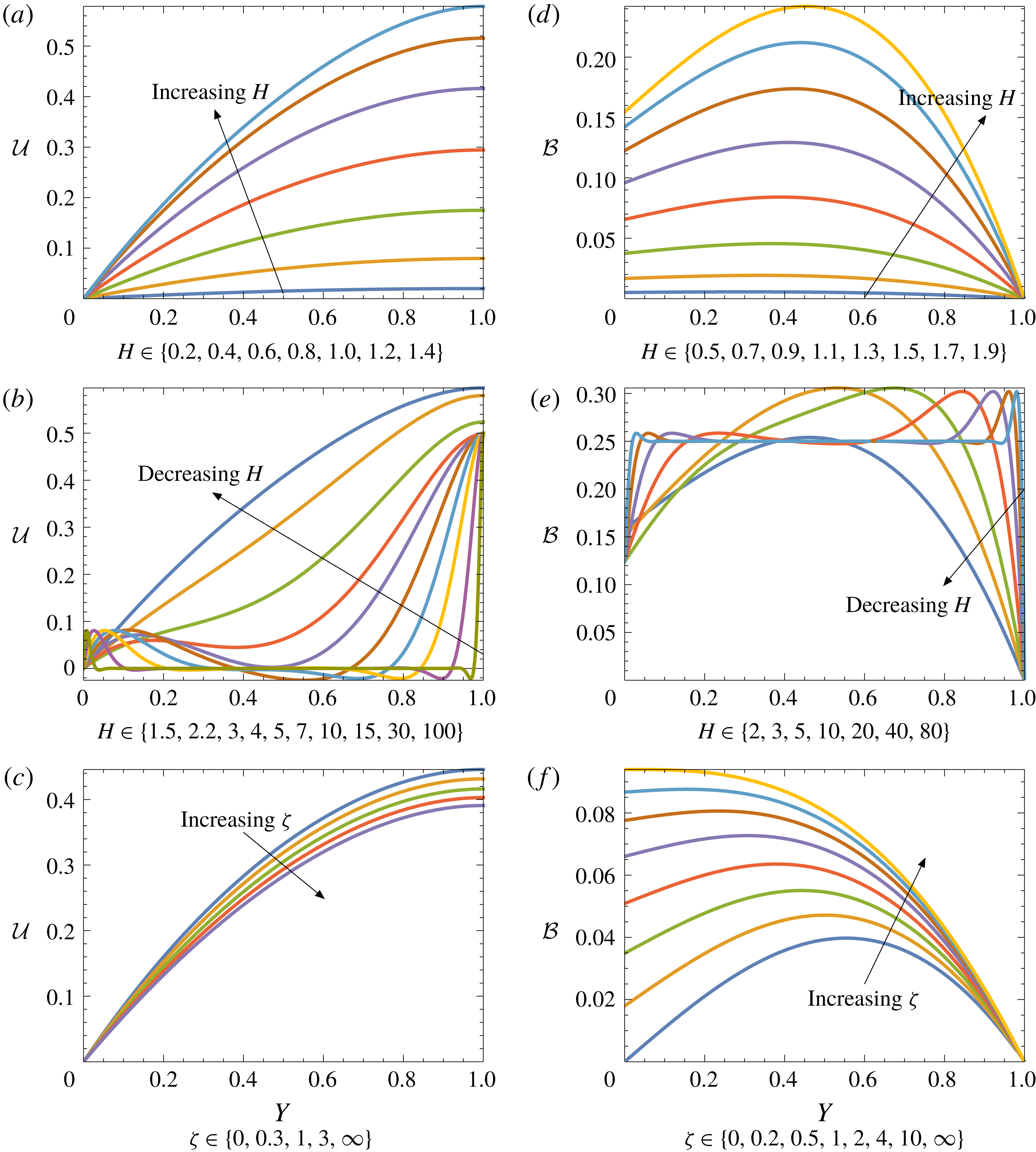
In figure 3(a,d) we observe that, for relatively small values of
 $H$
, the normalised magnetic field and velocity both increase with increasing
 $H$
; the induced field remains concave, with a global maximum in the interior of the film, and the velocity remains monotonic with respect to the vertical position
 $y$
. This behaviour is consistent with the classical parabolic hydrodynamic flow profile, which is recovered in the limit
 $H\rightarrow 0$
. For larger values of
 $H$
, as shown in figure 3(b), the velocity becomes non-monotonic and increasingly oscillatory, and for sufficiently large
 $H$
can even become negative within the film. Meanwhile, the induced field becomes approximately constant in the interior of the fluid, with magnetic forces balancing gravitational forces, while other effects manifest only in thin boundary layers, as shown in figure 3(e).
Figure 3(f) shows that the value of
 $\unicode[STIX]{x1D701}$
has a pronounced effect on the induced field. This behaviour reflects the boundary condition (3.3b
) that interpolates between a perfectly insulating substrate, with
 ${\mathcal{B}}(0)\rightarrow 0$
as
 $\unicode[STIX]{x1D701}\rightarrow 0$
, and a perfectly conducting substrate, with
 ${\mathcal{B}}^{\prime }(0)\rightarrow 0$
as
 $\unicode[STIX]{x1D701}\rightarrow \infty$
. However, with
 $H=1$
, the magnitude of the induced field remains rather small, and figure 3(c) shows that it has little influence on the velocity profile.
Scaled velocity
 ${\mathcal{U}}$
(a–c) and induced magnetic field
 ${\mathcal{B}}$
(d–f) plotted versus
 $Y=y/h$
. In (a,b,d,e) we fix
 $\unicode[STIX]{x1D701}=1$
and vary
 $H$
; in (c,f) we fix
 $H=1$
and vary
 $\unicode[STIX]{x1D701}$
.

Having solved for
 $u(r,y,t)$
, we integrate the mass conservation equation (2.35b
) and apply the kinematic boundary conditions at
 $y=0$
and
 $y=h$
to obtain an evolution equation for the film thickness in the form
 $$\begin{eqnarray}\displaystyle \frac{\unicode[STIX]{x2202}h}{\unicode[STIX]{x2202}t}+\frac{1}{r}\frac{\unicode[STIX]{x2202}}{\unicode[STIX]{x2202}r}(r\unicode[STIX]{x1D711}Q)=0, & & \displaystyle\end{eqnarray}$$
where
 $\unicode[STIX]{x1D711}$
is given by (2.35c
), and the flux function
 $Q$
is defined by
 $$\begin{eqnarray}\displaystyle Q(h;r)=\frac{1}{\unicode[STIX]{x1D711}(r,t)}\int _{0}^{h(r,t)}u(r,y,t)\,\text{d}y. & & \displaystyle\end{eqnarray}$$
Again, we find that a suitably normalised version of
 $Q$
may be expressed purely in terms of
 $H$
and
 $\unicode[STIX]{x1D701}$
, namely
 $$\begin{eqnarray}\displaystyle a^{3}\unicode[STIX]{x1D701}^{3}Q=H\int _{0}^{1}{\mathcal{U}}(Y)\,\text{d}Y=F(H,\unicode[STIX]{x1D701}), & & \displaystyle\end{eqnarray}$$
say. By substituting for
 ${\mathcal{U}}(Y)$
from appendix A and performing the integral, we find that
 $F$
is given by
 $$\begin{eqnarray}\displaystyle F(H,\unicode[STIX]{x1D701})=\frac{2\unicode[STIX]{x1D701}(\sinh 2H-\sin 2H)+3\cos 2H+3\cosh 2H-8\cos H\cosh H+2}{4[\unicode[STIX]{x1D701}(\cos 2H+\cosh 2H+2)+\sin 2H+\sinh 2H]}.\quad & & \displaystyle\end{eqnarray}$$
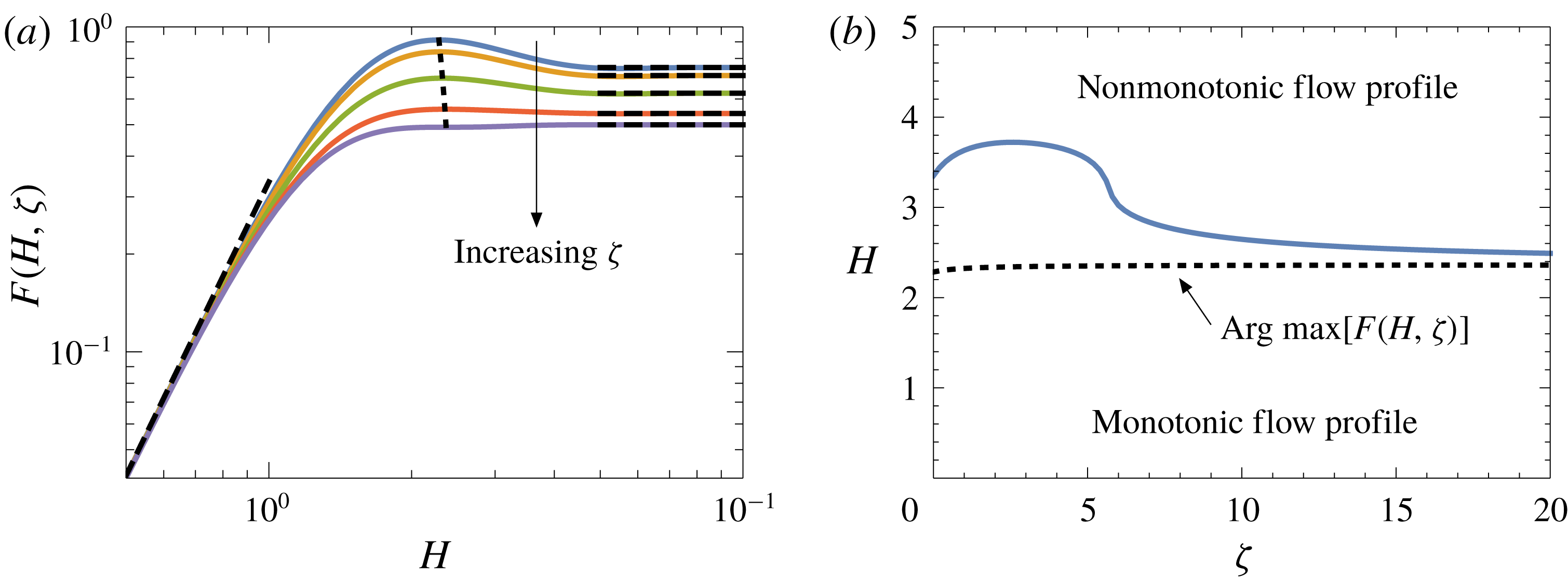
(a) The normalised flux function
 $F(H,\unicode[STIX]{x1D701})$
, given by (3.7), plotted versus
 $H$
with
 $\unicode[STIX]{x1D701}\in \{0,0.2,1,5,\infty \}$
; the dashed curves show the asymptotic limits (3.8) and the dotted curve shows the locus of the maximum value of
 $F$
, given implicitly by (3.10). (b) The
 $(\unicode[STIX]{x1D701},H)$
parameter space. The dotted black curve shows the maximising value
 $H$
of the function
 $F(H,\unicode[STIX]{x1D701})$
, defined implicitly as a function of
 $\unicode[STIX]{x1D701}$
by (3.9). The solid blue curve shows the boundary between parameter values where the flow profile is monotonic or non-monotonic.

For each fixed value of the parameter
 $\unicode[STIX]{x1D701}$
, the scaled flux
 $F(H,\unicode[STIX]{x1D701})$
is a non-monotonic function of the scaled thickness
 $H$
, as shown in figure 4(a). Note that the scaling factor
 $a\unicode[STIX]{x1D701}=\unicode[STIX]{x1D706}/r$
reflects the strength of the magnetic forces. As the film thickness tends to zero, viscous forces dominate magnetic effects, and the classical lubrication theory result is recovered, with
 $$\begin{eqnarray}\displaystyle F(H,\unicode[STIX]{x1D701})\sim \frac{H^{3}}{3}\quad \text{as }H\rightarrow 0. & & \displaystyle\end{eqnarray}$$
However, as the film thickness increases, the magnetic stress takes over, and the flux ultimately becomes independent of
 $H$
, with
 $$\begin{eqnarray}\displaystyle F(H,\unicode[STIX]{x1D701})\rightarrow \frac{1}{4}\left(2+\frac{1}{1+\unicode[STIX]{x1D701}}\right)\quad \text{as }H\rightarrow \infty . & & \displaystyle\end{eqnarray}$$
At intermediate values,
 $F(H,\unicode[STIX]{x1D701})$
is an oscillatory function of
 $H$
. The first extremal value of
 $H$
, corresponding to the global maximum in
 $F$
, is given as a function of
 $\unicode[STIX]{x1D701}$
by the implicit relation
 $$\begin{eqnarray}\displaystyle \unicode[STIX]{x1D701}=\frac{\cos 2H-2\sin H\sinh H-2\cos H\cosh H+1}{2\cos H\sinh H+2\sin H\cosh H}. & & \displaystyle\end{eqnarray}$$
As shown by the dotted black curve in figure 4(b), as
 $\unicode[STIX]{x1D701}$
ranges from
 $0$
to
 $\infty$
, the extremal value of
 $H$
increases monotonically from
 $H_{0}$
to
 $H_{\infty }$
, where
 $H_{0}\approx 2.284$
and
 $H_{\infty }\approx 2.365$
are the first positive zeros of the numerator and denominator, respectively, of the right-hand side of (3.9).
By substituting (3.9) into (3.7), we find that the maximum value of
 $F(H,\unicode[STIX]{x1D701})$
is given parametrically as a function of
 $\unicode[STIX]{x1D701}$
by (3.9) and
 $$\begin{eqnarray}\displaystyle \max F(H)=\frac{\sec H\sinh H+\tan H(\sec H\cosh H-2)}{4}, & & \displaystyle\end{eqnarray}$$
with
 $H\in (H_{0},H_{\infty })$
. The relation (3.10) is plotted as a dotted curve in figure 4(a). To the left of this dotted curve,
 $F$
is an increasing function of
 $H$
but, as
 $H$
increases past its extremal value,
 $F$
starts to decrease again and then to oscillate. We will argue below in § 3.2 that only the increasing branch of
 $F$
to the left of the dotted curve in figure 4(a) is relevant and, therefore, that no physical solutions exist in the region of
 $(\unicode[STIX]{x1D701},H)$
parameter space above the dotted curve in figure 4(b).
Figure 3(b) shows that the velocity profile becomes non-monotonic at larger values of
 $H$
; indeed the oscillations in the flow profile become increasingly dramatic as
 $H$
increases, and may even lead to flow reversal in the interior of the film. The solid blue curve in figure 4(b) shows the boundary between regions of the
 $(\unicode[STIX]{x1D701},H)$
parameter space where
 $u(y)$
is monotonic or non-monotonic. We note that non-monotonic solutions occur only for value of
 $(\unicode[STIX]{x1D701},H)$
above the black dotted curve in figure 4(b), showing the value of
 $H$
that maximises
 $F$
. We will thus contend in the next section that, although similar oscillatory flow profiles have been reported in the literature (Gao & Morley Reference Gao and Morley2002), they are unphysical and could never be observed in practice.
3.2 Steady states
We begin by letting all of the small parameters
 $\unicode[STIX]{x1D6FC}$
,
 $\unicode[STIX]{x1D6FD}$
and
 $\unicode[STIX]{x1D6E4}$
tend to zero so that
 $\unicode[STIX]{x1D711}(r,t)\equiv 1$
. We also consider the divertor to occupy the dimensionless interval
 $r\in [1,2]$
. Steady solutions
 $h_{0}(r)$
of (3.4) are then given by
 $$\begin{eqnarray}\displaystyle Q(h_{0}(r);r)=\frac{q}{r}, & & \displaystyle\end{eqnarray}$$
where the constant
 $q$
is set by specifying the inlet flux:
 $Q|_{r=1}=q$
.
Differentiation of (3.11) with respect to
 $r$
leads to
 $$\begin{eqnarray}\displaystyle \frac{\text{d}h_{0}}{\text{d}r}=-\left.\left(\frac{\unicode[STIX]{x2202}Q}{\unicode[STIX]{x2202}r}+\frac{q}{r^{2}}\right)\right/\frac{\unicode[STIX]{x2202}Q}{\unicode[STIX]{x2202}h}. & & \displaystyle\end{eqnarray}$$
By differentiating (3.7), we find that
 $$\begin{eqnarray}\displaystyle -r\frac{\text{d}}{\text{d}r}[\log (r^{1/3}h_{0}(r))]=-\frac{4}{3}+\frac{4F-\unicode[STIX]{x1D701}\unicode[STIX]{x2202}F/\unicode[STIX]{x2202}\unicode[STIX]{x1D701}}{H\unicode[STIX]{x2202}F/\unicode[STIX]{x2202}H}, & & \displaystyle\end{eqnarray}$$
where
 $F(H,\unicode[STIX]{x1D701})$
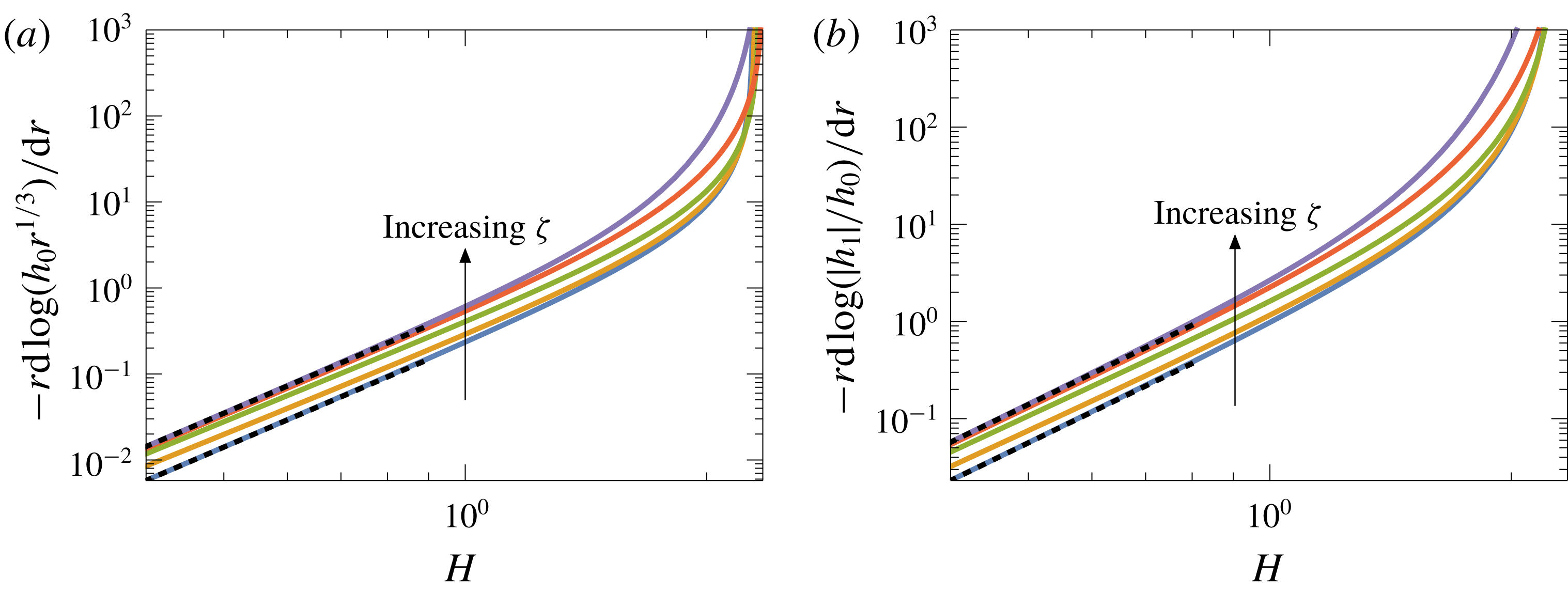
is the function defined in (3.7). This expression is uniformly positive (see figure 5
a), and it follows that
 $h_{0}(r)$
is a monotonic decreasing function which is bounded above by
 $h_{0}(1)/r^{1/3}$
. However, as the imposed flux
 $q$
increases, so too does the film thickness at the inlet, eventually approaching the maximum of
 $Q$
, where
 , so that the denominator of the (3.12) approaches zero and the free surface forms a gradient singularity.
(a) The normalised
 $r$
-derivative of the steady state solution
 $h_{0}(r)$
, defined by (3.13), plotted versus
 $H$
with
 $\unicode[STIX]{x1D701}\in \{0,0.2,1,5,\infty \}$
. The black dotted lines show the asymptotic behaviour as
 $H\rightarrow 0$
, namely
 $71H^{4}/315$
(
 $\unicode[STIX]{x1D701}=0$
),
 $176H^{4}/315$
(
 $\unicode[STIX]{x1D701}>0$
). (b) The right-hand side of (3.21) plotted versus
 $H$
with
 $\unicode[STIX]{x1D701}\in \{0,0.2,1,5,\infty \}$
. The black dotted lines show the asymptotic behaviour as
 $H\rightarrow 0$
, namely
 $284H^{4}/315$
(
 $\unicode[STIX]{x1D701}=0$
),
 $704H^{4}/315$
(
 $\unicode[STIX]{x1D701}>0$
).

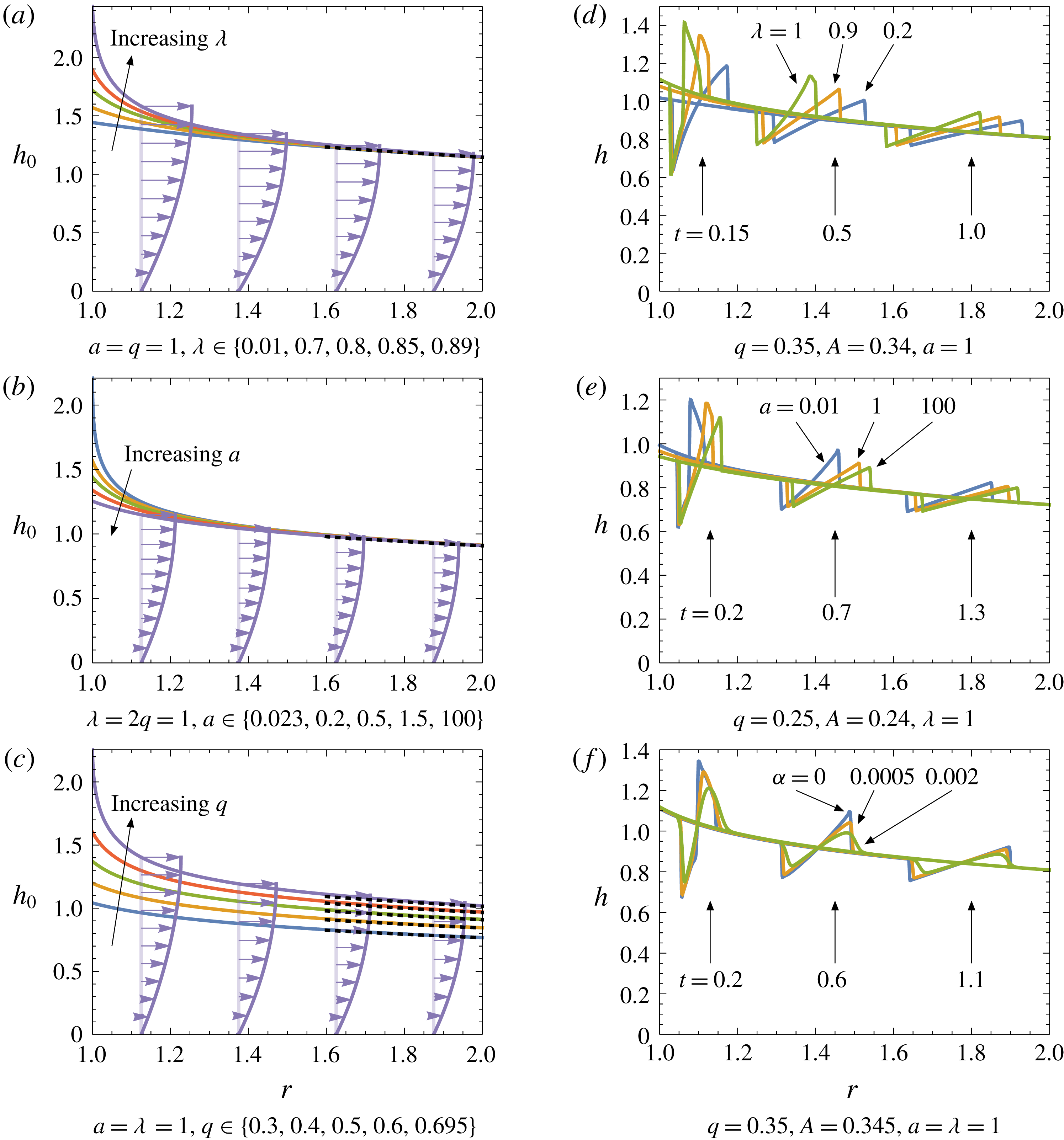
Solutions of (3.11) for
 $h_{0}(r)$
with various values of the parameters
 $\unicode[STIX]{x1D706}$
,
 $a$
and
 $q$
are plotted in figure 6(a–c). In figure 6(a) we observe that increasing the normalised field strength
 $\unicode[STIX]{x1D706}$
causes higher free surfaces due to increased magnetic drag on the flow. Figure 6(b) demonstrates that increasing the conductivity of the substrate (decreasing
 $a$
) likewise decreases the flow velocity and thus increases the film thickness. Finally, in figure 6(c) we show the effects of increasing the flux, which acts to increase the film thickness globally. Since both
 $H$
and
 $\unicode[STIX]{x1D701}$
tend to zero, the viscous dominated behaviour (3.8a
) applies in the limit as
 $r\rightarrow \infty$
, and thus (3.11) implies that
 $$\begin{eqnarray}\displaystyle h_{0}(r)\sim \left(\frac{3q}{r}\right)^{1/3}\quad \text{as }r\rightarrow \infty . & & \displaystyle\end{eqnarray}$$
This limit is plotted as the black dotted curves in figure 6(a–c). In each of figure 6(a,b) the value of the flux
 $q$
is held constant, as a consequence of which the free-surface profiles all converge as
 $r\rightarrow \infty$
.
(a–c) Steady free-surface solutions of (3.11) with the large-
 $r$
limit (3.14) overlaid as black dotted curves, and the corresponding velocity profiles. (d–f) Snapshots of numerical simulations for the film thickness
 $h(r,t)$
, satisfying equation (3.4), at the indicated times, with the time-dependent inlet flux given by (3.15).

Crucially, each of the solutions plotted in figure 6(a) to 6(c) exhibits a critical value of
 $\unicode[STIX]{x1D706}$
,
 $a$
, and
 $q$
, respectively, at which a singularity forms in the free surface, associated with
 $\unicode[STIX]{x2202}Q/\unicode[STIX]{x2202}h$
tending to zero at the inlet
 $r=1$
. Beyond each of these critical values, no steady free surface profile exists along the full extent of the divertor. The origin of the free-surface singularity may also be understood by considering the time-dependent problem (3.4). When
 $\unicode[STIX]{x1D711}\equiv 1$
, equation (3.4) is a first-order nonlinear hyperbolic partial differential equation (PDE), with characteristics satisfying
 . As the value of
 at
 $r=1$
changes sign, the characteristics cease to point into the domain, and it becomes impossible to specify the flux at the inlet.
Since, as shown in figure 4(a),
 $Q$
is an oscillatory function of
 $h$
, there may be further regions of parameter space in which
 becomes positive again, but we now argue that such branches cannot be physical. As shown above,
 $h_{0}(r)$
is a monotonic decreasing function, and it follows that, as
 $r$
increases, a singular point where
 tends to zero is necessarily encountered within a finite (and in practice very small) extent, so there still cannot exist steady solutions for an arbitrarily long divertor.
Therefore, when
 $\unicode[STIX]{x1D711}\equiv 1$
, smooth steady profiles only exist in the ‘subcritical’ region of parameter space below the dotted black curve in figure 4(b). This constraint places a strict bound on the value of
 $Q$
(or, equivalently,
 $h$
) imposed at the inlet. Importantly, figure 4(b) demonstrates that the non-monotonic velocity profiles seen, for example, in figure 3(b) occur for supercritical parameter values corresponding to unphysical steady state solutions, and we therefore do not expect to observe such exotic profiles in the wild.
3.3 Unsteady solutions
In this section we consider unsteady solutions of the governing equation (3.4), again neglecting the higher-order effects of transverse gravity and surface tension in the first instance, so that
 $\unicode[STIX]{x1D711}\equiv 1$
. We solve the resulting nonlinear hyperbolic equation numerically using the Kurganov–Tadmor scheme (Kurganov & Tadmor Reference Kurganov and Tadmor2000) with the parameter-free Superbee limiter (Roe Reference Roe1986). For the purposes of illustration, we initiate the simulation at the steady-state film profile,
 $h(r,0)=h_{0}(r)$
with specified flux
 $q$
, and subsequently perturb the inlet flux by one period of a sinusoid by applying the boundary condition
 $$\begin{eqnarray}\displaystyle Q=q+A\sin (60t)\unicode[STIX]{x1D6F1}(2\unicode[STIX]{x03C0}/60-t)\quad \text{at }r=1\text{ for }t>0, & & \displaystyle\end{eqnarray}$$
where
 $\unicode[STIX]{x1D6F1}$
is the Heaviside function. The values of
 $q$
and
 $A$
are chosen to ensure that the criticality bound described in § 3.2 is never exceeded, and the hyperbolic evolution problem thus remains well posed for all time.
In figure 6(d,e) we plot the computed free-surface profiles at various times and for various values of
 $q$
,
 $A$
,
 $\unicode[STIX]{x1D706}$
and
 $a$
. We observe that, despite the smooth profile of the inlet perturbation, the free surface develops a sawtooth appearance, due to wave steepening that results in the formation of shocks and rarefactions, typical of nonlinear wave propagation. We also observe that either a higher field strength (larger
 $\unicode[STIX]{x1D706}$
) or a more conducting substrate (smaller
 $a$
) slows the propagation of the disturbance (in particular the higher free-surface heights), but does not necessarily lead to the disturbance magnitude being damped. This is consistent with our observations for the steady case where these two effects both lead to a higher free surface due to increased drag.
Finally, in figure 6(f), we relax the assumption that
 $\unicode[STIX]{x1D711}\equiv 1$
to demonstrate how the sharp sawtooth is regularised by small contributions of the higher-order effects; here we reintroduce transverse gravity, by using small but non-zero values of the parameter
 $\unicode[STIX]{x1D6FC}$
, while still neglecting surface tension. When introducing higher-order derivatives, we must impose the correct number of associated boundary conditions for the problem to be well posed. In the simulations shown in figure 6(f), we impose the flux condition (3.15) at the inlet and a passive zero-derivative boundary condition
 at the outlet
 $r=2$
. The results show that more diffusion (larger
 $\unicode[STIX]{x1D6FC}$
) does not change the propagation speed but smooths the slope discontinuities and somewhat dampens the perturbation magnitude.
3.4 Linear stability analysis
The simulations plotted in figure 6(d–f) display no growth of the perturbations as they propagate downstream, suggesting that the steady-state free-surface profile is stable. We now investigate this behaviour analytically by looking at the linear stability of the system. Let us suppose that the inlet flux at
 $r=1$
is subject to small-amplitude time-harmonic fluctuations, so that
 $$\begin{eqnarray}\displaystyle Q=q+\unicode[STIX]{x1D6FF}\text{e}^{-\text{i}\unicode[STIX]{x1D714}t}\quad \text{at }r=1, & & \displaystyle\end{eqnarray}$$
where the frequency
 $\unicode[STIX]{x1D714}$
is specified and
 $0<\unicode[STIX]{x1D6FF}\ll 1$
. Since the coefficients of
 $h$
vary in space in the governing equation (3.4), we consider perturbations to the free-surface profile of the form
 $$\begin{eqnarray}\displaystyle h=h_{0}(r)+\unicode[STIX]{x1D6FF}h_{1}(r)\text{e}^{-\text{i}\unicode[STIX]{x1D714}t}, & & \displaystyle\end{eqnarray}$$
where
 $h_{0}(r)$
is the steady-state solution. Substituting (3.17) into (3.4) and neglecting terms of
 $O(\unicode[STIX]{x1D6FF}^{2})$
, we obtain the equation
 $$\begin{eqnarray}\displaystyle \frac{1}{h_{1}}\frac{\text{d}h_{1}}{\text{d}r}=-\left(\frac{\unicode[STIX]{x2202}Q}{\unicode[STIX]{x2202}h}\right)^{-1}\left[-\text{i}\unicode[STIX]{x1D714}+\frac{1}{r}\frac{\text{d}}{\text{d}r}\left(r\frac{\unicode[STIX]{x2202}Q}{\unicode[STIX]{x2202}h}\right)\right], & & \displaystyle\end{eqnarray}$$
subject to the boundary condition
 $$\begin{eqnarray}\displaystyle h_{1}=\left(\frac{\unicode[STIX]{x2202}Q}{\unicode[STIX]{x2202}h}\right)^{-1}\quad \text{at }r=1, & & \displaystyle\end{eqnarray}$$
where derivatives of
 $Q$
are evaluated at
 $(h_{0}(r);r)$
.
The solution of the problem (3.18) may be expressed in the form
 $$\begin{eqnarray}\displaystyle h_{1}(r)=\left(r\frac{\unicode[STIX]{x2202}Q}{\unicode[STIX]{x2202}h}(h_{0}(r);r)\right)^{-1}\exp \left(\text{i}\unicode[STIX]{x1D714}\int _{1}^{r}\left(\frac{\unicode[STIX]{x2202}Q}{\unicode[STIX]{x2202}h}(h_{0}(s);s)\right)^{-1}\,\text{d}s\right). & & \displaystyle\end{eqnarray}$$
The perturbation in (3.19) evidently comprises a spatially dependent amplitude function
 $$\begin{eqnarray}\displaystyle |h_{1}(r)|=\left(r\frac{\unicode[STIX]{x2202}Q}{\unicode[STIX]{x2202}h}(h_{0}(r);r)\right)^{-1}, & & \displaystyle\end{eqnarray}$$
multiplied by an exponential oscillatory term which captures all the
 $\unicode[STIX]{x1D714}$
-dependence and has modulus
 $1$
. To explore the behaviour of the perturbation amplitude (3.20), we compute
 $$\begin{eqnarray}\displaystyle -r\frac{\text{d}}{\text{d}r}\log (|h_{1}|/h_{0})=H\frac{\unicode[STIX]{x2202}}{\unicode[STIX]{x2202}H}\left(\frac{4F-\unicode[STIX]{x1D701}\unicode[STIX]{x2202}F/\unicode[STIX]{x2202}\unicode[STIX]{x1D701}}{H\unicode[STIX]{x2202}F/\unicode[STIX]{x2202}H}\right), & & \displaystyle\end{eqnarray}$$
where
 $F$
is again the expression given in (3.7). The expression on the right-hand side of (3.21) is a positive increasing function of
 $H$
, which tends to infinity as
 $H$
approaches the critical maximal value where
 (see figure 5
b). We deduce that, as
 $r$
increases, the perturbation amplitude
 $|h_{1}(r)|$
decreases monotonically relative to the leading-order film thickness
 $h_{0}(r)$
, and therefore respects the upper bounds
 $$\begin{eqnarray}\displaystyle |h_{1}(r)|\leqslant \frac{|h_{1}(1)|}{h_{0}(1)}h_{0}(r)\leqslant \frac{|h_{1}(1)|}{r^{1/3}}. & & \displaystyle\end{eqnarray}$$
The analysis of this section appears to show that there is no possibility of the steady base state suffering a linear instability. However, our governing thin-film (3.4) was derived by setting
 $Re^{\ast }=0$
and thus assuming that inertia effects are uniformly negligible. In the next section, we perform a more detailed stability analysis that relaxes this assumption.
4 High-frequency stability analysis
4.1 Synopsis
We start by outlining the derivations and analysis to follow, to guide the reader through the technical details. In § 4.2 we perform a multiple-scale perturbation analysis of the underlying (2.35) and (2.36) to produce a linearised system governing small perturbations that act over sufficiently small space and time scales for inertial effects to become important. We seek separable solutions in the form of harmonic waves propagating in the
 $r$
-direction, and thus ultimately obtain a generalised eigenvalue problem that, in principle, determines the linearised wave speed
 $c$
as a function of the wavenumber
 $k$
. This eigenvalue problem is normalised in § 4.3 to reduce the number of independent parameters in the problem. Our focus then is on studying how the normalised wave speed
 $\mathfrak{c}$
depends on the normalised wavenumber
 $\unicode[STIX]{x1D705}$
. In particular, we want to determine whether the imaginary part of
 $\mathfrak{c}$
is positive for any
 $\unicode[STIX]{x1D705}\in (0,\infty )$
, in which case the base state is linearly unstable. To this end, we analyse in detail the limiting behaviours as
 $\unicode[STIX]{x1D705}\rightarrow 0$
and as
 $\unicode[STIX]{x1D705}\rightarrow \infty$
in §§ 4.4 and 4.5, respectively.
In the small-
 $\unicode[STIX]{x1D705}$
limit, we find that there are two families of solution branches: § 4.4.1 concerns the bounded branch, on which
 $\mathfrak{c}$
tends to a constant, while § 4.4.2 concerns the divergent branches, on which
 $\mathfrak{c}$
tends to infinity as
 $\unicode[STIX]{x1D705}\rightarrow 0$
. Our analysis reveals the set of parameter values for which the steady base state is stable in the limit
 $\unicode[STIX]{x1D705}\rightarrow 0$
, corresponding to arbitrarily long waves, thus generalising the hydrodynamic stability analysis of Yih (Reference Yih1963). The corresponding large-
 $\unicode[STIX]{x1D705}$
analysis in § 4.5 establishes that, for all parameter values,
 $\text{Im}[\mathfrak{c}]$
is ultimately negative in the limit as
 $\unicode[STIX]{x1D705}\rightarrow \infty$
, and thus that the base state is stable to perturbations with arbitrarily small wavelength.
A numerical approach to determine
 $\mathfrak{c}$
for any value of
 $\unicode[STIX]{x1D705}$
is described in § 4.6. We find that the different solution branches identified in § 4.4 may intersect and switch places, and it is therefore necessary to track all relevant branches carefully as
 $\unicode[STIX]{x1D705}$
is varied. For certain parameter values, although the problem is predicted to be stable in the limits as
 $\unicode[STIX]{x1D705}\rightarrow 0$
and as
 $\unicode[STIX]{x1D705}\rightarrow \infty$
, the sign of
 $\text{Im}[\unicode[STIX]{x1D705}]$
may change at intermediate values of
 $\unicode[STIX]{x1D705}$
and thus render the problem unstable to finite-wavelength perturbations.
Finally, in § 4.7 we summarise the results of the stability analysis and explain their real-world relevance. In particular, we show how the critical Reynolds number, below which the steady base flow is stable, varies with the physical parameters in the problem.
4.2 Multiple-scale perturbation
Here we consider the stability of high-frequency disturbances on time and length scales that are small enough for inertia effects to become significant, despite the smallness of
 $Re^{\ast }$
. With the inertia terms reinstated, the thin-film problem (2.35) and (2.36) becomes
 $$\begin{eqnarray}\displaystyle & \displaystyle \frac{\unicode[STIX]{x2202}^{2}B^{i}}{\unicode[STIX]{x2202}y^{2}}+\frac{u}{r^{2}}=0, & \displaystyle\end{eqnarray}$$
 $$\begin{eqnarray}\displaystyle & \displaystyle \frac{1}{r}\frac{\unicode[STIX]{x2202}}{\unicode[STIX]{x2202}r}(ru)+\frac{\unicode[STIX]{x2202}v}{\unicode[STIX]{x2202}y}=0, & \displaystyle\end{eqnarray}$$
 $$\begin{eqnarray}\displaystyle & \displaystyle Re^{\ast }\left(\frac{\unicode[STIX]{x2202}u}{\unicode[STIX]{x2202}t}+u\frac{\unicode[STIX]{x2202}u}{\unicode[STIX]{x2202}r}+v\frac{\unicode[STIX]{x2202}u}{\unicode[STIX]{x2202}y}\right)-\frac{\unicode[STIX]{x2202}^{2}u}{\unicode[STIX]{x2202}y^{2}}+4\unicode[STIX]{x1D706}^{4}\frac{B^{i}}{r^{2}}=\unicode[STIX]{x1D711}(r,t), & \displaystyle\end{eqnarray}$$
 $$\begin{eqnarray}\displaystyle & \displaystyle u=v=\frac{\unicode[STIX]{x2202}B^{i}}{\unicode[STIX]{x2202}y}-aB^{i}=0\quad \text{at }y=0, & \displaystyle\end{eqnarray}$$
 $$\begin{eqnarray}\displaystyle & \displaystyle \frac{\unicode[STIX]{x2202}u}{\unicode[STIX]{x2202}y}=v-\frac{\unicode[STIX]{x2202}h}{\unicode[STIX]{x2202}t}-u\frac{\unicode[STIX]{x2202}h}{\unicode[STIX]{x2202}r}=B^{i}=0\quad \text{at }y=h(r,t). & \displaystyle\end{eqnarray}$$
Let
 $u_{0}(r,y)$
,
 $v_{0}(r,y)$
,
 $B_{0}(r,y)$
and
 $h_{0}(r)$
refer to steady-state solutions of the leading-order (inertia-free) model, as constructed in § 3.2. We now perform a multiple-scale perturbation about this base state, setting
 $$\begin{eqnarray}\displaystyle & \displaystyle u\sim u_{0}(r,y)+Re^{\ast }u_{1}(\hat{r},r,y,\hat{t})+\cdots \,, & \displaystyle\end{eqnarray}$$
 $$\begin{eqnarray}\displaystyle & \displaystyle B^{i}\sim B_{0}(r,y)+Re^{\ast }B_{1}(\hat{r},r,y,\hat{t})+\cdots \,, & \displaystyle\end{eqnarray}$$
 $$\begin{eqnarray}\displaystyle & \displaystyle v\sim v_{0}(r,y)+v_{1}(\hat{r},r,y,\hat{t})+\cdots \,, & \displaystyle\end{eqnarray}$$
 $$\begin{eqnarray}\displaystyle & \displaystyle h\sim h_{0}(r)+Re^{\ast }h_{1}(\hat{r},r,\hat{t})+\cdots \,, & \displaystyle\end{eqnarray}$$
 $$\begin{eqnarray}\displaystyle \hat{r}=\frac{r}{Re^{\ast }},\quad \hat{t}=\frac{t}{Re^{\ast }} & & \displaystyle\end{eqnarray}$$
are fast length and time variables. We substitute (4.3) into (4.1) and (4.2) and then take the asymptotic limit
 $Re^{\ast }\rightarrow 0$
. To proceed, we have to decide how to decompose the pressure gradient term
 $\unicode[STIX]{x1D711}$
in powers of
 $Re^{\ast }$
. Bearing in mind the relative typical sizes of the parameters
 $\unicode[STIX]{x1D6FC}$
,
 $\unicode[STIX]{x1D6FD}$
,
 $\unicode[STIX]{x1D6E4}$
and
 $Re^{\ast }$
given in (2.34), and aiming to include transverse gravity and surface tension at first order, we define
 $\unicode[STIX]{x1D711}\sim \unicode[STIX]{x1D711}_{0}(r)+Re^{\ast }\unicode[STIX]{x1D711}_{1}(\hat{r},r,y,\hat{t})+\cdots \,$
, with
 $$\begin{eqnarray}\displaystyle \unicode[STIX]{x1D711}_{0}=1-\frac{2\unicode[STIX]{x1D6FD}}{r^{3}},\quad \unicode[STIX]{x1D711}_{1}=-\hat{\unicode[STIX]{x1D6FC}}\left(\frac{\text{d}h_{0}}{\text{d}r}+\frac{\unicode[STIX]{x2202}h_{1}}{\unicode[STIX]{x2202}\hat{r}}\right)+\hat{\unicode[STIX]{x1D6E4}}\frac{\unicode[STIX]{x2202}^{3}h_{1}}{\unicode[STIX]{x2202}\hat{r}^{3}}, & & \displaystyle\end{eqnarray}$$
where
 $$\begin{eqnarray}\displaystyle \hat{\unicode[STIX]{x1D6FC}}=\frac{\unicode[STIX]{x1D6FC}}{Re^{\ast }},\quad \hat{\unicode[STIX]{x1D6E4}}=\frac{\unicode[STIX]{x1D6E4}}{{Re^{\ast }}^{3}}. & & \displaystyle\end{eqnarray}$$
The leading-order governing equations and boundary conditions are satisfied identically, by construction. At
 $O(Re^{\ast })$
, we obtain the governing equations
 $$\begin{eqnarray}\displaystyle \frac{\unicode[STIX]{x2202}^{2}B_{1}}{\unicode[STIX]{x2202}y^{2}}+\frac{u_{1}}{r^{2}}=\frac{\unicode[STIX]{x2202}u_{1}}{\unicode[STIX]{x2202}\hat{r}}+\frac{\unicode[STIX]{x2202}v_{1}}{\unicode[STIX]{x2202}y}=0, & & \displaystyle\end{eqnarray}$$
 $$\begin{eqnarray}\displaystyle & & \displaystyle \frac{\unicode[STIX]{x2202}u_{1}}{\unicode[STIX]{x2202}\hat{t}}+u_{0}\frac{\unicode[STIX]{x2202}u_{1}}{\unicode[STIX]{x2202}\hat{r}}+\frac{\unicode[STIX]{x2202}u_{0}}{\unicode[STIX]{x2202}y}v_{1}-\frac{\unicode[STIX]{x2202}^{2}u_{1}}{\unicode[STIX]{x2202}y^{2}}+4\unicode[STIX]{x1D706}^{4}\frac{B_{1}}{r^{2}}+\hat{\unicode[STIX]{x1D6FC}}\frac{\unicode[STIX]{x2202}h_{1}}{\unicode[STIX]{x2202}\hat{r}}-\hat{\unicode[STIX]{x1D6E4}}\frac{\unicode[STIX]{x2202}^{3}h_{1}}{\unicode[STIX]{x2202}\hat{r}^{3}}\nonumber\\ \displaystyle & & \displaystyle \quad =-\hat{\unicode[STIX]{x1D6FC}}\frac{\text{d}h_{0}}{\text{d}r}-u_{0}\frac{\unicode[STIX]{x2202}u_{0}}{\unicode[STIX]{x2202}r}-v_{0}\frac{\unicode[STIX]{x2202}u_{0}}{\unicode[STIX]{x2202}y},\end{eqnarray}$$
 $$\begin{eqnarray}\displaystyle & \displaystyle u_{1}=v_{1}=\frac{\unicode[STIX]{x2202}B_{1}}{\unicode[STIX]{x2202}y}-aB_{1}=0\quad \text{at }y=0, & \displaystyle\end{eqnarray}$$
 $$\begin{eqnarray}\displaystyle & \displaystyle \frac{\unicode[STIX]{x2202}u_{1}}{\unicode[STIX]{x2202}y}+\frac{\unicode[STIX]{x2202}^{2}u_{0}}{\unicode[STIX]{x2202}y^{2}}h_{1}=B_{1}+\frac{\unicode[STIX]{x2202}B_{0}}{\unicode[STIX]{x2202}y}h_{1}=v_{1}-\frac{\unicode[STIX]{x2202}h_{1}}{\unicode[STIX]{x2202}\hat{t}}-u_{0}\frac{\unicode[STIX]{x2202}h_{1}}{\unicode[STIX]{x2202}\hat{r}}=0\quad \text{at }y=h_{0}(r). & \displaystyle\end{eqnarray}$$
The inhomogeneous right-hand side of (4.7b
) is a function only of the slow variables
 $(r,y)$
, and may be eliminated by considering a particular integral
 $\{u_{1p}(r,y),B_{1p}(r,y)\}$
satisfying the boundary-value problem
 $$\begin{eqnarray}\displaystyle & \displaystyle \frac{\unicode[STIX]{x2202}^{2}B_{1p}}{\unicode[STIX]{x2202}y^{2}}+\frac{u_{1p}}{r^{2}}=0, & \displaystyle\end{eqnarray}$$
 $$\begin{eqnarray}\displaystyle & \displaystyle -\frac{\unicode[STIX]{x2202}^{2}u_{1p}}{\unicode[STIX]{x2202}y^{2}}+4\unicode[STIX]{x1D706}^{4}\frac{B_{1p}}{r^{2}}=-\hat{\unicode[STIX]{x1D6FC}}\frac{\text{d}h_{0}}{\text{d}r}-u_{0}\frac{\unicode[STIX]{x2202}u_{0}}{\unicode[STIX]{x2202}r}-v_{0}\frac{\unicode[STIX]{x2202}u_{0}}{\unicode[STIX]{x2202}y}, & \displaystyle\end{eqnarray}$$
 $$\begin{eqnarray}\displaystyle & \displaystyle u_{1p}(r,0)=\frac{\unicode[STIX]{x2202}B_{1p}}{\unicode[STIX]{x2202}y}(r,0)-aB_{1p}(r,0)=\frac{\unicode[STIX]{x2202}u_{1p}}{\unicode[STIX]{x2202}y}(r,h_{0}(r))=B_{1p}(r,h_{0}(r))=0. & \displaystyle\end{eqnarray}$$
 $r$
, and in principle explicit, although unwieldy, solutions may be found for
 $u_{1p}$
and
 $B_{1p}$
. For our purposes, it suffices to note that, since that the leading-order problem (3.3) is well posed, so too is (4.9), and by subtracting off the resulting particular integral, we can henceforth focus on the homogeneous version of (4.7b
) where the right-hand side is replaced by zero.
The resulting problem is linear and autonomous in
 $\hat{t}$
and
 $\hat{r}$
, and depends only parametrically on
 $r$
. We therefore suppress the dependence on
 $r$
, for the moment, and seek separable harmonic solutions of wavenumber
 $k$
and wave speed
 $c$
, that is,
 $$\begin{eqnarray}\displaystyle u_{1}=u_{1p}+\hat{u} (y)\text{e}^{\text{i}k(\hat{r}-c\hat{t})},\quad v_{1}=\hat{v}(y)\text{e}^{\text{i}k(\hat{r}-c\hat{t})}, & & \displaystyle\end{eqnarray}$$
 $$\begin{eqnarray}\displaystyle B_{1}=B_{1p}+\hat{B}(y)\text{e}^{\text{i}k(\hat{r}-c\hat{t})},\quad h_{1}={\hat{h}}\text{e}^{\text{i}k(\hat{r}-c\hat{t})}, & & \displaystyle\end{eqnarray}$$
which results in the ODE problem
 $$\begin{eqnarray}\displaystyle & \displaystyle \frac{\text{d}^{2}\hat{B}}{\text{d}y^{2}}+\frac{\hat{u} }{r^{2}}=\frac{\text{d}\hat{v}}{\text{d}y}+\text{i}k\hat{u} =0, & \displaystyle\end{eqnarray}$$
 $$\begin{eqnarray}\displaystyle & \displaystyle \text{i}k(u_{0}-c)\hat{u} +\frac{\text{d}u_{0}}{\text{d}y}\hat{v}-\frac{\text{d}^{2}\hat{u} }{\text{d}y^{2}}+\frac{4\unicode[STIX]{x1D706}^{4}}{r^{2}}\hat{B}+\text{i}k(\hat{\unicode[STIX]{x1D6FC}}+\hat{\unicode[STIX]{x1D6E4}}k^{2}){\hat{h}}=0, & \displaystyle\end{eqnarray}$$
 $$\begin{eqnarray}\displaystyle & \displaystyle \hat{u} =\hat{v}=\frac{\text{d}\hat{B}}{\text{d}y}-a\hat{B}=0\quad \text{at }y=0, & \displaystyle\end{eqnarray}$$
 $$\begin{eqnarray}\displaystyle & \displaystyle \frac{\text{d}\hat{u} }{\text{d}y}-\unicode[STIX]{x1D711}_{0}{\hat{h}}=\hat{B}+\frac{\text{d}B_{0}}{\text{d}y}{\hat{h}}=\hat{v}-\text{i}k(u_{0}-c){\hat{h}}=0\quad \text{at }y=h_{0}. & \displaystyle\end{eqnarray}$$
 $\hat{B}$
to the magnetic field.
We can eliminate
 $\hat{u}$
and
 $\hat{B}$
from (4.11) and thus obtain a single ODE for
 $\hat{v}(y)$
, namely
 $$\begin{eqnarray}\displaystyle \frac{\text{d}^{4}\hat{v}}{\text{d}y^{4}}+\text{i}k(c-u_{0})\frac{\text{d}^{2}\hat{v}}{\text{d}y^{2}}+\left(\frac{4\unicode[STIX]{x1D706}^{4}}{r^{4}}+\text{i}k\frac{\text{d}^{2}u_{0}}{\text{d}y^{2}}\right)\hat{v}+\frac{4\text{i}ka\unicode[STIX]{x1D706}^{4}}{r^{2}}\hat{B}(0)=0, & & \displaystyle\end{eqnarray}$$
which is subject to
 $$\begin{eqnarray}\displaystyle \hat{v}=\frac{\text{d}\hat{v}}{\text{d}y}=\frac{\text{d}^{3}\hat{v}}{\text{d}y^{3}}-k^{2}(\hat{\unicode[STIX]{x1D6FC}}+\hat{\unicode[STIX]{x1D6E4}}k^{2}){\hat{h}}+\frac{4\text{i}k\unicode[STIX]{x1D706}^{4}\hat{B}(0)}{r^{2}}=0\quad \text{at }y=0, & & \displaystyle\end{eqnarray}$$
 $$\begin{eqnarray}\displaystyle & & \displaystyle \hat{v}-\text{i}k(u_{0}-c){\hat{h}}=\frac{\text{d}^{2}\hat{v}}{\text{d}y^{2}}+\text{i}k\unicode[STIX]{x1D711}_{0}{\hat{h}}\nonumber\\ \displaystyle & & \displaystyle \quad =\frac{\text{d}^{3}\hat{v}}{\text{d}y^{3}}-\text{i}k(u_{0}-c)\frac{\text{d}\hat{v}}{\text{d}y}-\left(k^{2}(\hat{\unicode[STIX]{x1D6FC}}+\hat{\unicode[STIX]{x1D6E4}}k^{2})+\frac{4\text{i}k\unicode[STIX]{x1D706}^{4}}{r^{2}}\frac{\text{d}B_{0}}{\text{d}y}\right){\hat{h}}=0\quad \text{at }y=h_{0}.\qquad \quad\end{eqnarray}$$
4.3 Normalised problem
We normalise the leading-order solutions
 $u_{0}$
and
 $B_{0}$
using (3.1) and (3.2) as in § 3.1, and similarly scale the first-order problem as follows:
 $$\begin{eqnarray}\displaystyle \hat{v}(y)=-\frac{4\text{i}ka\unicode[STIX]{x1D706}^{4}h_{0}^{4}\hat{B}(0)}{r^{2}}{\mathcal{V}}(Y),\quad k=\frac{\unicode[STIX]{x1D706}^{2}}{\unicode[STIX]{x1D711}_{0}r^{2}h_{0}^{2}}\unicode[STIX]{x1D705},\quad \hat{\unicode[STIX]{x1D6FC}}=\unicode[STIX]{x1D711}_{0}^{2}h_{0}^{3}\tilde{\unicode[STIX]{x1D6FC}}, & & \displaystyle\end{eqnarray}$$
 $$\begin{eqnarray}\displaystyle {\hat{h}}=\frac{4a\unicode[STIX]{x1D706}^{2}H^{4}\hat{B}(0)}{\unicode[STIX]{x1D711}_{0}}{\mathcal{H}},\quad c=\frac{\unicode[STIX]{x1D711}_{0}}{a^{2}\unicode[STIX]{x1D701}^{2}}\mathfrak{c},\quad \hat{\unicode[STIX]{x1D6E4}}=\unicode[STIX]{x1D711}_{0}^{4}h_{0}^{11}\tilde{\unicode[STIX]{x1D6E4}}. & & \displaystyle\end{eqnarray}$$
We thus obtain the normalised equation
 $$\begin{eqnarray}\displaystyle \frac{\text{d}^{4}{\mathcal{V}}}{\text{d}Y^{4}}+\text{i}\unicode[STIX]{x1D705}(\mathfrak{c}-{\mathcal{U}})\frac{\text{d}^{2}{\mathcal{V}}}{\text{d}Y^{2}}+\left(4H^{4}+\text{i}\unicode[STIX]{x1D705}\frac{\text{d}^{2}{\mathcal{U}}}{\text{d}Y^{2}}\right){\mathcal{V}}=1, & & \displaystyle\end{eqnarray}$$
which is analogous to equation (4.2) in Stuart (Reference Stuart1954), albeit with a different form of the base flow
 ${\mathcal{U}}(Y)$
and also with different boundary conditions, namely
 $$\begin{eqnarray}\displaystyle & \displaystyle {\mathcal{V}}(0)=\frac{\text{d}{\mathcal{V}}}{\text{d}Y}(0)=\frac{\text{d}^{2}{\mathcal{V}}}{\text{d}Y^{2}}(1)-\frac{H^{2}}{\mathfrak{c}-{\mathcal{U}}(1)}{\mathcal{V}}(1)=0, & \displaystyle\end{eqnarray}$$
 $$\begin{eqnarray}\displaystyle & \displaystyle \frac{\text{d}^{3}{\mathcal{V}}}{\text{d}Y^{3}}(0)-\frac{\text{i}H^{4}\unicode[STIX]{x1D705}(\tilde{\unicode[STIX]{x1D6FC}}+H^{4}\tilde{\unicode[STIX]{x1D6E4}}\unicode[STIX]{x1D705}^{2})}{\mathfrak{c}-{\mathcal{U}}(1)}{\mathcal{V}}(1)=\frac{\unicode[STIX]{x1D701}}{H}. & \displaystyle\end{eqnarray}$$
In principle, the four boundary conditions (4.17) are sufficient to solve the ODE (4.16) for
 ${\mathcal{V}}(Y)$
, with the solution depending parametrically on the normalised wavenumber
 $\unicode[STIX]{x1D705}$
and wave speed
 $\mathfrak{c}$
, as well as on the parameters
 $H$
,
 $\unicode[STIX]{x1D701}$
,
 $\tilde{\unicode[STIX]{x1D6FC}}$
and
 $\tilde{\unicode[STIX]{x1D6E4}}$
. The remaining boundary condition
 $$\begin{eqnarray}\displaystyle \frac{\text{d}^{3}{\mathcal{V}}}{\text{d}Y^{3}}(1)+\text{i}\unicode[STIX]{x1D705}(\mathfrak{c}-{\mathcal{U}}(1))\frac{\text{d}{\mathcal{V}}}{\text{d}Y}(1)=\left(\text{i}H^{2}\unicode[STIX]{x1D705}(\tilde{\unicode[STIX]{x1D6FC}}+H^{4}\tilde{\unicode[STIX]{x1D6E4}}\unicode[STIX]{x1D705}^{2})-4\frac{\text{d}{\mathcal{B}}}{\text{d}Y}(1)\right)\frac{\text{d}^{2}{\mathcal{V}}}{\text{d}Y^{2}}(1) & & \displaystyle\end{eqnarray}$$
thus effectively provides an algebraic dispersion relation between
 $\mathfrak{c}$
and
 $\unicode[STIX]{x1D705}$
. The temporal stability of the base state then depends on the imaginary part of
 $\mathfrak{c}$
: if
 $\text{Im}[\unicode[STIX]{x1D705}\mathfrak{c}]$
is positive for any real value of
 $\unicode[STIX]{x1D705}$
, then the base state is linearly unstable; otherwise it is linearly stable. Since the problem (4.16)–(4.18) is invariant under the transformation
 $\{V,\unicode[STIX]{x1D705},c\}\mapsto \{\overline{V},-\unicode[STIX]{x1D705},\overline{c}\}$
(where the bar denotes complex conjugation), in practice we can restrict our attention to positive values of
 $\unicode[STIX]{x1D705}$
.
For any given values of the parameters
 $H$
,
 $\unicode[STIX]{x1D701}$
,
 $\tilde{\unicode[STIX]{x1D6FC}}$
,
 $\tilde{\unicode[STIX]{x1D6E4}}$
and the normalised wavenumber
 $\unicode[STIX]{x1D705}$
, the generalised eigenvalue problem (4.16)–(4.18) gives an infinite set of possible values for the wave speed
 $\mathfrak{c}$
, and we are interested in the one with the largest imaginary part. Numerical solution of the problem is discussed below in § 4.6, but first, to guide and validate the numerics, we examine the asymptotic limits as the wavenumber tends to zero or to infinity.
4.4 Small wavenumber limit
4.4.1 Bounded branch
We follow the approach of Yih (Reference Yih1963) to analyse the dispersion relation in the limit as
 $\unicode[STIX]{x1D705}\rightarrow 0$
. We find that limiting solutions of (4.16)–(4.18) fall into two possible classes: one in which
 $\mathfrak{c}$
is bounded and one in which
 $\mathfrak{c}$
scales with
 $1/\unicode[STIX]{x1D705}$
as
 $\unicode[STIX]{x1D705}\rightarrow 0$
. We begin by analysing the former case. Since the first-order coefficients of
 $\unicode[STIX]{x1D705}$
in (4.16)–(4.18) are pure imaginary, we seek solutions for
 ${\mathcal{V}}$
and
 $\mathfrak{c}$
as asymptotic expansions of the form
 $$\begin{eqnarray}\displaystyle {\mathcal{V}}(Y)\sim {\mathcal{V}}_{0}(Y)+\text{i}\unicode[STIX]{x1D705}{\mathcal{V}}_{1}(Y)+\cdots \,,\quad \mathfrak{c}\sim \mathfrak{c}_{0}+\text{i}\unicode[STIX]{x1D705}\mathfrak{c}_{1}+\cdots \,, & & \displaystyle\end{eqnarray}$$
where
 $\mathfrak{c}_{0}$
and
 $\mathfrak{c}_{1}$
are real. The steady base state is then stable or unstable, in the limit
 $\unicode[STIX]{x1D705}\rightarrow 0$
, depending on whether
 $\mathfrak{c}_{1}$
is negative or positive, respectively.
At leading order, we obtain the problem
 $$\begin{eqnarray}\displaystyle \frac{\text{d}^{4}{\mathcal{V}}_{0}}{\text{d}Y^{4}}+4H^{4}{\mathcal{V}}_{0}=1, & & \displaystyle\end{eqnarray}$$
subject to
 $$\begin{eqnarray}\displaystyle {\mathcal{V}}_{0}(0)=\frac{\text{d}{\mathcal{V}}_{0}}{\text{d}Y}(0)=\frac{\text{d}^{3}{\mathcal{V}}_{0}}{\text{d}Y^{3}}(0)-\frac{\unicode[STIX]{x1D701}}{H}=\frac{\text{d}^{3}{\mathcal{V}}_{0}}{\text{d}Y^{3}}(1)+4\frac{\text{d}{\mathcal{B}}}{\text{d}Y}(1)\frac{\text{d}^{2}{\mathcal{V}}_{0}}{\text{d}Y^{2}}(1)=0, & & \displaystyle\end{eqnarray}$$
and the leading-order wave speed is then found from
 $$\begin{eqnarray}\displaystyle \mathfrak{c}_{0}={\mathcal{U}}(1)+H^{2}{\mathcal{V}}_{0}(1)\!\left/\frac{\text{d}^{2}{\mathcal{V}}_{0}}{\text{d}Y^{2}}(1).\right. & & \displaystyle\end{eqnarray}$$
The solution of the boundary-value problem (4.20) and (4.21) may be written in the form
 $$\begin{eqnarray}\displaystyle {\mathcal{V}}_{0}(Y)=-\frac{\unicode[STIX]{x1D701}}{\displaystyle H^{4}\frac{\unicode[STIX]{x2202}}{\unicode[STIX]{x2202}H}\left[\frac{1}{H^{2}}\frac{\unicode[STIX]{x2202}^{3}\unicode[STIX]{x1D6F9}}{\unicode[STIX]{x2202}Y^{3}}(0;H)\right]}\left[\unicode[STIX]{x1D6F9}(Y;H)+H\frac{\unicode[STIX]{x2202}\unicode[STIX]{x1D6F9}}{\unicode[STIX]{x2202}H}(Y;H)-Y\frac{\unicode[STIX]{x2202}\unicode[STIX]{x1D6F9}}{\unicode[STIX]{x2202}Y}(Y;H)\right],\qquad & & \displaystyle\end{eqnarray}$$
where
 $\unicode[STIX]{x1D6F9}$
is the leading-order streamfunction, defined by
 $$\begin{eqnarray}\displaystyle \unicode[STIX]{x1D6F9}(Y;H)=\int _{0}^{Y}{\mathcal{U}}(\bar{Y})\,\text{d}\bar{Y}. & & \displaystyle\end{eqnarray}$$
By substituting (4.23) into (4.22), we find that the leading-order wave speed is given by
 $$\begin{eqnarray}\displaystyle \mathfrak{c}_{0}=\frac{\unicode[STIX]{x2202}F}{\unicode[STIX]{x2202}H}, & & \displaystyle\end{eqnarray}$$
where
 $F(H,\unicode[STIX]{x1D701})=H\unicode[STIX]{x1D6F9}(1;H)$
is equivalent to the normalised flux defined in (3.7). Thus the leading-order wave speed is just the characteristic wave speed of the underlying hyperbolic equation (4.22), a result that is also consistent with the simple linearised solution (3.19). The resulting behaviour of
 $\mathfrak{c}_{0}$
as a function of
 $H$
for varying
 $\unicode[STIX]{x1D701}$
is plotted in figure 7(a). Notably, the wave speed is positive for physically relevant values of
 $H$
, but tends to zero as
 $H$
approaches the critical value where
 .
(a) The leading-order wave speed
 $\mathfrak{c}_{0}$
; (b) the first-order wave speed
 $\mathfrak{c}_{1,0}$
evaluated at
 $\tilde{\unicode[STIX]{x1D6FC}}=0$
; (c) the coefficient
 $\mathfrak{c}_{1,\unicode[STIX]{x1D6FC}}$
in the first-order wave speed
 $\mathfrak{c}_{1}$
; (d) the critical value of
 $\tilde{\unicode[STIX]{x1D6FC}}$
for stability of long waves. All are plotted versus
 $H$
for
 $\unicode[STIX]{x1D701}\in \{0,0.2,1,5,\infty \}$
, with a grey dashed curve bounding the range of parameters where physical steady solutions exist. In (b), the black circle indicates the
 $\unicode[STIX]{x1D701}\rightarrow \infty$
curve crossing the horizontal axis at the critical value of
 $H$
. In (d), the black dotted curve shows the asymptotic behaviour
 $\tilde{\unicode[STIX]{x1D6FC}}_{c0}\rightarrow 2/5$
as
 $H\rightarrow 0$
.

The first-order problem reads
 $$\begin{eqnarray}\displaystyle \frac{\text{d}^{4}{\mathcal{V}}_{1}}{\text{d}Y^{4}}+4H^{4}{\mathcal{V}}_{1}=-\left(\mathfrak{c}_{0}-{\mathcal{U}}\right)\frac{\text{d}^{2}{\mathcal{V}}_{0}}{\text{d}Y^{2}}-{\mathcal{V}}_{0}\frac{\text{d}^{2}{\mathcal{U}}}{\text{d}Y^{2}}, & & \displaystyle\end{eqnarray}$$
subject to
 $$\begin{eqnarray}\displaystyle & \displaystyle {\mathcal{V}}_{1}(0)=\frac{\text{d}{\mathcal{V}}_{1}}{\text{d}Y}(0)=\frac{\text{d}^{3}{\mathcal{V}}_{1}}{\text{d}Y^{3}}(0)-\frac{H^{4}\tilde{\unicode[STIX]{x1D6FC}}{\mathcal{V}}_{0}(1)}{\mathfrak{c}_{0}-{\mathcal{U}}(1)}=0, & \displaystyle\end{eqnarray}$$
 $$\begin{eqnarray}\displaystyle & \displaystyle \frac{\text{d}^{3}{\mathcal{V}}_{1}}{\text{d}Y^{3}}(1)+4\frac{\text{d}{\mathcal{B}}}{\text{d}Y}(1)\frac{\text{d}^{2}{\mathcal{V}}_{1}}{\text{d}Y^{2}}(1)=H^{2}\tilde{\unicode[STIX]{x1D6FC}}\frac{\text{d}^{2}{\mathcal{V}}_{0}}{\text{d}Y^{2}}(1)-(\mathfrak{c}_{0}-{\mathcal{U}}(1))\frac{\text{d}{\mathcal{V}}_{0}}{\text{d}Y}(1), & \displaystyle\end{eqnarray}$$
 $$\begin{eqnarray}\displaystyle \mathfrak{c}_{1}=\left(H^{2}{\mathcal{V}}_{1}(1)-(\mathfrak{c}_{0}-{\mathcal{U}}(1))\frac{\text{d}^{2}{\mathcal{V}}_{1}}{\text{d}Y^{2}}(1)\right)\!\left/\frac{\text{d}^{2}{\mathcal{V}}_{0}}{\text{d}Y^{2}}(1).\right. & & \displaystyle\end{eqnarray}$$
It may be shown that the solutions for
 ${\mathcal{V}}_{1}$
and
 $\mathfrak{c}_{1}$
can only vary affinely with the stabilising gravitational parameter
 $\tilde{\unicode[STIX]{x1D6FC}}$
, i.e. we can write
 $$\begin{eqnarray}\displaystyle {\mathcal{V}}_{1}(Y)\equiv {\mathcal{V}}_{1,0}(Y)+\tilde{\unicode[STIX]{x1D6FC}}{\mathcal{V}}_{1,\unicode[STIX]{x1D6FC}}(Y),\quad \mathfrak{c}_{1}\equiv \mathfrak{c}_{1,0}+\tilde{\unicode[STIX]{x1D6FC}}\mathfrak{c}_{1,\unicode[STIX]{x1D6FC}}, & & \displaystyle\end{eqnarray}$$
and the coefficients
 $\mathfrak{c}_{1,0}$
and
 $\mathfrak{c}_{1,\unicode[STIX]{x1D6FC}}$
may thus be solved for independently. The terms proportional to
 $\tilde{\unicode[STIX]{x1D6FC}}$
are relatively straightforward to evaluate, in the forms
 $$\begin{eqnarray}\displaystyle & \displaystyle {\mathcal{V}}_{1,\unicode[STIX]{x1D6FC}}(Y)=\frac{1}{4H^{2}\unicode[STIX]{x2202}{\mathcal{B}}(0)/\unicode[STIX]{x2202}H}[4H^{3}{\mathcal{B}}(0){\mathcal{V}}_{0}(Y)-\unicode[STIX]{x1D701}\unicode[STIX]{x1D6F9}(Y)], & \displaystyle\end{eqnarray}$$
 $$\begin{eqnarray}\displaystyle & \displaystyle \mathfrak{c}_{1,\unicode[STIX]{x1D6FC}}=-HF(H,\unicode[STIX]{x1D701}), & \displaystyle\end{eqnarray}$$
 $F$
is again the function defined by (3.7). Explicit solutions can also be found for
 ${\mathcal{V}}_{1,0}$
and
 $\mathfrak{c}_{1,0}$
, but they are too long winded to reproduce here. The solutions for
 $\mathfrak{c}_{1,0}$
and
 $\mathfrak{c}_{1,\unicode[STIX]{x1D6FC}}$
are plotted versus
 $H$
for various values of
 $\unicode[STIX]{x1D701}$
in figure 7(b,c).
The coefficient
 $\mathfrak{c}_{1,0}$
may be positive or negative for physically relevant values of
 $\unicode[STIX]{x1D701}$
and
 $H$
. We note for future reference that, in the limit
 $\unicode[STIX]{x1D701}\rightarrow \infty$
, one can express
 $\mathfrak{c}_{1,0}$
in the form
 $$\begin{eqnarray}\displaystyle \mathfrak{c}_{1,0}=[\cos (H)\sinh (H)+\sin (H)\cosh (H)]G(H), & & \displaystyle\end{eqnarray}$$
where the function
 $G(H)$
is finite for all
 $H$
. We recall from § 3.1 that the term in square brackets in (4.31) is zero when
 $\unicode[STIX]{x1D701}\rightarrow \infty$
and
 $H$
is at its critical value where
 $\unicode[STIX]{x2202}Q/\unicode[STIX]{x2202}H=0$
. It follows that, when
 $\unicode[STIX]{x1D701}\rightarrow \infty$
, corresponding to a perfectly conducting substrate,
 $\mathfrak{c}_{1,0}$
is zero precisely at the critical value of
 $H$
. This behaviour is highlighted by the black circle in figure 7(b): the curve corresponding to
 $\unicode[STIX]{x1D701}\rightarrow \infty$
crosses the horizontal axis precisely when it intersects the grey dashed curve which marks the critical value of
 $H$
.
The coefficient
 $\mathfrak{c}_{1,\unicode[STIX]{x1D6FC}}$
is always negative, as we would expect since transverse gravity always has a stabilising effect. Therefore, the steady base state is stable if
 $\tilde{\unicode[STIX]{x1D6FC}}$
is sufficiently large, specifically if it exceeds a critical value
 $\tilde{\unicode[STIX]{x1D6FC}}_{c0}=-\mathfrak{c}_{1,0}/\mathfrak{c}_{1,\unicode[STIX]{x1D6FC}}$
, which is plotted in figure 7(d). Intriguingly, we see that there is a range of parameter values for which
 $\tilde{\unicode[STIX]{x1D6FC}}_{c0}$
is negative, and therefore for which the base state is stable to long-wave perturbations regardless of the value of
 $\tilde{\unicode[STIX]{x1D6FC}}$
. It thus appears that magnetic effects may be sufficient to stabilise long waves even when there is no transverse component of gravity, in contrast with the results of Yih (Reference Yih1963), which are recovered in the hydrodynamic limit
 $H\rightarrow 0$
. However, we will see below in § 4.6 that the picture changes when all values of
 $\unicode[STIX]{x1D705}$
are considered, and not just the limit
 $\unicode[STIX]{x1D705}\rightarrow 0$
.
4.4.2 Divergent solutions
Here we analyse the second class of solutions to the problem (4.16)–(4.18), in which
 $\mathfrak{c}$
diverges as
 $\unicode[STIX]{x1D705}\rightarrow 0$
, by posing the asymptotic expansions
 $$\begin{eqnarray}\displaystyle {\mathcal{V}}(Y)\sim {\mathcal{V}}_{0}(Y)+\text{i}\unicode[STIX]{x1D705}{\mathcal{V}}_{1}(Y)+\cdots \,,\quad \mathfrak{c}\sim -\frac{\text{i}\mathfrak{c}_{-1}}{\unicode[STIX]{x1D705}}+\cdots \,. & & \displaystyle\end{eqnarray}$$
This ansatz corresponds to perturbations proportional to
 $\text{e}^{-\mathfrak{c}_{-1}t}$
, so that
 $\mathfrak{c}_{-1}$
represents the limiting linear decay rate as
 $\unicode[STIX]{x1D705}\rightarrow 0$
. The leading-order problem then takes the form
 $$\begin{eqnarray}\displaystyle \frac{\text{d}^{4}{\mathcal{V}}_{0}}{\text{d}Y^{4}}+\mathfrak{c}_{-1}\frac{\text{d}^{2}{\mathcal{V}}_{0}}{\text{d}Y^{2}}+4H^{4}{\mathcal{V}}_{0}=1, & & \displaystyle\end{eqnarray}$$
subject to the boundary conditions
 $$\begin{eqnarray}\displaystyle {\mathcal{V}}_{0}(0)=\frac{\text{d}{\mathcal{V}}_{0}}{\text{d}Y}(0)=\frac{\text{d}^{2}{\mathcal{V}}_{0}}{\text{d}Y^{2}}(1)=\frac{\text{d}^{3}{\mathcal{V}}_{0}}{\text{d}Y^{3}}(0)-\frac{\unicode[STIX]{x1D701}}{H}=\frac{\text{d}^{3}{\mathcal{V}}_{0}}{\text{d}Y^{3}}(1)+\mathfrak{c}_{-1}\frac{\text{d}{\mathcal{V}}_{0}}{\text{d}Y}(1)=0. & & \displaystyle\end{eqnarray}$$
By solving the constant-coefficients equation (4.33) and applying the five boundary conditions in (4.34), we obtain a functional relation between the leading-order wave speed
 $\mathfrak{c}_{-1}$
and the parameters
 $H$
and
 $\unicode[STIX]{x1D701}$
, which may be expressed in the form
 $$\begin{eqnarray}\displaystyle \unicode[STIX]{x1D701}=\frac{(\mathfrak{c}_{-1}+2H^{2})(\mathfrak{c}_{-1}-4H^{2})\unicode[STIX]{x1D6E5}_{+}\sin \unicode[STIX]{x1D6E5}_{+}-(\mathfrak{c}_{-1}+4H^{2})(\mathfrak{c}_{-1}-2H^{2})\unicode[STIX]{x1D6E5}_{-}\sin \unicode[STIX]{x1D6E5}_{-}}{2H[16H^{4}-(\mathfrak{c}_{-1}+2H^{2})(\mathfrak{c}_{-1}-4H^{2})\cos \unicode[STIX]{x1D6E5}_{+}-(\mathfrak{c}_{-1}+4H^{2})(\mathfrak{c}_{-1}-2H^{2})\cos \unicode[STIX]{x1D6E5}_{-}]}, & & \displaystyle \nonumber\\ \displaystyle & & \displaystyle\end{eqnarray}$$
where we have introduced the shorthand
 $$\begin{eqnarray}\displaystyle \unicode[STIX]{x1D6E5}_{\pm }=\sqrt{\mathfrak{c}_{-1}\pm 4H^{2}}. & & \displaystyle\end{eqnarray}$$
Limiting linear decay rate
 $\mathfrak{c}_{-1}$
versus normalised film thickness
 $H$
. The grey shaded regions indicate parameter values for which (4.35) gives positive values of
 $\unicode[STIX]{x1D701}$
, bounded below by the solid blue curves where
 $\unicode[STIX]{x1D701}=0$
and above by the solid orange curves where
 $\unicode[STIX]{x1D701}\rightarrow \infty$
. The black dotted curves show contours where
 $\unicode[STIX]{x1D701}=1$
.

There are three cases to consider: if
 $\mathfrak{c}_{-1}\geqslant 4H^{2}$
, then
 $\unicode[STIX]{x1D6E5}_{+}$
and
 $\unicode[STIX]{x1D6E5}_{-}$
are both real; if
 $-4H^{2}\leqslant \mathfrak{c}_{-1}<4H^{2}$
, then
 $\unicode[STIX]{x1D6E5}_{-}$
becomes pure imaginary; and if
 $\mathfrak{c}_{-1}<-4H^{2}$
, then both
 $\unicode[STIX]{x1D6E5}_{+}$
and
 $\unicode[STIX]{x1D6E5}_{-}$
are pure imaginary. However, it may be shown that (4.35) returns non-negative values of
 $\unicode[STIX]{x1D701}$
only when
 $\mathfrak{c}_{-1}>0$
, so the final case can be discarded. In figure 8, the blue and orange solid curves show
 $(H,\mathfrak{c}_{-1})$
parameter values where the numerator and the denominator of (4.35) are zero, respectively. These curves bound the shaded grey regions corresponding to positive values of
 $\unicode[STIX]{x1D701}$
, and the particular contours with
 $\unicode[STIX]{x1D701}=1$
are picked out as black dotted curves. We conclude that, for any positive values of
 $\unicode[STIX]{x1D701}$
and
 $H$
, equation (4.35) admits a countably infinite spectrum of solutions for
 $\mathfrak{c}_{-1}$
. The
 $n$
th branch emerges from
 $\mathfrak{c}_{-1}\rightarrow (n+1/2)^{2}\unicode[STIX]{x03C0}^{2}$
as
 $H\rightarrow 0$
, with
 $n=0,1,2,\ldots ,$
and indeed every branch satisfies
 $\mathfrak{c}_{-1}>\unicode[STIX]{x03C0}^{2}/4$
. It follows that our system has an infinite set of solution branches where the wave speed diverges like
 $1/\unicode[STIX]{x1D705}$
as
 $\unicode[STIX]{x1D705}\rightarrow 0$
, but that each of them has positive decay rate and so is exponentially damped.
4.5 Large wavenumber limit
It is clear that surface tension, characterised by the parameter
 $\tilde{\unicode[STIX]{x1D6E4}}$
, must ultimately dominate and stabilise the problem if the wavenumber
 $\unicode[STIX]{x1D705}$
is sufficiently large. However, we are interested in the ‘worst-case scenario’ where surface tension is negligible, and the question of whether the problem is stable even in its absence. To corroborate the numerical results presented below, we now consider the asymptotic limit as
 $\unicode[STIX]{x1D705}\rightarrow \infty$
with
 $\tilde{\unicode[STIX]{x1D6E4}}$
set to zero. Before proceeding with the asymptotic analysis, we first note that integration of (4.16) with respect to
 $Y$
and application of the boundary conditions (4.17) leads to the identity
 $$\begin{eqnarray}\displaystyle 4H^{4}\int _{0}^{1}{\mathcal{V}}(Y)\,\text{d}Y-\frac{4H^{2}{\mathcal{B}}^{\prime }(0){\mathcal{V}}(1)}{c-{\mathcal{U}}(1)}=1+\frac{\unicode[STIX]{x1D701}}{H}. & & \displaystyle\end{eqnarray}$$
We seek an outer solution for
 ${\mathcal{V}}$
by taking the limit
 $\unicode[STIX]{x1D705}\rightarrow \infty$
in (4.16), resulting in
 $$\begin{eqnarray}\displaystyle (\mathfrak{c}-{\mathcal{U}})\frac{\text{d}^{2}{\mathcal{V}}}{\text{d}Y^{2}}+\frac{\text{d}^{2}{\mathcal{U}}}{\text{d}Y^{2}}{\mathcal{V}}=O(\unicode[STIX]{x1D705}^{-1}). & & \displaystyle\end{eqnarray}$$
Evidently the order of (4.16) has been reduced by two, so this is a singular perturbation. However, the boundary conditions (4.17) and (4.18) at
 $Y=1$
may be expressed in the forms
 $$\begin{eqnarray}\displaystyle & \displaystyle [c-{\mathcal{U}}(1)]\frac{\text{d}^{2}{\mathcal{V}}}{\text{d}Y^{2}}(1)-H^{2}{\mathcal{V}}(1)=0, & \displaystyle\end{eqnarray}$$
 $$\begin{eqnarray}\displaystyle & \displaystyle [c-{\mathcal{U}}(1)]\frac{\text{d}{\mathcal{V}}}{\text{d}Y}(1)-H^{2}\tilde{\unicode[STIX]{x1D6FC}}\frac{\text{d}^{2}{\mathcal{V}}}{\text{d}Y^{2}}(1)=O(\unicode[STIX]{x1D705}^{-1}), & \displaystyle\end{eqnarray}$$
 $$\begin{eqnarray}\displaystyle & \displaystyle [c-{\mathcal{U}}(1)]^{2}\frac{\text{d}{\mathcal{V}}}{\text{d}Y}(1)-H^{4}\tilde{\unicode[STIX]{x1D6FC}}{\mathcal{V}}(1)=O(\unicode[STIX]{x1D705}^{-1}), & \displaystyle\end{eqnarray}$$
 ${\mathcal{U}}^{\prime \prime }(1)=-H^{2}$
, we find that two of the three conditions in (4.38) are satisfied identically by solutions of the outer problem (4.37) up to
 $O(\unicode[STIX]{x1D705}^{-1})$
. As a consequence of this redundancy, there is no boundary layer at
 $Y=1$
, and we apply (4.38) directly to the outer problem (4.37).
Now we substitute the asymptotic expansions
 $$\begin{eqnarray}\displaystyle {\mathcal{V}}(Y)\sim {\mathcal{V}}_{\infty }(Y)+\unicode[STIX]{x1D705}^{-1/2}{\mathcal{V}}_{\infty 1}(Y)+\cdots \,,\quad \mathfrak{c}\sim \mathfrak{c}_{\infty }+\unicode[STIX]{x1D705}^{-1/2}\mathfrak{c}_{\infty 1}+\cdots & & \displaystyle\end{eqnarray}$$
into (4.37). The leading-order equation may be integrated once to give
 $$\begin{eqnarray}\displaystyle (\mathfrak{c}_{\infty }-{\mathcal{U}})\frac{\text{d}{\mathcal{V}}_{\infty }}{\text{d}Y}+\frac{\text{d}{\mathcal{U}}}{\text{d}Y}{\mathcal{V}}_{\infty }=A_{1}, & & \displaystyle\end{eqnarray}$$
where
 $A_{1}$
is an integration constant. As we will see below, matching with the boundary layer at
 $Y=0$
requires
 ${\mathcal{V}}_{\infty }(0)$
to be zero. Following one further integration with respect to
 $Y$
, we thus find the leading-order outer solution in the form
 $$\begin{eqnarray}\displaystyle {\mathcal{V}}_{\infty }(Y)=A_{1}[\mathfrak{c}_{\infty }-{\mathcal{U}}(Y)]\int _{0}^{Y}\frac{\text{d}\unicode[STIX]{x1D702}}{[\mathfrak{c}_{\infty }-{\mathcal{U}}(\unicode[STIX]{x1D702})]^{2}}. & & \displaystyle\end{eqnarray}$$
Using the leading-order solution (4.41), we find that (as anticipated) (4.38) collapses to a single relation
 $$\begin{eqnarray}\displaystyle A_{1}=\frac{H^{4}\tilde{\unicode[STIX]{x1D6FC}}{\mathcal{V}}_{\infty }(1)}{\mathfrak{c}_{\infty }-{\mathcal{U}}(1)}=H^{4}\tilde{\unicode[STIX]{x1D6FC}}A_{1}\int _{0}^{1}\frac{\text{d}Y}{[\mathfrak{c}_{\infty }-{\mathcal{U}}(Y)]^{2}}. & & \displaystyle\end{eqnarray}$$
For non-trivial solutions, we must therefore have
 $$\begin{eqnarray}\displaystyle H^{4}\tilde{\unicode[STIX]{x1D6FC}}\int _{0}^{1}\frac{\text{d}Y}{[\mathfrak{c}_{\infty }-{\mathcal{U}}(Y)]^{2}}=1, & & \displaystyle\end{eqnarray}$$
which determines the leading-order wave speed
 $\mathfrak{c}_{\infty }$
as
 $\unicode[STIX]{x1D705}\rightarrow \infty$
, as a function of
 $\tilde{\unicode[STIX]{x1D6FC}}$
,
 $H$
and
 $\unicode[STIX]{x1D701}$
. The amplitude
 $A_{1}$
remains undetermined by (4.42) but may in principle be found by substituting (4.41) into the identity (4.36).
Equation (4.43) admits real roots for the limiting wave speed
 $\mathfrak{c}_{\infty }$
. To determine the stability, we must therefore proceed to
 $O(\unicode[STIX]{x1D705}^{-1/2})$
in (4.37), obtaining
 $$\begin{eqnarray}\displaystyle \mathfrak{c}_{\infty 1}\frac{\text{d}{\mathcal{V}}_{\infty }}{\text{d}Y}+(\mathfrak{c}_{\infty }-{\mathcal{U}})\frac{\text{d}{\mathcal{V}}_{\infty 1}}{\text{d}Y}+\frac{\text{d}{\mathcal{U}}}{\text{d}Y}{\mathcal{V}}_{\infty 1}=A_{2}, & & \displaystyle\end{eqnarray}$$
where
 $A_{2}$
is another integration constant. By integrating once more with respect to
 $Y$
, we find that the first correction to the outer solution takes the form
 $$\begin{eqnarray}\displaystyle \frac{{\mathcal{V}}_{\infty 1}(Y)}{\mathfrak{c}_{\infty }-{\mathcal{U}}(Y)} & = & \displaystyle \frac{{\mathcal{V}}_{\infty 1}(0)}{\mathfrak{c}_{\infty }}+\frac{\mathfrak{c}_{\infty 1}{\mathcal{V}}_{\infty }(Y)}{[\mathfrak{c}_{\infty }-{\mathcal{U}}(Y)]^{2}}\nonumber\\ \displaystyle & & \displaystyle +\,A_{2}\int _{0}^{Y}\frac{\text{d}\unicode[STIX]{x1D702}}{[\mathfrak{c}_{\infty }-{\mathcal{U}}(\unicode[STIX]{x1D702})]^{2}}-2\mathfrak{c}_{\infty 1}A_{1}\int _{0}^{Y}\frac{\text{d}\unicode[STIX]{x1D702}}{[\mathfrak{c}_{\infty }-{\mathcal{U}}(\unicode[STIX]{x1D702})]^{3}},\end{eqnarray}$$
where
 ${\mathcal{V}}_{\infty 1}(0)$
remains to be determined through asymptotic matching with the boundary layer at
 $Y=0$
.
To this end, we perform the scalings
 $$\begin{eqnarray}\displaystyle Y=\unicode[STIX]{x1D705}^{-1/2}{\hat{Y}},\quad {\mathcal{V}}(Y)=\unicode[STIX]{x1D705}^{-1/2}\hat{{\mathcal{V}}}({\hat{Y}}), & & \displaystyle\end{eqnarray}$$
transforming the governing equation (4.16) into
 $$\begin{eqnarray}\displaystyle \frac{\text{d}^{4}\hat{{\mathcal{V}}}}{\text{d}{\hat{Y}}^{4}}+\text{i}\mathfrak{c}_{\infty }\frac{\text{d}^{2}\hat{{\mathcal{V}}}}{\text{d}{\hat{Y}}^{2}}=O(\unicode[STIX]{x1D705}^{-1/2}), & & \displaystyle\end{eqnarray}$$
subject to
 $$\begin{eqnarray}\displaystyle \hat{{\mathcal{V}}}=\frac{\text{d}\hat{{\mathcal{V}}}}{\text{d}{\hat{Y}}}=0\quad \text{at }{\hat{Y}}=0. & & \displaystyle\end{eqnarray}$$
By matching with the leading-order outer solution (4.41) (and verifying a posteriori our supposition that
 ${\mathcal{V}}_{\infty }(0)=0$
), we obtain the leading-order inner solution
 $$\begin{eqnarray}\displaystyle \hat{{\mathcal{V}}}({\hat{Y}})\sim \frac{A_{1}}{\mathfrak{c}_{\infty }}\left[{\hat{Y}}-\frac{(1\pm \text{i})}{\sqrt{2|\mathfrak{c}_{\infty }|}}(1-\text{e}^{-(1\mp \text{i}){\hat{Y}}\sqrt{|\mathfrak{c}_{\infty }|/2}})\right], & & \displaystyle\end{eqnarray}$$
where
 $\mathfrak{c}_{\infty }=\pm |\mathfrak{c}_{\infty }|$
. By expanding (4.49) as
 ${\hat{Y}}\rightarrow \infty$
, we obtain the matching condition
 $$\begin{eqnarray}\displaystyle {\mathcal{V}}_{\infty 1}(0)=-\frac{(\text{i}\pm 1)A_{1}}{\sqrt{2}|\mathfrak{c}_{\infty }|^{3/2}}. & & \displaystyle\end{eqnarray}$$
Again at
 $O(\unicode[STIX]{x1D705}^{-1/2})$
, the three boundary conditions (4.38) at
 $Y=1$
collapse to a single relation, namely
 $$\begin{eqnarray}\displaystyle \mathfrak{c}_{\infty 1}A_{1}+[\mathfrak{c}_{\infty }-{\mathcal{U}}(1)]A_{2}=H^{4}\tilde{\unicode[STIX]{x1D6FC}}{\mathcal{V}}_{\infty 1}(1). & & \displaystyle\end{eqnarray}$$
The right-hand side of (4.51) is evaluated using the
 $O(\unicode[STIX]{x1D705}^{-1/2})$
outer solution (4.45). Again we find that the amplitude
 $A_{2}$
drops out (although it could in principle be calculated using (4.36)), and we obtain the following expression for the first-order wave speed
 $$\begin{eqnarray}\displaystyle \mathfrak{c}_{\infty 1}=-\left.\frac{(\text{i}\pm 1)}{2^{3/2}|\mathfrak{c}_{\infty }|^{5/2}}\right/\!\int _{0}^{1}\frac{\text{d}Y}{|\mathfrak{c}_{\infty }-{\mathcal{U}}(Y)|^{3}}. & & \displaystyle\end{eqnarray}$$
The leading-order (a,c) and first-order (b,d) wave speeds in the short-wavelength limit
 $\unicode[STIX]{x1D705}\rightarrow \infty$
plotted versus the gravitational parameter
 $\tilde{\unicode[STIX]{x1D6FC}}$
with
 $\unicode[STIX]{x1D701}=1$
and
 $H\in \{0.5,1,1.5,2\}$
, for the positive (a,b) and negative (c,d) roots of (4.43). The dotted lines show the asymptotic limits (4.53) and (4.54).

For given positive values of
 $H$
,
 $\unicode[STIX]{x1D701}$
and
 $\tilde{\unicode[STIX]{x1D6FC}}$
, equation (4.43) admits two possible real roots for
 $\mathfrak{c}_{\infty }$
: one positive, with
 $\mathfrak{c}_{\infty }>{\mathcal{U}}(1)$
, and one negative. The first correction to each solution is then found by substituting
 $\mathfrak{c}_{\infty }$
into (4.52). For the positive root, we plot
 $\mathfrak{c}_{\infty }-{\mathcal{U}}(1)$
and
 $-\text{Im}[\mathfrak{c}_{\infty 1}]$
versus
 $\tilde{\unicode[STIX]{x1D6FC}}$
with
 $\unicode[STIX]{x1D701}=1$
and various values of
 $H$
in figure 9(a) and (b), respectively. The dotted lines show the asymptotic limits
 $$\begin{eqnarray}\displaystyle & \displaystyle \mathfrak{c}_{\infty }\sim {\mathcal{U}}(1)+\frac{H^{2}}{2}(\unicode[STIX]{x03C0}\tilde{\unicode[STIX]{x1D6FC}})^{2/3},\quad \text{as }\tilde{\unicode[STIX]{x1D6FC}}\rightarrow 0, & \displaystyle\end{eqnarray}$$
 $$\begin{eqnarray}\displaystyle & \displaystyle \mathfrak{c}_{\infty 1}\sim -\frac{(\text{i}+1)\unicode[STIX]{x03C0}^{2/3}H^{6}}{3\sqrt{2}{\mathcal{U}}(1)^{5/2}}\tilde{\unicode[STIX]{x1D6FC}}^{5/3},\quad \text{as }\tilde{\unicode[STIX]{x1D6FC}}\rightarrow 0, & \displaystyle\end{eqnarray}$$
 $$\begin{eqnarray}\displaystyle & \displaystyle \mathfrak{c}_{\infty }\sim H^{2}\sqrt{\tilde{\unicode[STIX]{x1D6FC}}}+\frac{F(H,\unicode[STIX]{x1D701})}{H},\quad \text{as }\tilde{\unicode[STIX]{x1D6FC}}\rightarrow \infty , & \displaystyle\end{eqnarray}$$
 $$\begin{eqnarray}\displaystyle & \displaystyle \mathfrak{c}_{\infty 1}\sim -\frac{(\text{i}+1)H}{2^{3/2}}\left[\tilde{\unicode[STIX]{x1D6FC}}^{1/4}-\frac{5F(H,\unicode[STIX]{x1D701})}{2H^{3}}\tilde{\unicode[STIX]{x1D6FC}}^{-1/4}\right],\quad \text{as }\tilde{\unicode[STIX]{x1D6FC}}\rightarrow \infty . & \displaystyle\end{eqnarray}$$
 ${\mathcal{U}}(1)$
to
 $+\infty$
as
 $\tilde{\unicode[STIX]{x1D6FC}}$
increases. Meanwhile, the correction
 $\mathfrak{c}_{\infty 1}$
always has negative imaginary part, although it tends to zero as
 $\tilde{\unicode[STIX]{x1D6FC}}\rightarrow 0$
.
In figure 9(c,d), with the same values of
 $\unicode[STIX]{x1D701}$
and
 $H$
, we plot
 $-\mathfrak{c}_{\infty }$
and
 $-\text{Im}[\mathfrak{c}_{\infty 1}]$
versus
 $\tilde{\unicode[STIX]{x1D6FC}}$
for the negative root of (4.43). The dotted lines show the asymptotic limits
 $$\begin{eqnarray}\displaystyle & \displaystyle \mathfrak{c}_{\infty }\sim -\frac{H^{4}}{{\mathcal{U}}^{\prime }(0)}\tilde{\unicode[STIX]{x1D6FC}},\quad \text{as }\tilde{\unicode[STIX]{x1D6FC}}\rightarrow 0, & \displaystyle\end{eqnarray}$$
 $$\begin{eqnarray}\displaystyle & \displaystyle \mathfrak{c}_{\infty 1}\sim -\frac{(\text{i}-1){\mathcal{U}}^{\prime }(0)^{3/2}}{H^{2}\sqrt{2\tilde{\unicode[STIX]{x1D6FC}}}},\quad \text{as }\tilde{\unicode[STIX]{x1D6FC}}\rightarrow 0, & \displaystyle\end{eqnarray}$$
 $$\begin{eqnarray}\displaystyle & \displaystyle \mathfrak{c}_{\infty }\sim -H^{2}\sqrt{\tilde{\unicode[STIX]{x1D6FC}}}+\frac{F(H,\unicode[STIX]{x1D701})}{H},\quad \text{as }\tilde{\unicode[STIX]{x1D6FC}}\rightarrow \infty , & \displaystyle\end{eqnarray}$$
 $$\begin{eqnarray}\displaystyle & \displaystyle \mathfrak{c}_{\infty 1}\sim -\frac{(\text{i}-1)H}{2^{3/2}}\left[\tilde{\unicode[STIX]{x1D6FC}}^{1/4}+\frac{5F(H,\unicode[STIX]{x1D701})}{2H^{3}}\tilde{\unicode[STIX]{x1D6FC}}^{-1/4}\right],\quad \text{as }\tilde{\unicode[STIX]{x1D6FC}}\rightarrow \infty . & \displaystyle\end{eqnarray}$$
 $\mathfrak{c}_{\infty }$
decreases from
 $0$
to
 $-\infty$
as
 $\tilde{\unicode[STIX]{x1D6FC}}$
increases. The imaginary part of the first correction
 $\mathfrak{c}_{\infty 1}$
has a rather complicated dependence on
 $\unicode[STIX]{x1D701}$
and
 $H$
, but always remains negative, tending to
 $-\infty$
both as
 $\tilde{\unicode[STIX]{x1D6FC}}\rightarrow 0$
and as
 $\tilde{\unicode[STIX]{x1D6FC}}\rightarrow \infty$
.
For each of the roots depicted in figure 9, the limiting wave speed
 $\mathfrak{c}_{\infty }$
as
 $\unicode[STIX]{x1D705}\rightarrow \infty$
is purely real, and the first correction
 $\mathfrak{c}_{\infty 1}$
always has negative imaginary part. We conclude that the base state is indeed stable to large wavenumber disturbances. However, figure 9(b) shows that, for the positive root
 $\mathfrak{c}_{\infty }$
, the magnitude of
 $\mathfrak{c}_{\infty 1}$
tends to zero as
 $\tilde{\unicode[STIX]{x1D6FC}}\rightarrow 0$
, and consequently we will find that increasingly large values of the wavenumber
 $\unicode[STIX]{x1D705}$
are required for the behaviour (4.39) to emerge when
 $\tilde{\unicode[STIX]{x1D6FC}}$
is small.
4.6 Numerical solution for arbitrary wavenumber
We now pursue numerical solutions of the problem (4.16)–(4.18) for arbitrary values of the wavenumber
 $\unicode[STIX]{x1D705}$
. Let us introduce the fourth-order differential operator
 ${\mathcal{L}}$
, defined by writing (4.16) as
 ${\mathcal{L}}[{\mathcal{V}}]=1$
. Then for any given
 $\unicode[STIX]{x1D705}$
we consider the particular solutions
 ${\mathcal{V}}^{1}$
,
 ${\mathcal{V}}^{2}$
and
 ${\mathcal{V}}^{3}$
satisfying
 $$\begin{eqnarray}\displaystyle {\mathcal{L}}[{\mathcal{V}}^{1}]=1,\quad {\mathcal{V}}^{1}(0)=\frac{\text{d}{\mathcal{V}}^{1}}{\text{d}Y}(0)=\frac{\text{d}^{2}{\mathcal{V}}^{1}}{\text{d}Y^{2}}(0)=\frac{\text{d}^{3}{\mathcal{V}}^{1}}{\text{d}Y^{3}}(0)=0, & & \displaystyle\end{eqnarray}$$
 $$\begin{eqnarray}\displaystyle {\mathcal{L}}[{\mathcal{V}}^{2}]=0,\quad {\mathcal{V}}^{2}(0)=\frac{\text{d}{\mathcal{V}}^{2}}{\text{d}Y}(0)=\frac{\text{d}^{2}{\mathcal{V}}^{2}}{\text{d}Y^{2}}(0)=0,\quad \frac{\text{d}^{3}{\mathcal{V}}^{2}}{\text{d}Y^{3}}(0)=1, & & \displaystyle\end{eqnarray}$$
 $$\begin{eqnarray}\displaystyle {\mathcal{L}}[{\mathcal{V}}^{3}]=0,\quad {\mathcal{V}}^{3}(0)=\frac{\text{d}{\mathcal{V}}^{3}}{\text{d}Y}(0)=\frac{\text{d}^{3}{\mathcal{V}}^{3}}{\text{d}Y^{3}}(0)=0,\quad \frac{\text{d}^{2}{\mathcal{V}}^{3}}{\text{d}Y^{2}}(0)=1. & & \displaystyle\end{eqnarray}$$
 ${\mathcal{L}}$
depends on
 $\unicode[STIX]{x1D705}$
, which we take as given, and on
 $\mathfrak{c}$
, which at this stage we guess, say
 $\mathfrak{c}(\unicode[STIX]{x1D705})=c_{1}$
. Given the values of
 $\unicode[STIX]{x1D705}$
and
 $c_{1}$
, it is straightforward to solve the initial-value problems (4.55) for the particular solutions
 ${\mathcal{V}}^{j}$
. Any combination of the form
 ${\mathcal{V}}={\mathcal{V}}^{1}+c_{2}{\mathcal{V}}^{2}+c_{3}{\mathcal{V}}^{3}$
then solves the original equation (4.16), and the boundary conditions (4.17) can be satisfied by an appropriate choice of the constants
 $c_{2}$
and
 $c_{3}$
. The remaining auxiliary boundary condition (4.18) is then the residual we seek to bring to zero, and thus this procedure reduces to a complex root-finding process for
 $c_{1}$
.
For each set of parameters
 $\{H,\unicode[STIX]{x1D701},\tilde{\unicode[STIX]{x1D6FC}},\tilde{\unicode[STIX]{x1D6E4}}\}$
and each value of the wavenumber
 $\unicode[STIX]{x1D705}$
, we are interested in the root for
 $\mathfrak{c}$
with the largest imaginary part, corresponding to the most unstable perturbation mode. The analysis from § 4.4 is used to initialise the root finding at small values of
 $\unicode[STIX]{x1D705}$
, and continuation is then used to track individual branches of
 $\mathfrak{c}(\unicode[STIX]{x1D705})$
over a range of values of
 $\unicode[STIX]{x1D705}$
. However, we will see that the values of
 $\text{Im}[\mathfrak{c}]$
on different solution branches may cross as
 $\unicode[STIX]{x1D705}$
is varied. We therefore also discover distinct branches using deflation (Farrell, Birkisson & Funke Reference Farrell, Birkisson and Funke2015): having found one root of our residual function, say
 $\mathfrak{c}(\unicode[STIX]{x1D705})=c_{1}$
, we next seek a root of the deflated residual, given by multiplying the residual function by
 $(1+|\mathfrak{c}(\unicode[STIX]{x1D705})-c_{1}|^{-2})$
.
The procedure outlined above effectively reduces the original problem in equations (4.16)–(4.18) to three initial-value problems along with an auxiliary root-finding procedure, which can be implemented using any standard ordinary differential equation solver and numerical root finder. We used Mathematica’s NDSolve and FindRoot routines (Wolfram Research, Inc. 2018).
The bounded branch of
 $\mathfrak{c}$
plotted versus
 $\unicode[STIX]{x1D705}$
, computed numerically by solution of (4.16)–(4.18) with
 $H=\unicode[STIX]{x1D701}=1$
. In (a), solid curves show
 $\text{Im}[\mathfrak{c}]$
, dashed curves show
 $\text{Re}[\mathfrak{c}]$
. The black dotted curves show the small-
 $\unicode[STIX]{x1D705}$
asymptotic behaviour predicted by (4.25) and (4.28).

We first verify that the results of the numerical procedure outlined above are consistent with the asymptotic predictions from §§ 4.4 and 4.5. In figure 10(a), we show numerically computed solutions for
 $\text{Re}[\mathfrak{c}]$
and
 $\text{Im}[\mathfrak{c}]$
on the bounded branch of the dispersion relation for
 $\mathfrak{c}(\unicode[STIX]{x1D705})$
, with the parameters
 $H=\unicode[STIX]{x1D701}=1$
and
 $\tilde{\unicode[STIX]{x1D6E4}}=0$
held fixed while the value of
 $\tilde{\unicode[STIX]{x1D6FC}}$
is varied. The black dotted lines demonstrate that
 $\text{Re}[\mathfrak{c}]$
approaches the value predicted by (4.25) and
 $\text{Im}[\mathfrak{c}]$
tends to zero, with limiting gradient as predicted by (4.28).
In figure 10(b) we explore in more detail the behaviour for small values of
 $\tilde{\unicode[STIX]{x1D6FC}}$
close to the critical value
 $\tilde{\unicode[STIX]{x1D6FC}}_{c0}\approx 0.09$
when
 $H=\unicode[STIX]{x1D701}=1$
(see figure 7
d). As predicted, the gradient of
 $\text{Im}[\mathfrak{c}(\unicode[STIX]{x1D705})]$
at
 $\unicode[STIX]{x1D705}=0$
becomes negative, and long waves are thus stabilised, when
 $\tilde{\unicode[STIX]{x1D6FC}}>\tilde{\unicode[STIX]{x1D6FC}}_{c0}$
. However, we observe that there is a range of values of
 $\tilde{\unicode[STIX]{x1D6FC}}$
such that
 $\text{Im}[\mathfrak{c}]$
is negative as
 $\unicode[STIX]{x1D705}\rightarrow 0$
but changes sign as
 $\unicode[STIX]{x1D705}$
increases. From § 4.5, we know that
 $\text{Im}[\mathfrak{c}]$
must ultimately become negative again at sufficiently large
 $\unicode[STIX]{x1D705}$
but, nevertheless, there is a range of intermediate values of
 $\unicode[STIX]{x1D705}$
for which
 $\text{Im}[\mathfrak{c}]>0$
. For such parameter values, the problem is unstable although the small-
 $\unicode[STIX]{x1D705}$
asymptotic analysis from § 4.4.1 predicts otherwise, and the critical value
 $\tilde{\unicode[STIX]{x1D6FC}}_{c}$
is therefore larger than the small-
 $\unicode[STIX]{x1D705}$
value
 $\tilde{\unicode[STIX]{x1D6FC}}_{c0}$
. We will show below how figure 7(d) is modified when all wavenumbers
 $\unicode[STIX]{x1D705}$
are taken into account, and not just the limit as
 $\unicode[STIX]{x1D705}\rightarrow 0$
.
The linear growth rate,
 $\unicode[STIX]{x1D705}\text{Im}[\mathfrak{c}]$
, plotted versus
 $\unicode[STIX]{x1D705}$
for the divergent solution branches, computed numerically by solution of (4.16)–(4.18) with
 $\tilde{\unicode[STIX]{x1D6FC}}=\tilde{\unicode[STIX]{x1D6E4}}=0$
and
 $\unicode[STIX]{x1D701}=1$
. (a) The divergent branch with minimal
 $\mathfrak{c}_{-1}$
and varying
 $H$
. (b) The first five divergent branches with
 $H=1$
. The black dotted lines show the small-
 $\unicode[STIX]{x1D705}$
asymptotic behaviour predicted by (4.35).

Figure 10(c) illustrates the stabilising influence of surface tension, measured by the parameter
 $\tilde{\unicode[STIX]{x1D6E4}}$
. Increasing the value of
 $\tilde{\unicode[STIX]{x1D6E4}}$
rapidly damps high wavenumbers, as expected, but does not affect the behaviour as
 $\unicode[STIX]{x1D705}\rightarrow 0$
: only transverse gravity is able to counteract the long-wave instability.
In figure 11 we explore the behaviour of the divergent branches as
 $\unicode[STIX]{x1D705}\rightarrow 0$
. In figure 11(a) we plot the linear growth rate
 $\unicode[STIX]{x1D705}\text{Im}[\mathfrak{c}(\unicode[STIX]{x1D705})]$
versus
 $\unicode[STIX]{x1D705}$
for the first divergent branch (i.e. with smallest value of
 $\mathfrak{c}_{-1}$
) with a variety of
 $H$
values, while, in figure 11(b), we fix
 $H=1$
and plot the first five divergent branches. In all cases, we observe excellent agreement with the small-
 $\unicode[STIX]{x1D705}$
asymptotic approximations given by (4.35) (shown as black dotted lines), over a surprisingly wide range of values of
 $\unicode[STIX]{x1D705}$
.
In figure 12, we show the behaviours of
 $\text{Re}[\mathfrak{c}]$
and
 $\text{Im}[\mathfrak{c}]$
at large values of
 $\unicode[STIX]{x1D705}$
, with
 $H=1$
,
 $\unicode[STIX]{x1D701}=1$
,
 $\tilde{\unicode[STIX]{x1D6E4}}=0$
and various values of
 $\tilde{\unicode[STIX]{x1D6FC}}$
. The large-
 $\unicode[STIX]{x1D705}$
predictions given by (4.43) and (4.52) are shown as black dashed curves. Figure 12(a,d) demonstrates that the values of
 $\text{Re}[\mathfrak{c}]$
on the bounded and divergent branches approach the positive and negative roots
 $\mathfrak{c}_{\infty }$
of (4.43), respectively. Figure 12(b,e) shows the corresponding values of
 $\text{Im}[\mathfrak{c}]$
, which appear to tend slowly towards the predicted behaviour
 $\text{Im}[\mathfrak{c}_{\infty 1}]\unicode[STIX]{x1D705}^{-1/2}$
, with
 $\mathfrak{c}_{\infty 1}$
given by (4.52). Figure 12(c,f) demonstrates that the numerical and asymptotic results do indeed converge, with the discrepancy between them scaling with
 $1/\unicode[STIX]{x1D705}$
as
 $\unicode[STIX]{x1D705}\rightarrow \infty$
. As shown in § 4.5, the coefficient
 $\mathfrak{c}_{\infty 1}$
of
 $\unicode[STIX]{x1D705}^{-1/2}$
in the large-
 $\unicode[STIX]{x1D705}$
asymptotic expansion of
 $\mathfrak{c}$
may be rather small when
 $\tilde{\unicode[STIX]{x1D6FC}}$
is small, while figure 12(c,f) suggests that the coefficient of
 $\unicode[STIX]{x1D705}^{-1}$
is relatively insensitive to the value of
 $\tilde{\unicode[STIX]{x1D6FC}}$
. It follows that increasingly large values of
 $\unicode[STIX]{x1D705}$
need to be used to observe the predicted
 $\unicode[STIX]{x1D705}^{-1/2}$
behaviour of
 $\text{Im}[\mathfrak{c}]$
when
 $\tilde{\unicode[STIX]{x1D6FC}}$
is small. This is even more the case for the higher divergent solution branches, on which, as seen in figure 11(b) and explained in § 4.4.2, the coefficient
 $\mathfrak{c}_{-1}$
can be tens or hundreds of times larger than the minimal value, requiring
 $\unicode[STIX]{x1D705}$
to be hundreds or thousands of times larger for the solution to converge to the large-
 $\unicode[STIX]{x1D705}$
regime.
Having verified that our numerical results reproduce the asymptotic predictions for the various solution branches as
 $\unicode[STIX]{x1D705}\rightarrow 0$
and as
 $\unicode[STIX]{x1D705}\rightarrow \infty$
, we are ready to investigate numerically how these branches are connected via intermediate
 $\unicode[STIX]{x1D705}$
. For example, in figure 12 the branches with
 $\mathfrak{c}_{\infty }>{\mathcal{U}}(1)$
as
 $\unicode[STIX]{x1D705}\rightarrow \infty$
all correspond to branches with bounded imaginary part as
 $\unicode[STIX]{x1D705}\rightarrow 0$
, while the branches with
 $\mathfrak{c}_{\infty }<0$
as
 $\unicode[STIX]{x1D705}\rightarrow \infty$
all correspond to branches with divergent imaginary part as
 $\unicode[STIX]{x1D705}\rightarrow 0$
. However, this is not always the case: figure 13 illustrates a bifurcation that occurs whereby the bounded and divergent solution branches exchange their tails at an intermediate value of
 $\unicode[STIX]{x1D705}$
.
Consider the blue solid curve in figure 13(a), showing the bounded branch of
 $\text{Im}[\mathfrak{c}(\unicode[STIX]{x1D705})]$
with
 $\unicode[STIX]{x1D701}=1$
,
 $\tilde{\unicode[STIX]{x1D6E4}}=\tilde{\unicode[STIX]{x1D6FC}}=0$
and
 $H=1.45$
. Figure 7(d) shows that
 $\tilde{\unicode[STIX]{x1D6FC}}_{c0}<0$
when
 $(\unicode[STIX]{x1D701},H)=(1,1.45)$
, and the bounded branch for
 $\text{Im}[\mathfrak{c}]$
is therefore negative for
 $0<\unicode[STIX]{x1D705}\ll 1$
. However, we see that
 $\text{Im}[\mathfrak{c}]$
subsequently starts to increase and eventually becomes positive, so that the base state is stable to very long waves but unstable to an intermediate range of wavenumbers. Meanwhile, the corresponding divergent branch, indicated as the blue dashed curve, remains below the bounded branch, with
 $\text{Im}[\mathfrak{c}]<0$
for all
 $\unicode[STIX]{x1D705}$
.
Numerically computed dispersion relation between
 $\mathfrak{c}$
and
 $\unicode[STIX]{x1D705}$
, with
 $H=\unicode[STIX]{x1D701}=1$
,
 $\tilde{\unicode[STIX]{x1D6E4}}=0$
and
 $\tilde{\unicode[STIX]{x1D6FC}}\in \{1,2,3,5,7,10\}$
. (a–c) Show the bounded branch, while (d–f) show the first divergent branch. The large-
 $\unicode[STIX]{x1D705}$
predictions given by (4.43) and (4.52) are shown as black dashed curves. In (c,f) we confirm that the errors in (b) and (e), respectively, scale with
 $1/\unicode[STIX]{x1D705}$
as
 $\unicode[STIX]{x1D705}\rightarrow \infty$
.

Numerically computed dispersion relations computed with
 $\tilde{\unicode[STIX]{x1D6E4}}=0$
,
 $\unicode[STIX]{x1D701}=1$
and various values of
 $H$
and
 $\tilde{\unicode[STIX]{x1D6FC}}$
. Branches bounded as
 $\unicode[STIX]{x1D705}\rightarrow 0$
are plotted as solid curves, while the divergent branches appear as dashed curves. In both cases, we observe a bifurcation whereby the behaviours for large
 $\unicode[STIX]{x1D705}$
interchange between the bounded branch and the first divergent branch.

In contrast, the solid orange curve in figure 13(a) shows that the bounded branch of
 $\text{Im}[\mathfrak{c}(\unicode[STIX]{x1D705})]$
at the slightly larger value of
 $H=1.5$
remains negative for all
 $\unicode[STIX]{x1D705}>0$
. This time it is the first divergent branch of
 $\text{Im}[\mathfrak{c}(\unicode[STIX]{x1D705})]$
, indicated by the orange dashed curve, which increases and becomes positive. A bifurcation has occurred at some value of
 $H$
between
 $1.45$
and
 $1.5$
which swaps the connections between the asymptotic behaviours of the two branches as
 $\unicode[STIX]{x1D705}\rightarrow 0$
and as
 $\unicode[STIX]{x1D705}\rightarrow \infty$
. It is because of this bifurcation that we must take care to compute all the relevant solution branches: had we followed only the bounded branch, we would have erroneously concluded that the base state with
 $H=1.5$
is stable to all wavenumbers.
An analogous bifurcation in the dependence of
 $\text{Re}[\mathfrak{c}]$
on
 $\unicode[STIX]{x1D705}$
is shown in figure 13(b), with
 $\unicode[STIX]{x1D701}=1$
,
 $\tilde{\unicode[STIX]{x1D6E4}}=0$
and
 $\tilde{\unicode[STIX]{x1D6FC}}=1$
. For
 $H=1.35$
the real part of the bounded branch (plotted as a blue solid curve) tends to the positive root of (4.43) for large
 $\unicode[STIX]{x1D705}$
, and the divergent branch (blue dashed) to the corresponding negative root. Following the bifurcation, for
 $H=1.55$
, these behaviours are interchanged, and the bounded branch (yellow solid) connects to negative
 $\mathfrak{c}_{\infty }$
for large
 $\unicode[STIX]{x1D705}$
, while the divergent branch (yellow dashed) has positive real part for all
 $\unicode[STIX]{x1D705}$
.
4.7 Summary
Here we summarise the results of this section, compare them with the pure hydrodynamic version of the problem analysed by Yih (Reference Yih1963) and highlight their central physical implications. As above, let us neglect surface tension in the first instance, so that the normalised problem is characterised by the three parameters
 $H$
,
 $\unicode[STIX]{x1D701}$
and
 $\tilde{\unicode[STIX]{x1D6FC}}$
. By reversing the scalings (4.15), (4.6) and (2.34), we can express
 $\tilde{\unicode[STIX]{x1D6FC}}$
in terms of physical parameters in the form
 $$\begin{eqnarray}\displaystyle \tilde{\unicode[STIX]{x1D6FC}}=\frac{\cot \unicode[STIX]{x1D703}}{\unicode[STIX]{x1D711}_{0}^{2}h_{0}^{3}Re}=\frac{\cot \unicode[STIX]{x1D703}}{Re_{L}}, & & \displaystyle\end{eqnarray}$$
say. Thus the dependence of the stability behaviour on
 $\tilde{\unicode[STIX]{x1D6FC}}$
may alternatively be thought of in terms of the ‘local’ Reynolds number
 $Re_{L}$
.
The base flow is stable in the limit
 $\unicode[STIX]{x1D705}\rightarrow 0$
if
 $\tilde{\unicode[STIX]{x1D6FC}}$
exceeds the critical value
 $\tilde{\unicode[STIX]{x1D6FC}}_{c0}(H,\unicode[STIX]{x1D701})$
. As shown in figure 7(d), there is a region of
 $(H,\unicode[STIX]{x1D701})$
parameter space where
 $\tilde{\unicode[STIX]{x1D6FC}}_{c0}$
is negative, and the flow is therefore stable in the long-wave limit for all values of
 $\tilde{\unicode[STIX]{x1D6FC}}$
, i.e. for all Reynolds numbers. In contrast, as shown by Yih (Reference Yih1963), the pure hydrodynamic flow is always unstable in the limit
 $\unicode[STIX]{x1D705}\rightarrow 0$
if the Reynolds number is sufficiently large, so the stable region implied by figure 7(d) must be attributed to the stabilising effects of magnetic coupling with the flow. We note in addition that the simplified theory of Gao & Morley (Reference Gao and Morley2002), which artificially neglects coupling between the perturbations in the flow and in the magnetic field, likewise predicts that the flow is always unstable in the limit
 $\unicode[STIX]{x1D705}\rightarrow 0$
at sufficiently high Reynolds numbers.
The critical value
 $\tilde{\unicode[STIX]{x1D6FC}}_{c}$
of the gravitational parameter
 $\tilde{\unicode[STIX]{x1D6FC}}$
for stability of the base state to all wavenumbers, plotted versus
 $H$
with
 $\tilde{\unicode[STIX]{x1D6E4}}=0$
and varying
 $\unicode[STIX]{x1D701}$
: (a)
 $\unicode[STIX]{x1D701}\in \{0,0.2,1,5,\infty \}$
; (b)
 $\unicode[STIX]{x1D701}\in \{0,1,\infty \}$
, with the long-wave analogue
 $\tilde{\unicode[STIX]{x1D6FC}}_{c0}$
for stability in the limit
 $\unicode[STIX]{x1D705}\rightarrow 0$
shown by the dashed curves.

Bearing in mind the possible bifurcation behaviour shown in figure 13, we can now use the numerical approach described in § 4.6 to trace all relevant branches of
 $\mathfrak{c}(\unicode[STIX]{x1D705})$
and thus determine the stability of the base state to disturbances of arbitrary wavenumber. Again we find that, for each set of values of
 $(H,\unicode[STIX]{x1D701})$
, there is a critical value
 $\tilde{\unicode[STIX]{x1D6FC}}_{c}(H,\unicode[STIX]{x1D701})$
such that the flow is stable for
 $\tilde{\unicode[STIX]{x1D6FC}}>\tilde{\unicode[STIX]{x1D6FC}}_{c}$
. The resulting stability diagram, generalising figure 7(d) to consider all wavenumbers, is shown in figure 14(a), where we plot
 $\tilde{\unicode[STIX]{x1D6FC}}_{c}$
versus
 $H$
for various fixed values of
 $\unicode[STIX]{x1D701}$
. For comparison, in figure 14(b) we plot
 $\tilde{\unicode[STIX]{x1D6FC}}_{c}$
alongside the corresponding small-
 $\unicode[STIX]{x1D705}$
limiting value
 $\tilde{\unicode[STIX]{x1D6FC}}_{c0}$
(for a smaller set of
 $\unicode[STIX]{x1D701}$
values, to avoid over-cluttering). We already know from figure 7(d) that
 $\tilde{\unicode[STIX]{x1D6FC}}_{c0}$
is negative for some values of
 $H$
and
 $\unicode[STIX]{x1D701}$
, but figure 14 shows that
 $\tilde{\unicode[STIX]{x1D6FC}}_{c}$
always remains positive. Thus, although there is a region of
 $(H,\unicode[STIX]{x1D701})$
parameter space where long waves are stable for all values of
 $\tilde{\unicode[STIX]{x1D6FC}}$
, when all wavenumbers are considered, the base state is always unstable if the Reynolds number is sufficiently large, specifically if
 $$\begin{eqnarray}\displaystyle \frac{Re_{L}}{\cot \unicode[STIX]{x1D703}}>\frac{1}{\tilde{\unicode[STIX]{x1D6FC}}_{c}(H,\unicode[STIX]{x1D701})}. & & \displaystyle\end{eqnarray}$$
For small values of
 $H$
, the most dangerous modes are those with
 $\unicode[STIX]{x1D705}\rightarrow 0$
, and the curves for
 $\tilde{\unicode[STIX]{x1D6FC}}_{c}$
and
 $\tilde{\unicode[STIX]{x1D6FC}}_{c0}$
therefore converge. In particular, the maximum value of
 $\tilde{\unicode[STIX]{x1D6FC}}_{c}$
is still
 $2/5$
, so the flow is stable for all
 $(H,\unicode[STIX]{x1D701})$
if the local Reynolds number satisfies the criterion of Yih (Reference Yih1963):
 $$\begin{eqnarray}\displaystyle \frac{Re_{L}}{\cot \unicode[STIX]{x1D703}}<\frac{5}{2}. & & \displaystyle\end{eqnarray}$$
This observation is important, because the values of
 $H$
and
 $\unicode[STIX]{x1D701}$
are not fixed in advance but decrease slowly with
 $r$
along the length of the divertor. In the physically relevant regime where
 $\unicode[STIX]{x1D6FD}\ll 1$
, we have
 $\unicode[STIX]{x1D711}_{0}\sim 1$
so that
 $Re_{L}\sim h_{0}(r)^{3}Re$
is a uniformly decreasing function of
 $r$
and therefore, if the inequality (4.58) is satisfied at the inlet
 $r=1$
, then it is satisfied everywhere.
The critical Reynolds number defined by (4.57) is plotted versus
 $H$
in figure 15. For each value of
 $\unicode[STIX]{x1D701}$
, as
 $H$
increases from zero, the critical Reynolds number rapidly increases from the purely hydrodynamic value of
 $5/2$
, before suffering a slope discontinuity, at
 $H=H_{0}(\unicode[STIX]{x1D701})$
, say. This discontinuity stems from a switch in the location of the critical wavenumber
 $\unicode[STIX]{x1D705}$
where the flow first loses stability. For
 $0<H<H_{0}$
, stability is lost at an intermediate non-zero value of
 $\unicode[STIX]{x1D705}$
, whereas, for
 $H>H_{0}$
, the instability first manifests for arbitrary long wavelengths with
 $\unicode[STIX]{x1D705}\ll 1$
. This explains why, for
 $H>H_{0}$
, the numerical results (solid curves in figure 15) coincide perfectly with the dashed curves showing the critical Reynolds number
 $1/\tilde{\unicode[STIX]{x1D6FC}}_{c0}=-\mathfrak{c}_{1,\unicode[STIX]{x1D6FC}}/\mathfrak{c}_{1,0}$
, as derived in § 4.4.1. Indeed, we can observe in figure 14(b) that the numerical results for
 $\tilde{\unicode[STIX]{x1D6FC}}_{c}$
lie on top of the small-
 $\unicode[STIX]{x1D705}$
predictions
 $\tilde{\unicode[STIX]{x1D6FC}}_{c0}$
at sufficiently large values of
 $H$
.
As pointed out in § 4.4.1, it can be shown analytically that, in the
 $\unicode[STIX]{x1D701}=\infty$
limiting case,
 $\tilde{\unicode[STIX]{x1D6FC}}_{c0}(H)=0$
for
 $H$
at its critical value below which physical steady solutions exist (see (4.31) and the paragraph below). Thus the
 $\unicode[STIX]{x1D701}=\infty$
purple curve in figure 15 diverges to infinity as
 $H$
approaches its critical upper bound. Consequently, the film is stabilised for all Reynolds numbers if and only if the substrate is perfectly conducting and the film thickness is at its theoretical maximum value. Even for smaller values of
 $\unicode[STIX]{x1D701}$
and
 $H$
, the critical Reynolds number may become orders of magnitude larger than its hydrodynamic value of
 $5/2$
, reflecting the very strong stabilising influence of the magnetic field.
Numerically computed critical local Reynolds number
 $Re_{L}/\text{cot}\,\unicode[STIX]{x1D703}$
as a function of
 $H$
, for
 $\unicode[STIX]{x1D701}\in \{0,0.2,1,5,\infty \}$
. The dashed curves show the critical Reynolds number in the
 $\unicode[STIX]{x1D705}\rightarrow 0$
limit, given by
 $Re_{L}/\text{cot}\,\unicode[STIX]{x1D703}=-\mathfrak{c}_{1,\unicode[STIX]{x1D6FC}}/\mathfrak{c}_{1,0}$
, as derived in § 4.4.1.

Finally, we note that surface tension stabilises the problem, particularly damping high wavenumbers, but is not effective at low wavenumbers. Therefore in regions of
 $(H,\unicode[STIX]{x1D701})$
parameter space where the problem is unstable as
 $\unicode[STIX]{x1D705}\rightarrow 0$
, the flow cannot be stabilised by surface tension alone. As in (4.56), the relevant parameter
 $\tilde{\unicode[STIX]{x1D6E4}}$
may be expressed in terms of
 $Re_{L}$
and a local Bond number
 $Bo_{L}=h_{0}^{2}Bo/\unicode[STIX]{x1D711}_{0}^{2}$
, that is,
 $$\begin{eqnarray}\displaystyle \tilde{\unicode[STIX]{x1D6E4}}=\frac{1}{Bo_{L}Re_{L}^{3}}. & & \displaystyle\end{eqnarray}$$
The approximate values in (2.27) suggest that
 $\tilde{\unicode[STIX]{x1D6E4}}$
is likely to be large in parameter regimes relevant to a lithium divertor. If so, then we can assume that all except the smallest values of
 $\unicode[STIX]{x1D705}$
are stabilised by surface tension, and the asymptotic analysis as
 $\unicode[STIX]{x1D705}\rightarrow 0$
from § 4.4 suffices to determine the stability of the flow.
5 Conclusions
In this paper we model the flow of a thin film of liquid metal, driven by gravity down a conical substrate in the presence of a strong toroidal magnetic field. Provided the aspect ratio
 $\unicode[STIX]{x1D716}$
and the magnetic Reynolds number
 $Rm$
are both small (the latter is invariably the case for liquid metals), the induced magnetic field is much smaller than the applied magnetic field, and is significantly coupled to the flow only when a sufficiently strong field is applied (such that the Hartmann number is of order
 $\unicode[STIX]{x1D716}^{-1}$
). Assuming also that the reduced Reynolds number is small enough for inertia effects to be negligible, we solve the resulting quasi-steady leading-order MHD problem to find both the liquid velocity and the induced magnetic field.
By invoking net mass conservation, we reduce the problem to a generalised thin-film PDE (3.4) governing the film thickness
 $h(r,t)$
. The behaviour of solutions to (3.4) depends crucially on the form of the flux
 $Q$
, which is a complicated function of the film thickness, as well as various physical properties of the liquid and the substrate. By suitably normalising, we show that
 $Q$
may be reduced to a function of just two dimensionless parameters,
 $H$
and
 $\unicode[STIX]{x1D701}$
, given by (3.7) and plotted in figure 4(a). We thus show that there is a maximum value of the flux that can be achieved, in contrast both with purely hydrodynamic flow and with so-called Hartmann flow, which occurs when the applied magnetic field is orthogonal to the substrate. As the critical value of the flux is approached, the free surface of the liquid develops a gradient singularity, and we thus argue that physically relevant solutions exist only in a restricted region of the
 $(\unicode[STIX]{x1D701},H)$
parameter space, namely the region below the solid blue curve in figure 4. We show that the exotic oscillatory solutions for the velocity and induced field, reported in previous studies and illustrated in figure 3(b,e), correspond to unphysical regions of parameter space, and we thus argue that they could not be observed in practice.
Steady and unsteady solutions of the thin-film (3.4) are plotted in figure 6. The steady film thickness
 $h_{0}(r)$
decreases uniformly with distance
 $r$
along the substrate. Figure 6(d,f) demonstrates that time-dependent disturbances to the free surface introduced at the inlet
 $r=1$
decay as they are convected into
 $r>1$
, and the explicit upper bound (3.22) ensures that such disturbances never grow to swamp the steady liquid film. As expected for a nonlinear hyperbolic wave equation, as they propagate the disturbances steepen into shocks; as shown in figure 6(f), these can be smoothed by including regularising higher-order terms corresponding to transverse gravity and/or surface tension, characterised by the small parameters
 $\unicode[STIX]{x1D6FC}$
and
 $\unicode[STIX]{x1D6E4}$
, respectively.
We show that a multiple-scale approach allows one to analyse the stability of inertial perturbations even though the reduced Reynolds number is small enough to be neglected at leading order. Our stability analysis demonstrates that coupling with the induced magnetic field always acts to stabilise the flow, in contrast with previous studies (for example Wooler Reference Wooler1961; Sozou Reference Sozou1970) which concluded that a constant toroidal magnetic field has no effect on stability. We show that the problem can be stable for much larger Reynolds numbers than in the pure hydrodynamic problem, if the magnetic and geometric parameters are chosen appropriately. Similarly, there is a critical Reynolds number below which the problem is guaranteed to be stable, regardless of any other parameter values.
However, the detailed stability analysis extends beyond these simple universal results to reveal in full the complicated dependence of the stability on the local Reynolds and Bond numbers, as well as the material parameters in the problem. When surface tension is negligible, the condition for linear instability is given by (4.57), in terms of the local Reynolds number, the divertor inclination angle
 $\unicode[STIX]{x1D703}$
, and the two parameters
 $H$
and
 $\unicode[STIX]{x1D701}$
. The resulting critical Reynolds number is shown as a function of
 $H$
and
 $\unicode[STIX]{x1D701}$
in figure 15. For the practitioner, the dimensionless groups
 $H$
and
 $\unicode[STIX]{x1D701}$
combine several physical parameters that may be selected, such as the substrate thickness and electrical conductivity, the location, inclination and extent of the divertor, the field strength, the aspect ratio and so on (see (3.2)). The results presented here in principle allow one to tune these physical parameters to provide the largest possible critical Reynolds number, and thus the most stable flow regime.
We have limited our attention in this work to the simplest axisymmetric geometry that allows for non-zero gradient in the applied magnetic field. In this configuration, the magnetic field
 $\boldsymbol{B}$
is purely in the toroidal direction and the liquid velocity
 $\boldsymbol{u}$
confined to the plane orthogonal to
 $\boldsymbol{B}$
. It is the subject of current research to determine how our stability results are affected if these geometrical constraints are relaxed and, in particular, whether the axisymmetric solutions obtained here might lose stability to symmetry-breaking perturbations that vary with the azimuthal coordinate
 $\unicode[STIX]{x1D719}$
.
Acknowledgements
We would like to thank Dr P. F. Buxton from Tokamak Energy for providing insight into confined fusion, to which we hope this research will contribute, as well as Professor J. C. R. Hunt, Professor J. R. Ockendon and Dr D. J. Allwright for engaging and helpful discussion on the problem. This publication is based on work supported by the EPSRC Centre For Doctoral Training in Industrially Focused Mathematical Modelling (EP/L015803/1) in collaboration with Tokamak Energy. In compliance with EPSRCs open access initiative, the data in this paper are available from https://doi.org/10.5287/bodleian:nrM0rqbVv.
Appendix A. Velocity and magnetic field solutions
The solution to the normalised leading-order problem (3.3) is given by
 $$\begin{eqnarray}\displaystyle {\mathcal{U}}(Y;H,\unicode[STIX]{x1D701})=\frac{L(Y;H,\unicode[STIX]{x1D701})}{D(H,\unicode[STIX]{x1D701})},\quad {\mathcal{B}}(Y;H,\unicode[STIX]{x1D701})=\frac{M(Y;H,\unicode[STIX]{x1D701})}{2D(H,\unicode[STIX]{x1D701})}, & & \displaystyle\end{eqnarray}$$
where
 $$\begin{eqnarray}\displaystyle & & \displaystyle L(Y;H,\unicode[STIX]{x1D701})=\sinh (HY)(\!\cos (HY)\{\!2\sinh (H)[\unicode[STIX]{x1D701}\cos (H)+\sin (H)]\nonumber\\ \displaystyle & & \displaystyle \quad +\,2\cosh (H)[\unicode[STIX]{x1D701}\sin (H)+\cos (H)]-\cos (2H)-1\!\}\nonumber\\ \displaystyle & & \displaystyle \quad -\,\sin (HY)[4\unicode[STIX]{x1D701}\cos (H)\cosh (H)+\sin (2H)+\sinh (2H)]\!)\nonumber\\ \displaystyle & & \displaystyle \quad +\,2\sin (HY)\cosh (HY)\{\!\sinh (H)[\unicode[STIX]{x1D701}\cos (H)+\sin (H)]\nonumber\\ \displaystyle & & \displaystyle \quad +\,\cosh (H)[\unicode[STIX]{x1D701}\sin (H)-\cos (H)+\cosh (H)]\!\},\end{eqnarray}$$
 $$\begin{eqnarray}\displaystyle & & \displaystyle M(Y;H,\unicode[STIX]{x1D701})=\sinh (H)\{\unicode[STIX]{x1D701}\sinh (H)+2\cos (HY)\sinh (HY)[\unicode[STIX]{x1D701}\cos (H)+\sin (H)]\}\nonumber\\ \displaystyle & & \displaystyle \quad +\,\unicode[STIX]{x1D701}[\cos (2H)+2]+\sin (2H)+\sinh (2H)+\cosh ^{2}(H)[\unicode[STIX]{x1D701}+2\cos (HY)\sinh (HY)]\nonumber\\ \displaystyle & & \displaystyle \quad +\,2\cosh (H)(\!\cos (HY)\sinh (HY)[\unicode[STIX]{x1D701}\sin (H)-\cos (H)]\nonumber\\ \displaystyle & & \displaystyle \quad -\,\cosh (HY)\{\sin (HY)[\unicode[STIX]{x1D701}\sin (H)+\cos (H)]+\cos (HY)[2\unicode[STIX]{x1D701}\cos (H)+\sinh (H)]\}\!)\nonumber\\ \displaystyle & & \displaystyle \quad -\,2\cosh (HY)\{\sinh (H)\sin (HY)[\unicode[STIX]{x1D701}\cos (H)+\sin (H)]+\cos (H)\sin (H-HY)\},\qquad \quad\end{eqnarray}$$
 $$\begin{eqnarray}\displaystyle D(H,\unicode[STIX]{x1D701})=2\{\unicode[STIX]{x1D701}[\cos (2H)+\cosh (2H)+2]+\sin (2H)+\sinh (2H)\}, & & \displaystyle\end{eqnarray}$$
and the scaled coordinate
 $Y=y/h$
lies in the interval
 $Y\in [0,1]$
.