1. Introduction
The main motivation for this article is to propose a general setting for the so-called Diaconis–Freedman chain in
 $\mathbb{R}^d$
,
 $d\geq 2$
. First, we give the most natural setting of this chain on a d-dimensional simplex and consider its asymptotic behavior by using techniques from random iterated function theory and quasi-compact operator theory (see [Reference Ladjimi and Peigné20] in dimension one). We have recently learned that this multi-dimensional setting is also considered in [Reference Nguyen and Volkov23], where the authors used another approach and only considered the cases of ergodicity. We also discuss here some other possible extensions, with several invariant probability measures.
Markov chains generated by compositions of independent random iterated functions have been the object of numerous works for more than 60 years. We refer to [Reference Bush and Mosteller5, Reference Karlin19] for the first models designed for analyzing data in learning, and to [Reference Dubins and Freedman8, Reference Guivarc’h, Raugi, Cohen, Kesten and Newman11, Reference Letac21, Reference Mirek22, Reference Stenflo31] and references therein; see also [Reference Peigné and Woess26, Reference Peigné and Woess27] for such processes with weak contraction assumptions on the random functions involved.
In [Reference Diaconis and Freedman7], Diaconis and Freedman focused on the Markov chain
 $(Z_n)_{n \geq 0}$
on [0, 1] randomly generated by the two families of maps
 $\mathcal H\,{:}\,{\raise-1.5pt{=}}\, \{h_t \colon [0, 1] \to [0, 1], x \mapsto tx \}_{t \in [0, 1]}$
and
 $\mathcal A\,{:}\,{\raise-1.5pt{=}}\, \{a_t \colon [0, 1] \to [0, 1], x \mapsto tx+1-t\}_{t \in [0, 1]}$
; at each step, a map is randomly chosen with probability p in the set
 $\mathcal H$
and
 $q=1-p$
in the set
 $\mathcal A$
, then uniformly with respect to the parameter
 $t\in [0, 1]$
. They also considered the case when the weights p and
 $q=1-p$
may vary with respect to the position x. When p is constant, the random maps (see Section 3 for a detailed introduction) which control the transitions of
 $(Z_n)_{n \geq 0}$
are independent and identically distributed (i.i.d.), otherwise the process is no longer in the framework of compositions of independent random functions. This class of such processes has been studied for a few decades, with various assumptions put on the state space (e.g. compactness) and the regularity of the weight functions. We refer, for instance to [Reference Kaijser17] at the beginning of the 1980s, [Reference Barnsley, Demko, Elton and Geronimo1, Reference Barnsley and Elton2, Reference Barnsley, Elton and Hardin3] with connections to image encoding a few years later, and [Reference Kapica and Sleczka18] more recently. All these works concerned sufficient conditions for the unicity of the invariant measure and did not explore the case when there are several invariant measures. As far as we know, the coupling method does not seem to be relevant to studying this type of Markov chain when there are further invariant measures, or, equivalently, when the space of harmonic functions is not reduced to constant.
For the Diaconis–Freedman chain in dimension 1, a systematic approach was developed in [Reference Ladjimi and Peigné20] based on the theory of quasi-compact operators (also described in [Reference Hennion and Hervé13, Reference Peigné25]); the authors completely described the peripheral spectrum of the transition operator P of
 $(Z_n)_{n \geq 0}$
and used a precise control of the action of the family of functions generated by the sets
 $\mathcal H$
and
 $\mathcal A$
. The main tool for carrying out this study is to describe the family of compact subsets of
 $\Delta_d$
invariant under the action of elements of the set of functions
 $\mathcal H$
and
 $\mathcal A$
, according to the varying weight functions. Some compositions of maps are forbidden when these weights vanish on
 $\Delta_d$
; the main consequence is the emergence of several invariant sets (see Section 5), which induces the existence of several harmonic functions, then several invariant probability measures, for the chain
 $(Z_n)_{n \geq 0}$
. This mechanism was studied in [Reference Hervé14], with deep applications to transfer operators on the interval [0, 1], corresponding to the maps
 $x \mapsto x/2$
and
 $x\mapsto (x+1)/ 2$
; these operators occur naturally in wavelet theory to characterize scaling filters used in multi-resolution analysis.
This model is also known in the literature as a ‘stick-breaking process’ or a ‘stochastic give-and-take’, with applications in other fields such as human genetics, robot coverage, random search, etc. We refer to [Reference DeGroot and Rao6] for more explanations in population genetics.
On a side note, instead of ‘robot control’ purposes, we mention a fairly rare scope of application in mathematics: the illustration of a paradox in philosophy in the conception of free will, through the sad and well-known story of Buridan’s donkey:
An equally hungry and thirsty donkey is placed just in the middle between a stack of grass and a bucket of water and hesitates to choose between the grass and the water; once this choice is done, possibly randomly, the donkey has to move towards the selected site, once again either in a deterministic or a random procedure to be defined.
The Diaconis–Freedman chain in dimension 1 is considered as a model of the behavior of Buridan’s donkey: we refer to [Reference Pirinskyb and Stoyanov28] for the various (deterministic or random) models describing the story and some partial results, and to [Reference Pacheco-Gonzalez and Stoyanov24] for generalizations of the Diaconis–Freedman chain in such a way that the stationary distribution is always of beta type. Theorem 3.1 in [Reference Ladjimi and Peigné20] offers a strategy for Buridan’s donkey to reach either the stack of grass or the bucket of water: it is necessary and sufficient to choose weight functions p and q which are not constant, with suitable boundary conditions! By contrast, constant weights lead to erratic behavior for ever between the two final expected positions (the ‘stack of grass’ or the ‘bucket of water’)! The reader may easily imagine some variations of this story with several stacks of food instead of the unique stack of grass, naturally modeled by the d-dimensional chain studied here.
The multi-dimensional setting for such problems has not been touched; it is our aim to introduce and analyze it here, and the Diaconis–Freedman chain appears as a rich ‘toy model’ for this extension.
The paper is organized as follows. In Section 2 we give our setting of the Diaconis–Freedman chain in dimension
 $d \geq 2$
. Some properties of the transition operator and its dual operator are considered, and the uniqueness of the stationary density function is shown (Corollary 2.1). In Section 3 we give some results on uniqueness of invariant measures (Theorems 3.2 and 3.4) based on iterated function systems theory. Some special cases with explicit formulas for the unique invariant density are considered in Section 4. Section 5 contains our main result (Theorem 5.2): we classify the invariant probability measures and consider the asymptotic behavior of
 $(Z_n)_{n\ge 0}$
. We discuss some future research directions in Section 6.
2. The Diaconis–Freedman chain in dimensions
 $\geq 2$

In this section we consider a particular setting for the multi-dimensional problem of the Diaconis–Freedman chain; there are many ways to set it based on different application models (see, for instance, [Reference Pirinskyb and Stoyanov28]). Our setting here is fit for robot control applications.
Denote by
 $\Delta_d \,{:}\,{\raise-1.5pt{=}}\, \{ \textbf{x} =(x_i)_{1\leq i \leq d} \in \mathbb{R}^d_{\ge 0}\;:\;|\textbf{x}| = x_1+\cdots+x_{{d}} \le 1\} = co \{\textbf{e}_0,\textbf{e}_1,\ldots, \textbf{e}_d\}$
a closed d-dimensional simplex with vertices
 $\textbf{e}_0,\textbf{e}_1,\ldots, \textbf{e}_d$
, where
 $\textbf{e}_0 = (0,\ldots,0)$
and
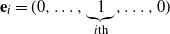 $\textbf{e}_i=(0,\ldots,\underbrace{1}_{i\textrm{th}},\ldots,0)$
for
 $1\leq i\leq d$
. From now on, for any
 $\textbf{x} \in \Delta_d$
, we set
 $x_0= 1-\vert \textbf{x}\vert$
; we have that
 $\textbf{x}= x_0 \textbf{e}_0+x_1 \textbf{e}_1+\cdots + x_d \textbf{e}_d$
with
 $x_i \geq 0$
and
 $x_0+\cdots +x_d=1$
.
We consider the Markov chain
 $(Z_n)_{n\ge 0}$
on the simplex
 $\Delta_d$
corresponding to the successive positions of the robot, according to the following rules:
-
• The robot is put randomly at a point
$Z_0$
in
$\Delta_d$
. -
• If, at time
$n \ge0$
, it is located at
$Z_n=\textbf{x}\in \Delta_d$
, then it chooses the vertex
$\textbf{e}_i$
,
$0\leq i\leq d$
, with probability
$p_i(\textbf{x})$
for the next moving direction and uniformly randomly moves to some point on the open line segment
$(\textbf{x}, \textbf{e}_i)\,{:}\,{\raise-1.5pt{=}}\, \{t\textbf{x} + (1-t)\textbf{e}_i\mid t\in (0, 1)\}$
.



We assume that the functions
 $p_i$
,
 $0\leq i\leq d$
, are continuous and non-negative on
 $\Delta_d$
and satisfy
 ${\sum_{i=0}^n p_i(\textbf{x}) =1}$
for any
 $\textbf{x} \in \Delta_d$
.
Let us make this description more rigorous. For any
 $ i=0, \ldots, d$
and
 $\textbf{x} \in \Delta_d$
, denote by
 $U_i(\textbf{x},\cdot)$
the uniform distribution on
 $(\textbf{x}, \textbf{e}_i)$
; it is defined on open intervals
 $(\textbf{y}_1,\textbf{y}_2) \subset (\textbf{x}, \textbf{e}_i)$
as
 $U_i(\textbf{x}, (\textbf{y}_1,\textbf{y}_2)) \,{:}\,{\raise-1.5pt{=}}\, |t(\textbf{x},\textbf{y}_2,\textbf{e}_i)-t(\textbf{x},\textbf{y}_1,\textbf{e}_i)|$
, where the real number
 $t = t(\textbf{x},\textbf{y},\textbf{e}_i)\in (0, 1)$
solves the equality
 $\textbf{y} = t \textbf{x} + (1-t) \textbf{e}_i$
. The one-step transition probability function P of
 $(Z_n)_{n\ge 0}$
is
 \begin{equation}P(\textbf{x},\textrm{d}\textbf{y})= \sum_{i=0}^d p_i(\textbf{x}) U_i(\textbf{x}, \textrm{d}\textbf{y}), \qquad \textbf{x} \in \Delta_d.\end{equation}
We illustrate this setting in
 $\Delta_2$
in Figure 1.
The Diaconis–Freedman chain in
 $\Delta_2$
.

We want to classify the invariant probability measures of the chain
 $(Z_n)_{n\ge 0}$
and to describe its behavior as
 $n \to +\infty$
. Our approach is based on the description of the spectrum, on some suitable space (to be specified), of the operator corresponding to the one-step transition probability function P, also denoted by P. Let us first introduce this transition operator.
We denote by
 $\textrm{d}\textbf{x}$
the Lebesgue measure on
 $\Delta_d$
and by
 $\mathbb{L}^{\infty}(\Delta_d)$
the space of all bounded Lebesgue-measurable functions
 $f \colon \Delta_d \to \mathbb{C}$
; the dual space of
 $\mathbb{L}^{\infty}(\Delta_d)$
with respect to the Lebesgue measure is
 $\mathbb{L}^1(\Delta_d,\textrm{d}\textbf{x})$
, the space of Lebesgue-measurable functions from
 $\Delta_d$
to
 $\mathbb{C}$
which are integrable with respect to
 $\textrm{d}\textbf{x}$
. The spaces
 $\mathbb{L}^{\infty}(\Delta_d)$
and
 $\mathbb{L}^1(\Delta_d,\textrm{d}\textbf{x})$
are Banach spaces, endowed respectively with the norms
 $\Vert f\Vert_\infty \,{:}\,{\raise-1.5pt{=}}\, \sup_{\textbf{x}\in\Delta_d} |f(\textbf{x})|$
and
 $\Vert g\Vert_1 \,{:}\,{\raise-1.5pt{=}}\, \int_{\Delta_d} |g(\textbf{x})| \, \textrm{d}\textbf{x}$
.
We also denote by
 $Den(\Delta_d,\textrm{d}\textbf{x})=\{g\in \mathbb{L}^1(\Delta_d,\textrm{d}\textbf{x})\;:\;g\ge 0 \text{ and } \int_{\Delta_d}g(\textbf{x}) \, \textrm{d}\textbf{x} = 1\}$
the space of all probability densities on
 $\Delta_d$
with respect to the reference Lebesgue measure
 $\textrm{d}\textbf{x}$
. The set
 $(Den(\Delta_d,\textrm{d}\textbf{x}),d)$
is a complete metric space for the distance
 $d(f,g) \,{:}\,{\raise-1.5pt{=}}\,\Vert f-g\Vert_1$
; furthermore,
 $Den(\Delta_d,\textrm{d}\textbf{x})$
is a non-empty closed convex subset of the Banach space
 $\mathbb{L}^1(\Delta_d, \textrm{d}\textbf{x})$
, and it contains the constant function
 $g(\textbf{x}) \equiv d !$
.
The transition operator of the chain
 $(Z_n)_{n\ge 0}$
is defined by
 \begin{align*} P \colon \mathbb{L}^{\infty}(\Delta_d) \rightarrow \mathbb{L}^{\infty}(\Delta_d) , \qquad f \mapsto\left(Pf\;:\;\textbf{x}\to \int_{\Delta_d} f(\textbf{y})P(\textbf{x},\textrm{d}\textbf{y})\right).\end{align*}
Its dual operator
 $P^* \colon \mathbb{L}^1(\Delta_d, \textrm{d}\textbf{x}) \to \mathbb{L}^1(\Delta_d, \textrm{d}\textbf{x})$
with respect to the Lebesgue measure is defined by
 $\int_{\Delta_d} Pf(\textbf{x})g(\textbf{x}) \, \textrm{d}\textbf{x} = \int_{\Delta_d} f(\textbf{x}) P^*g(\textbf{x}) \, \textrm{d}\textbf{x}$
.
Let us be explicit about the form of these two operators.
Lemma 2.1. Let P be the transition operator of
 $(Z_n)_{n\ge 0}$
, acting on
 $\mathbb{L}^\infty(\Delta_d)$
, and
 $P^*$
its dual operator on
 $\mathbb{L}^1(\Delta_d, \textrm{d}\textbf{x})$
. Then, for any
 $f \in \mathbb{L}^\infty(\Delta_d) $
and
 $\textbf{x} \in \Delta_d$
,
 \begin{equation}Pf(\textbf{x}) = \sum_{i=0}^d p_i(\textbf{x}) \int_0^1 f(t\textbf{x} + (1-t)\textbf{e}_i) \, \textrm{d} t ,\end{equation}
and, for any
 $g \in \mathbb{L}^1(\Delta_d, \textrm{d}\textbf{x}) $
and
 $\textbf{y} \in \Delta_d$
,
 \begin{align} P^*g(\textbf{y}) & = \sum_{i=0}^d \int_{1-y_i}^{1} t^{-d} G_i\bigg(\frac{1}{t}\textbf{y} + \bigg(1-\frac{1}{t}\bigg)\textbf{e}_i\bigg) \, \textrm{d} t \nonumber \\[5pt] & = \sum_{i=0}^d \int_{1}^{\frac{1}{1-y_i}} s^{d-2} G_i\bigg(s\textbf{y} + \bigg(1-s\bigg)\textbf{e}_i\bigg) \, \textrm{d} s ,\end{align}
where
 $G_i(\textbf{y}) = g(\textbf{y}) p_i(\textbf{y})$
.
Proof. The equality (2.1) yields
 \begin{align*}Pf(\textbf{x}) = \int_{\Delta_d} f(\textbf{y})P(\textbf{x},\textrm{d}\textbf{y}) & = \sum_{i=0}^d p_i(\textbf{x}) \int_{(\textbf{x}, \textbf{e}_i)} f(\textbf{y}) U_i(\textbf{x}, \textrm{d}\textbf{y}) \\[5pt] &= \sum_{i=0}^d p_i(\textbf{x}) \int_0^1 f(t\textbf{x} + (1-t)\textbf{e}_i) \, \textrm{d} t. \end{align*}
For the computation of
 $P^*$
, we assume
 $d=2$
; the same argument holds for any d. For all
 $f\in \mathbb{L}^{\infty}(\Delta_d)$
and
 $g\in \mathbb{L}^1(\Delta_d, \textrm{d}\textbf{x})$
,
 \begin{align*}\int_{\Delta_2} f(\textbf{x}) P^*g(\textbf{x}) \, \textrm{d}\textbf{x} &= \int_{\Delta_2} Pf(\textbf{x})g(\textbf{x}) \, \textrm{d}\textbf{x} \\[5pt] &= \sum_{i=0}^2 \int_{\Delta_2}\bigg( p_i(\textbf{x}) \int_0^1 f(t\textbf{x} + (1-t)\textbf{e}_i) \, \textrm{d} t \bigg) g(\textbf{x}) \, \textrm{d}\textbf{x} \\[5pt] &= \sum_{i=0}^2 \int_{\Delta_2}\bigg( G_i(\textbf{x}) \int_0^1 f(t\textbf{x} + (1-t)\textbf{e}_i) \, \textrm{d} t \bigg) \textrm{d}\textbf{x}.\end{align*}
Let us detail the computation of the term
 $\int_{\Delta_2}\Big( G_0(\textbf{x}) \int_0^1 f(t\textbf{x}) \, \textrm{d} t \Big) \, \textrm{d}\textbf{x}$
which corresponds to
 $i = 0$
; the same calculation holds for the other terms:
 \begin{align*}\int_{\Delta_2} \!\! \bigg( G_0(\textbf{x}) \int_0^1 \!\! f(t\textbf{x}) \, \textrm{d} t \bigg) \, \textrm{d}\textbf{x} &= \int_{0}^1 \bigg[\int_0^{1-x_1} \bigg( G_0(\textbf{x}) \int_0^1 f(t\textbf{x}) \, \textrm{d} t \bigg) \, \textrm{d} x_2 \bigg] \, \textrm{d} x_1\\[5pt] &= \int_{0}^1 \bigg[ \int_0^{1} \bigg( \int_0^{1-x_1} G_0(\textbf{x})f(t\textbf{x}) \, \textrm{d} x_2 \bigg) \, \textrm{d} t \bigg] \, \textrm{d} x_1 \\[5pt] &= \int_{0}^1 \bigg[ \int_0^{1} \bigg( \int_0^{1-x_1} G_0(\textbf{x})f(t\textbf{x}) \, \textrm{d} x_2 \bigg) \, \textrm{d} x_1 \bigg] \, \textrm{d} t \\[5pt] & \stackrel{y_2=tx_2}{=} \!\!\! \int_{0}^1 \! \bigg[ \int_0^{1} \!\! \bigg( \int_0^{(1-x_1)t} \!\!\! G_0\bigg(x_1,\frac{y_2}{t}\bigg)f(tx_1, y_2) \frac{\textrm{d} y_2}{t} \bigg) \textrm{d} x_1 \bigg] \textrm{d} t \\[5pt] & \stackrel{y_1=tx_1}{=} \!\!\! \int_{0}^1 \bigg[ \int_0^{t} \!\! \bigg( \int_0^{t-y_1} \!\!\! G_0\bigg(\frac{y_1}{t},\frac{y_2}{t}\bigg)f(y_1, y_2) \frac{\textrm{d} y_2}{t} \bigg) \frac{\textrm{d} y_1}{t} \bigg] \, \textrm{d} t \\[5pt] &= \int_{0}^1 \bigg[ \int_{y_1}^{1} \bigg( \int_0^{t-y_1} \frac{1}{t^2} G_0\bigg(\frac{y_1}{t},\frac{y_2}{t}\bigg)f(y_1, y_2) \, \textrm{d} y_2 \bigg) \, \textrm{d} t \bigg] \, \textrm{d} y_1 \\[5pt] &= \int_{0}^1 \! \bigg[ \int_{0}^{1-y_1} \!\! \bigg( \int_{y_1+y_2}^{1} \! \frac{1}{t^2} G_0\bigg(\frac{y_1}{t},\frac{y_2}{t}\bigg)f(y_1, y_2) \, \textrm{d} t \bigg) \, \textrm{d} y_2 \bigg] \, \textrm{d} y_1 \\[5pt] &= \int_{\Delta_2} f(\textbf{y}) \bigg( \int_{1-y_0}^{1} t^{-2} G_0\bigg(\frac{1}{t} \textbf{y}\bigg) \, \textrm{d} t \bigg) \, \textrm{d} \textbf{y}.\end{align*}
Similarly,
 \begin{equation*} \int_{\Delta_2}\bigg( G_i(\textbf{x}) \int_0^1 f(t\textbf{x} + (1-t)\textbf{e}_i) \, \textrm{d} t \bigg) \, \textrm{d} \textbf{x}= \int_{1}^{\frac{1}{1-y_i}} G_i\big(s\textbf{y} + (1-s)\textbf{e}_i\big) \, \textrm{d} s\end{equation*}
for
 $i=1, 2$
, and (2.3) follows.
Remark 2.1. In dimension
 $d=1$
, Lemma 2.1 is still valid and corresponds to the expression for
 $P^*$
given in [Reference Ladjimi and Peigné20]:
 \begin{equation*} P^*g(y) = \int_{1-y}^{1} \!\!\!\! t^{-1} G_1 \bigg( \frac{1}{t}y + \bigg( 1-\frac{1}{t} \bigg) \bigg) \textrm{d} t + \int_{y}^{1} \!\!\! t^{-1} G_0\bigg(\frac{1}{t}y\bigg) \textrm{d} t = \int_0^y \frac{G_1(s)}{1-s} \textrm{d} s + \int_{y}^1 \frac{G_0(s)}{s} \textrm{d} s.\end{equation*}
Let us summarize some simple properties of P and
 $P^*$
.
Proposition 2.1.
-
(a) The operator P is a Markov operator on
$\mathbb{L}^\infty(\Delta_d)$
, i.e. -
-
(i)
$Pf \ge 0$
whenever
$f\in \mathbb{L}^\infty(\Delta_d)$
and
$f\ge 0$
; -
(ii)
$P1=1$
.
In particular,
$\Vert Pf\Vert_\infty \le \Vert f\Vert_\infty$
for any
$f\in \mathbb{L}^\infty(\Delta_d)$
. Furthermore, P is a Feller operator on
$\Delta_d$
, i.e.
$Pf \in C(\Delta_d)$
for all
$f\in C(\Delta_d)$
. -
-
(c)
$P^*$
acts on
$\mathbb{L}^1(\Delta_d,\textrm{d}\textbf{x})$
and, for any non-negative function
$g\in \mathbb{L}^1(\Delta_d,\textrm{d}\textbf{x})$
,
$P^*g \ge 0$
and
$\Vert P^*g\Vert _1 =\Vert g\Vert _1$
. Furthermore,
$P^*$
acts on
$\textit{Den}(\Delta_d,\textrm{d}\textbf{x})$
, i.e.
$P^* \colon \textit{Den}(\Delta_d,\textrm{d}\textbf{x}) \to \textit{Den}(\Delta_d,\textrm{d}\textbf{x})$
and, for all
$ g_1\ne g_2\in \textit{Den}(\Delta_d,\textrm{d}\textbf{x})$
,
(2.4)
\begin{equation} \Vert P^*g_1-P^*g_2\Vert_1 <\Vert g_1-g_2\Vert_1. \end{equation}







Proof. The properties of P are quite obvious; in particular, the fact that P is a Feller operator is easily checked from the representation (2.2) of P. Similarly, the first properties of
 $P^*$
follow from the definition.
To establish (2.4), we fix
 $ g_1\ne g_2\in Den(\Delta_d,\textrm{d}\textbf{x})$
and set
 $h=g_1-g_2$
. We first note from (2.3) that
 $|P^*h| \leq P^*\vert h|$
on
 $\Delta_d$
, which implies
 $\Vert P^*g_1-P^*g_2\Vert_1 = \Vert P^*h\Vert_1 \leq\Vert P^*\vert h\vert \Vert _1=\Vert h\Vert_1 = \Vert g_1-g_2\Vert_1$
. In fact, the inequality above is strict because both functions
 $g_1$
and
 $g_2$
belong to
 $Den(\Delta_d,\textrm{d}\textbf{x})$
. Ad absurdum, let us assume
 $\Vert P^*h\Vert_1=\Vert h \Vert_1$
. This implies
 $\Vert P^*h\Vert_1=\Vert P^*\vert h\vert\Vert_1$
, and hence
 $\vert P^*h(\textbf{x})\vert = P^*(\vert h\vert)(\textbf{x})$
Lebesgue almost surely (a.s.), since
 $\vert P^*h \vert \leq P^*(\vert h\vert) $
on
 $\Delta_d$
. In other words, for Lebesgue almost all
 $\textbf{x}\in \Delta_d$
,
 \begin{multline*} \Bigg\vert \sum_{i=0}^d \int_{1}^{\frac{1}{1-x_i}} s^{d-2} p_i(s\textbf{x} + (1-s )\textbf{e}_i)h(s\textbf{x} + (1-s )\textbf{e}_i) \Bigg\vert \\[5pt] = \sum_{i=0}^d \int_{1}^{\frac{1}{1-x_i}} s^{d-2} p_i(s\textbf{x} + (1-s )\textbf{e}_i)\vert h(s\textbf{x} + (1-s )\textbf{e}_i)\vert. \end{multline*}
Consequently, for
 $i=0, \ldots, d$
, the quantities
 \begin{equation*} \int_{1}^{\frac{1}{1-x_i}} s^{d-2} p_i(s\textbf{x} + (1-s )\textbf{e}_i)h(s\textbf{x} + (1-s )\textbf{e}_i) \end{equation*}
all have the same sign and
 \begin{multline*} \Bigg\vert\int_{1}^{\frac{1}{1-x_i}} s^{d-2} p_i(s\textbf{x} + (1-s )\textbf{e}_i)h(s\textbf{x} + (1-s )\textbf{e}_i) \Bigg\vert \\[5pt] = \int_{1}^{\frac{1}{1-x_i}} s^{d-2} p_i(s\textbf{x} + (1-s )\textbf{e}_i)\vert h(s\textbf{x} + (1-s )\textbf{e}_i)\vert. \end{multline*}
In other words, for Lebesgue almost all
 $\textbf{x}\in \Delta_d$
, setting
 $\textbf{x}_i\,{:}\,{\raise-1.5pt{=}}\, \frac{1}{1-x_i}\textbf{x}+\big(1-\frac{1}{1-x_i}\big)\textbf{e}_i$
for
 $i=0, \ldots, d$
, the functions
 $p_0 h, \ldots, p_d h$
, restricted respectively to
 $[\textbf{x}, \textbf{x}_0], \ldots, [\textbf{x}, \textbf{x}_d]$
, have the same sign. Hence, the functions
 $h p_0, \ldots, hp_d$
have (Lebesgue a.s.) the same sign on
 $\Delta_d$
. Eventually, the equality
 $p_1 +\cdots +p_d =1$
readily implies that the sign of h is Lebesgue a.s. constant on
 $\Delta_d$
. This contradicts the equality
 $h= g_1-g_2$
with
 $g_1, g_2 \in Den(\Delta_d, \textrm{d}\textbf{x})$
and
 $g_1\neq g_2$
.
As a direct consequence of (2.4), we may state the following corollary.
Corollary 2.1. (Uniqueness of the stationary density function) If a stationary density function for the Markov chain
 $(Z_n)_{n\ge 0}$
exists then it is unique.
Proof. Assume that there are two different stationary density functions
 $f\ne g\in Den(\Delta_d,\textrm{d}\textbf{x})$
, i.e.
 $P^* f = f$
and
 $P^*g = g$
. This implies that
 $d(P^*f,P^*g) = d(f,g)$
, in contradiction with (2.4).
Remark 2.2.
-
(a) Although
$(Den(\Delta_d,\textrm{d}\textbf{x}),d)$
is a complete metric space, the operator
$P^*$
is not uniformly contractive, i.e. there is no
$\rho \in [0, 1)$
such that, for any
$f,g \in Den(\Delta_d,\textrm{d}\textbf{x})$
,
$d(P^* f, P^*g) \le \rho d(f,g)$
. Therefore, we cannot apply the Banach fixed point theorem. In [Reference Ramli and Leng29, Proposition 2, pp.988–989], the authors applied the Banach fixed point theorem to prove the existence of the stationary density function, but their argument does not work. A precise proof can be found in [Reference Ladjimi and Peigné20, Theorem 3.1], which covered all cases of
$p_i(\textbf{x})$
in dimension 1. -
(b) Although
$Den(\Delta_d,\textrm{d}\textbf{x})$
is a non-empty closed convex subset in a Banach space
$\mathbb{L}^1(\Delta_d, \textrm{d}\textbf{x})$
, we cannot apply the Browder fixed point theorem, because
$\mathbb{L}^1(\Delta_d, \textrm{d}\textbf{x})$
is not uniformly convex. -
(c) There are many cases of
$p_i(\textbf{x})$
such that there is no stationary density function for the
$(Z_n)_{n\ge 0}$
even in dimension 1: see cases 2 and 3 in [Reference Ladjimi and Peigné20, Theorem 3.1], where the set of invariant probability measures consists of convex combinations of Dirac measures
$\delta_0$
and
$\delta_1$
. It is of interest to find a criteria on the weight functions
$p_i(\textbf{x})$
which ensures the existence (then the unicity) of a stationary density function. This is still an open question (see the last section of the present paper).







3. General framework for iterated function systems with a unique invariant probability measure
In this section we recall some well-known results for iterated function systems and apply them to our model.
The approach we use here is based on the description of the spectrum of the transition operator associated with
 $(X_n)_{n \geq 0}$
; it is totally different from the one used in [Reference Nguyen and Volkov23], based on criteria of ergodicity and stability of stochastic processes due to A. A. Borovkov [Reference Borovkov4]. We shall use the assumption that our weight functions
 $p_i$
are Hölder, and there is at least one of these functions with full support. This assumption and Assumption 2.2(ii) in [Reference Nguyen and Volkov23] cannot be compared. Therefore, our Theorem 3.4 and their Theorem 2.4 cannot be compared, although their Assumptions 2.2(i) and (iii) for
 $\xi$
cover ours for
 $\xi = U(0, 1)$
. Moreover, the main interest is its flexibility: indeed, it allows us to study the case when several invariant probability measures exist (see Section 5).
3.1. Iterated function systems with place-independent probabilities
Let (E, d) be a compact metric space and denote by
 $\displaystyle \mathbb{L} \textrm{ip}(E, E) $
the space of Lipschitz-continuous functions from E to E, i.e. functions
 $T \colon E\to E$
such that
 \begin{equation*} [T]\,{:}\,{\raise-1.5pt{=}}\, \sup_{\stackrel{x, y\in E}{x\neq y}} \frac{d( T(x),T(y))}{d(x,y)} < \infty.\end{equation*}
Let
 $(T_n)_{n \geq 1}$
be a sequence of i.i.d. random functions defined on a probability space
 $(\Omega, \mathcal T, \mathbb{P})$
with values in
 $\mathbb{L} \textrm{ip}(E, E)$
and common distribution
 $\mu$
. We consider the Markov chain
 $(X_n)_{n \geq 0} $
on E defined, for any
 $n\geq 0$
, by
 \begin{equation}X_{n+1}\,{:}\,{\raise-1.5pt{=}}\, T_{n+1}(X_n),\end{equation}
where
 $X_0$
is a fixed random variable with values in E. We say that the chain
 $(X_n)_{n \geq 0} $
is generated by the iterated function system
 $(T_n)_{n \geq 1}$
. Notice that
 $X_n = T_n\circ\cdots \circ T_1(X_0)$
; it thus corresponds to the forward iterations of the function system
 $(T_n)_{n \geq 1}$
. The stochastic behavior of
 $(X_n)_{n \geq 0}$
is related to the contraction properties of the backward iterations
 $T_1\circ\cdots \circ T_n $
of the function system
 $(T_n)_{n \geq 1}$
, which usually behave more nicely.
The transition operator Q of
 $(X_n)_{n \geq 0}$
is defined, for any bounded Borel function
 $\varphi \colon E \to \mathbb{C}$
and any
 $x\in E$
, by
 $ Q\varphi(x) \,{:}\,{\raise-1.5pt{=}}\, \int_{\mathbb{L} \textrm{ip}(E, E)} \varphi(T(x)) \mu(\textrm{d}T)$
. The chain
 $(X_n)_{n \geq 0} $
has the ‘Feller property’, i.e. the operator Q acts on the space
 $C(E, \mathbb{C})$
of continuous functions from E to
 $\mathbb{C}$
. The maps
 $T_n$
being Lipschitz continuous on E, the operator Q also acts on the space
 $\mathbb{L} \textrm{ip}(E, \mathbb{C})$
of Lipschitz-continuous functions from E to
 $\mathbb{C}$
, and more generally on the space
 $ \mathcal H_\alpha (E, \mathbb{C})$
,
 $0<\alpha \leq 1$
, of
 $\alpha$
-Hölder-continuous functions from E to
 $\mathbb{C}$
defined by
 $\mathcal H_\alpha (E, \mathbb{C})\,{:}\,{\raise-1.5pt{=}}\, \{f\in C(E, \mathbb{C})\mid \Vert f\Vert_\alpha\,{:}\,{\raise-1.5pt{=}}\, \Vert f\Vert_\infty +m_\alpha(f) <+\infty\}$
, where
 \begin{equation*} m_\alpha(f) \,{:}\,{\raise-1.5pt{=}}\, \sup_{\stackrel{x, y \in E}{x\neq y}} \frac{\vert f(x)-f(y)\vert}{d(x,y)^\alpha} < \infty. \end{equation*}
Endowed with the norm
 $\Vert \cdot \Vert_\alpha$
, the space
 $\mathcal H_\alpha (E, \mathbb{C})$
is a Banach space.
The behavior of the chain
 $(X_n)_{n \geq 0} $
is closely related to the spectrum of the restriction of Q to these spaces. Under some ‘contraction in mean’ assumption on the
 $T_n$
, the restriction of Q to
 $\mathcal H_\alpha (E, \mathbb{C})$
satisfies some spectral gap property. We first cite the following result from [Reference Ladjimi and Peigné20, Proposition 2.1].
Theorem 3.1. ([Reference Ladjimi and Peigné20].) Assume that there exists
 $\alpha \in (0, 1]$
such that
 \begin{equation} r\,{:}\,{\raise-1.5pt{=}}\, \sup_{\stackrel{x, y \in E}{x\neq y}}\int_{\mathbb{L}\textrm{ip}(E, E)}\biggl(\frac{ d(T(x),T(y))}{d(x, y)}\biggr)^\alpha \mu(\textrm{d}T) <1.\end{equation}
Then, there exists on E a unique Q-invariant probability measure
 $\nu$
. Furthermore, there exist constants
 $\kappa >0$
and
 $\rho \in (0, 1)$
such that, for all
 $\varphi\in \mathcal H_\alpha (E, \mathbb{C})$
,
 $\Vert Q^n\varphi -\nu(\varphi)\Vert_\alpha \leq \kappa \rho^n\Vert \varphi \Vert_\alpha$
.
Remark 3.1. In the theory of random iterative function systems, it is common to assume contraction in mean in the form
 \begin{equation*} \mathbb{E}\Bigg(\log\sup_{\stackrel{x, y \in E}{x\neq y}}\frac{d(T(x), T(y))}{d(x, y)}\Bigg)<0 , \end{equation*}
which is secured, for instance, by
 \begin{equation*} \mathbb{E}\Bigg(\sup_{\stackrel{x, y \in E}{x\neq y}}\frac{d(T(x), T(y))}{d(x, y)}\Bigg)^\alpha<1. \end{equation*}
The log-contraction condition instead of this last, more restrictive, contraction condition is in fact an improvement of a cosmetic nature, since cases when log-contraction conditions are fulfilled but average contraction conditions are not typically indicate that a change of metric is appropriate (see [Reference Stenflo31] for more details). Notice also that the condition (3.2) (see also condition H1 in Theorem 3.3) is less restrictive, with the supremum put out of the expectation; it already appeared as the ‘global average condition’ in [Reference Stenflo31] and references therein.
3.1.1. Application to the Diaconis–Freedman chain for p fixed in
$\Delta_d$

We assume
 $p_i(\textbf{x}) = p_i$
for all
 $i=0,\ldots, d$
. This puts the Diaconis–Freedman chain into the framework of iterated random functions as follows. For each
 $i=0,\ldots, d$
and
 $t\in [0, 1]$
, we set
 $H_i(t,\cdot) \colon \Delta_d \to \Delta_d, \textbf{x} \mapsto t\textbf{x} + (1-t)\textbf{e}_i$
as an affine transformation; these functions
 $H_i(t, \cdot)$
belong to the space
 $\mathbb{L} \textrm{ip}(\Delta_d, \Delta_d)$
of Lipschitz-continuous functions from
 $\Delta_d$
to
 $\Delta_d$
, with Lipschitz coefficient
 $m(H_i(t, \cdot))=t$
. Then, we consider the probability measure
 $\mu$
on
 $\mathbb{L} \textrm{ip}(\Delta_d, \Delta_d)$
defined by
 \begin{equation}\mu(\textrm{d} T) \,{:}\,{\raise-1.5pt{=}}\, \sum_{i=0}^d p_i \int_{0}^1 \delta_{H_i(t,\cdot)}(\textrm{d} T) \, \textrm{d} t,\end{equation}
where
 $\delta_T$
is the Dirac mass at T. Equation (2.2) may be rewritten as: for all
 $f \in \mathbb{L}^{\infty}(\Delta_d)$
and
 $\textbf{x} \in \Delta_d$
,
 $Q f(\textbf{x}) = \int_{\mathbb{L} \textrm{ip}(\Delta_d, \Delta_d)} f(T(\textbf{x}))\mu(\textrm{d} T)$
. Hence, the Diaconis–Freedman chain
 $(Z_n)_{n \geq 0}$
on
 $\Delta_d$
is generated by the iterated function system
 $(T_n)_{n \geq 1}$
in the sense of (3.1), where
 $(T_n)_{n \geq 1}$
is a sequence of i.i.d. random functions with common distribution
 $\mu$
defined by (3.3).
Theorem 3.2. If
 $p_i(\textbf{x}) = p_i$
for all
 $i=0,\ldots, d$
, then the Diaconis–Freedman chain in
 $\Delta_d$
admits a unique P-invariant probability measure
 $\nu$
on
 $\Delta_d$
. Furthermore, for any
 $\alpha \in (0, 1]$
, there exist constants
 $\kappa>0$
and
 $\rho\in (0, 1)$
depending on
 $\alpha$
such that, for any
 $\varphi\in \mathcal H_\alpha (\Delta_d, \mathbb{C}) $
and
 $ \textbf{x} \in \Delta_d$
,
 $\big\vert Q^n\varphi(\textbf{x})-\nu(\varphi)\big\vert \leq \kappa \rho^n \Vert \varphi\Vert_\alpha$
.
Proof. This is a direct consequence of Theorem 3.1, because, for all
 $\alpha \in (0, 1]$
, we have
 \begin{align*} \quad\qquad\qquad r=\sup_{\stackrel{\textbf{x}, \textbf{y} \in \Delta_d}{\textbf{x}\neq \textbf{y}}}\int_{\mathbb{L} \textrm{ip}(\Delta_d, \Delta_d)}\biggl(\frac{ |T(\textbf{x})-T(\textbf{y})|}{|\textbf{x}- \textbf{y}|}\biggr)^\alpha \mu(\textrm{d}T) &\leq \sum_{i=0}^d p_i \int_0^1 m(H_i(t,\cdot)) ^\alpha \textrm{d}t \\[5pt] &= \int_0^1 t^\alpha \textrm{d}t=\frac{1}{1+\alpha} <1.\end{align*}
Remark 3.2. The unique P-invariant probability measure
 $\nu$
is usually nothing but the Dirichlet distribution
 $Dir[ \theta_0,\ldots, \theta_k ]$
, as will be shown later. If
 $\theta_i >0$
for all
 $i=0,\ldots, k$
, we have a unique invariant probability density which is the Dirichlet density. Otherwise, the Dirichlet distribution is singular and can be understood in the sense of [Reference Ferguson9, p. 211], [Reference Ghosh and Ramamoorthi10, Definition 3.1.1, p. 89], or [Reference Jost, Le and Tran16, Definition 4.2].
3.2. Iterated function systems with place-dependent probabilities
In this subsection we extend the measure
 $\mu$
to a collection
 $(\mu_x)_{x \in E}$
of probability measures on
 $\mathbb{L} \textrm{ip}(E,E)$
, depending continuously on x. We consider the Markov chain
 $(X_n)_{n \geq 0}$
on E whose transition operator Q is given, for any bounded Borel function
 $\varphi\;:\;E \to \mathbb{C}$
and any
 $x\in E$
, by
 $Q\varphi(x)= \int_{\mathbb{L} \textrm{ip}(E, E)} \varphi(T(x)) \mu_x(\textrm{d}T)$
. First, we introduce the following definition.
Definition 3.1. A sequence
 $(\xi_n)_{n \geq 0}$
of continuous functions from E to E is a contracting sequence if there exists
 $x_0 \in E$
such that, for all
 $x \in E$
,
 $\lim_{n \to +\infty} \xi_n(x)= x_0$
.
We cite the following result from [Reference Ladjimi and Peigné20, Proposition 2.2].
Theorem 3.3. ([Reference Ladjimi and Peigné20].) Assume that there exists
 $\alpha \in (0, 1]$
such that
-
H1
$r\,{:}\,{\raise-1.5pt{=}}\,\displaystyle \sup_{\stackrel{x, y \in E}{x\neq y}}\int_{\mathbb{L}\textrm{ip}(E, E)}\biggl(\frac{d(T(x), T(y))}{d(x, y)}\biggr)^\alpha\mu_x(\textrm{d}T) <1$
; -
H2
$R_\alpha\,{:}\,{\raise-1.5pt{=}}\, \displaystyle \sup_{\stackrel{x, y \in E}{x\neq y}}\frac{\vert \mu_x-\mu_y\vert_\textrm{ TV }}{d (x, y)^\alpha}<+\infty$
, where
$\vert \mu_x-\mu_y\vert_\textrm{TV}$
is the total variation distance between
$\mu_x$
and
$\mu_y$
; -
H3 there exist
$\delta >0$
and a probability measure
$\mu$
on E such that -
-
(i) for all
$x \in E$
,
$\mu_x\geq \delta \mu$
; -
(ii) the closed semi-group
$T_\mu$
generated by the support
$S_\mu$
of
$\mu$
possesses a contracting sequence.
-


Then, there exists on E a unique Q-invariant probability measure
 $\nu$
. Furthermore, for some constants
 $\kappa >0$
and
 $\rho \in (0, 1)$
, for any
 $\varphi \in \mathcal H_\alpha(E)$
and
 $x \in E$
,
 $\vert Q^n\varphi(x)-\nu(\varphi)\vert \leq \kappa\rho^n\Vert \varphi\Vert_\alpha$
.
Let us now apply this statement to the Diaconis–Freedman chain on
 $\Delta_d$
. For each
 $\textbf{x}\in \Delta_d$
, we define a space-dependent probability measure
 $\mu_{\textbf{x}}$
on
 ${\mathbb{L} \textrm{ip}(\Delta_d,\Delta_d)}$
by
 \begin{equation*}\mu_{\textbf{x}}(\textrm{d} T) \,{:}\,{\raise-1.5pt{=}}\, \sum_{i=0}^d p_i(\textbf{x}) \int_{0}^1 \delta_{H_i(t,\cdot)}(\textrm{d} T) \, \textrm{d} t,\end{equation*}
where
 $\delta_T$
is the Dirac mass at T. With this collection
 $(\mu_{\textbf{x}})_{\textbf{x} \in \Delta_d}$
of probability measures, the Diaconis–Freedman chain falls within the scope of Theorem 3.3.
Theorem 3.4. Assume that
-
(i) for all
$j=0,\ldots, d$
, the functions
$p_j$
belong to
$\mathcal H_\alpha (\Delta_d, \mathbb{C})$
; -
(ii) there exists
$i\in \{0,\ldots, d\}$
such that
$\delta_i\,{:}\,{\raise-1.5pt{=}}\,\min_{\textbf{x} \in \Delta_d}p_i(\textbf{x}) > 0$
.


Then, the Diaconis–Freedman chain in
 $\Delta_d$
has a unique P-invariant probability measure
 $\nu$
on
 $ \Delta_d$
. Furthermore, there exist constants
 $\kappa >0$
and
 $\rho \in (0, 1)$
such that, for any
 $\varphi\in \mathcal H_\alpha (\Delta_d, \mathbb{C})$
and
 $\textbf{x} \in \Delta_d$
,
 $\vert P^n\varphi(\textbf{x})-\nu(\varphi)\vert \leq \kappa \rho^n \Vert \varphi\Vert_\alpha$
.
Proof. This is a direct consequence of Theorem 3.3 since conditions H1–H3 hold in this context:
-
H1 For any
$\textbf{x} \ne \textbf{y} \in \Delta_d$
,
\begin{align*} \int_{\mathbb{L} \textrm{ip}(\Delta_d, \Delta_d)} \bigg(\frac{|T(\textbf{x})-T(\textbf{y})|}{|\textbf{x}-\textbf{y}|}\bigg)^{\alpha} \mu_{\textbf{x}}(\textrm{d} T) &= \sum_{i=0}^d p_i(\textbf{x}) \int_0^1 \bigg(\frac{|H_i(t,\textbf{x})-H_i(t,\textbf{y})|}{|\textbf{x}-\textbf{y}|}\bigg)^{\alpha} \, \textrm{d} t \\[5pt] &= \frac{1}{1+\alpha} < 1. \end{align*}
-
H2 For any
$\textbf{x} \ne \textbf{y} \in \Delta_d$
and any Borel set
$A \subseteq \mathbb{L} \textrm{ip}(\Delta_d,\Delta_d)$
,
\begin{align*} \frac{|\mu_{\textbf{x}}(A)-\mu_{\textbf{y}}(A)|}{|\textbf{x}-\textbf{y}|^{\alpha}} &\le \sum_{i=0}^d \frac{|p_i(\textbf{x})-p_i(\textbf{y})|}{|\textbf{x}-\textbf{y}|^{\alpha}} {\int_{0}^1 \delta_{H_i(t,\cdot)}(A) \, \textrm{d} t} \\[5pt] & \le \sum_{i=0}^d m_{\alpha}(p_i) < \infty.\end{align*}
-
H3 Set
$\mu(\textrm{d} T) \,{:}\,{\raise-1.5pt{=}}\, \int_0^1 \delta_{H_i(t,\cdot)}(\textrm{d} T) \, \textrm{d} t$
; then, for all
$\textbf{x}\in \Delta_d$
,
Moreover, the constant function
\begin{equation*}\mu_{\textbf{x}}(\textrm{d} T) \ge p_i(\textbf{x}) \int_{0}^1 \delta_{H_i(t,\cdot)}(\textrm{d} T) \, \textrm{d} t \ge \delta \mu(\textrm{d} T).\end{equation*}
$\textbf{x}\mapsto 0$
belongs to the support of
$\mu$
so that the semigroup
$T_{\mu}$
contains a contracting sequence with limit point 0.







We emphasize that under conditions H1–H3, the eigenvalue 1 is simple and is the unique eigenvalue of Q with modulus 1; the proof requires precise control of the peripherical spectrum of Q; see the proof of [Reference Ladjimi and Peigné20, Proposition 2.2].
4. Some explicit invariant probability densities
In this section we consider some special cases of weights for which it is possible to compute explicitly the unique invariant probability density. When
 ${d}=1$
, it is known that, when both conditions
 $p_1(0) > 0$
and
 $p_0(1)>0$
hold, there exists a unique invariant probability density of
 $(Z_n)_{n\ge 0}$
given by
 \begin{equation*}g_{\infty}(y) = C\exp \bigg(\int_{1/2}^y \frac{p_1(t)}{1-t} \, \textrm{d} t - \int_{1/2}^y \frac{p_0(t)}{t} \, \textrm{d} t \bigg) ; \end{equation*}
see, for instance, [Reference Ramli and Leng29] or [Reference Ladjimi and Peigné20]. We do not get such a general result when
 $d \geq 2$
, we can do it only in some specific cases. We would also like to emphasize that in [Reference Nguyen and Volkov23], based on Sethuraman’s construction of the Dirichlet distributions [Reference Sethuraman30], the authors also gave general results for the explicit formula of the stationary density in these special cases. Our approach, however, is very natural and worth taking into account.
4.1. The case of constant weights
We first consider the case of constant weights, i.e.
 $p_i(\textbf{x}) = p_i>0$
for all
 $i=0,\ldots, d$
.
Theorem 4.1. If
 $p_i(\textbf{x})=p_i>0$
for all
 $i=0,\ldots,d$
, then the unique invariant probability density
 $ g_\infty $
of
 $(Z_n)_{n\ge 0}$
is the density of the Dirichlet distribution
 $Dir[p_0,\ldots,p_d]$
, i.e.
 \begin{equation*}g_\infty (\textbf{y}) = \frac{1}{\prod_{i=0}^d \Gamma(p_i)} \prod_{i=0}^d y_i^{p_i-1} \textbf{1}_{\mathring \Delta_d }(\textbf{y})\end{equation*}
for any
 $\textbf{y}= (y_1, \ldots, y_d)$
in
 $\Delta_d$
, where
 $y_0 = 1-y_1-\cdots- y_d$
.
Proof. It suffices to prove that
 $g_\infty(\textbf{y})=\prod_{i=0}^d y_i^{\alpha_i}$
with
 $\alpha_i=p_i-1$
is the unique solution of the equation
 $P^*g(\textbf{y}) = g(\textbf{y})$
. Indeed, according to (2.3),
 \begin{align}P^*g_\infty(\textbf{y}) &= \sum_{i=0}^d p_i \int_{1}^{\frac{1}{1-y_i}} s^{d-2} g_\infty\bigg(s\textbf{y} + (1-s)\textbf{e}_i\bigg) \, \textrm{d} s\notag \\[5pt] &= \sum_{i=0}^d p_i \int_{1}^{\frac{1}{1-y_i}} s^{d-2} (sy_i+1-s)^{\alpha_i} \prod_{j\ne i}(sy_j)^{\alpha_j} \, \textrm{d} s\notag\\[5pt] &= \sum_{i=0}^d p_i \int_{1}^{\frac{1}{1-y_i}} s^{d-2+\sum_{j\ne i}\alpha_j} (sy_i+1-s)^{\alpha_i} \frac{g_\infty(\textbf{y})}{y_i^{\alpha_i}}\, \textrm{d} s\notag \\[5pt] &= \sum_{i=0}^d \frac{p_i}{(1-y_i) y_i^{\alpha_i}(1-y_i)^{-2-\alpha_i}} \left(\int_{0}^{y_i}t^{\alpha_i}(1-t)^{-2-\alpha_i}\, \textrm{d} t \right) g_\infty(\textbf{y} ) ,\end{align}
where the last equality follows by using the change of variables
 $t = sy_i+1-s$
and the equality
 $\sum_{j=0}^d \alpha_j = -d$
. Notice that, for
 $i=0, \ldots, d$
and
 $\alpha_i>-1$
,
 \begin{equation*}(1+\alpha_i)\int_{0}^{y_i}t^{\alpha_i}(1-t)^{-2-\alpha_i} \, \textrm{d} t = y_i^{1+\alpha_i}(1-y_i)^{-1-\alpha_i}.\end{equation*}
As a matter of fact, the function
 $ F \colon y_i\mapsto (1+\alpha_i)\int_{0}^{y_i}t^{\alpha_i}(1-t)^{-2-\alpha_i} \, \textrm{d} t - y_i^{1+\alpha_i}(1-y_i)^{-1-\alpha_i}$
satisfies
 $F(0)=0$
and
 $F'(y_i) = 0$
; therefore,
 $F(y_i) \equiv 0$
. Hence, the equality (4.1) yields
 \begin{equation*}P^*g_\infty(\textbf{y}) = \sum_{i=0}^d y_i g_\infty(\textbf{y}) =g_\infty(\textbf{y}).\end{equation*}
The uniqueness stems from Corollary 2.1.
Example 4.1. When
 $d=2$
,
 $p_1= p_2= p_0=1/3$
, the unique invariant probability density is
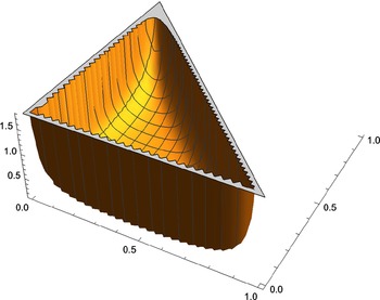
 \begin{equation*}g_{\infty}(\textbf{y}) = \frac{1}{\Gamma(1/3)^3} y_1^{-\frac{2}{3}} y_2^{-\frac{2}{3}}(1-y_1-y_2)^{-\frac{2}{3}} \textbf{1}_{\Delta_2}(\textbf{y}) \end{equation*}
(see Figure 2).
Figure 3 represents random trajectories of
 $(Z_n)_{n\ge 0}$
:
-
• in [0, 1], starting at
$x_0=0.6$
with
$p_1(x)=0.2$
,
$p_0(x) = 0.8$
, in the left panel; -
• in
$\Delta_2$
, starting at
$\textbf{x}_0=(0.3,0.4)$
with
$p_1(\textbf{x}) = 0.5$
,
$p_2(\textbf{x})= 0.2$
,
$p_0(\textbf{x})=0.3$
in the right panel.


They both illustrate the ergodic behavior of the chain.
The density function of the Dirichlet distribution
 $Dir\big[\frac{1}{3},\frac{1}{3},\frac{1}{3}\big]$
.

Left: Random trajectory of
 $Z_n$
in [0,Reference Barnsley, Demko, Elton and Geronimo1] starting at
 $x_0=0.6$
. Right: Random trajectory of
 $Z_n$
in
 $\Delta_2$
starting at
 $\textbf{x}_0=(0.3,0.4)$
.

4.2. The case of affine weights
In this section we present a special case of non-constant weight functions
 $p_i(\textbf{y})$
which yield an explicit form of the unique invariant density function.
Theorem 4.2. Fix positive constants
 $\theta_0, \ldots, \theta_d > 0$
with
 $|\boldsymbol{\theta}| = \theta_0 +\cdots +\theta_d \le 1$
, and assume that, for any
 $i=1, \ldots, d$
and
 $\textbf{x}= (x_1, \ldots, x_d)$
in
 $\Delta_d$
,
 $p_i(\textbf{x}) =\tilde p_i(x_i)\,{:}\,{\raise-1.5pt{=}}\, \theta_i +(1-|\boldsymbol{\theta}| ) x_i$
(which implicitly implies
 $p_0(\textbf{x}) = \tilde p_0(x_0)\,{:}\,{\raise-1.5pt{=}}\,\theta_0 + (1-|\boldsymbol{\theta}|) x_0$
). Then, the unique invariant probability density
 $g_\infty$
of
 $(Z_n)_{n\ge 0}$
is the Dirichlet distribution
 $Dir[\theta_0,\ldots,\theta_d]$
given by
 \begin{equation*}g_\infty(\textbf{y}) = Dir[\theta_0,\ldots,\theta_d](\textbf{y}) = \frac{\Gamma(|\boldsymbol{\theta}|)}{\prod_{i=0}^d \Gamma(\theta_i)}\prod_{i=0}^d y_i^{\theta_i-1}\textbf{1}_{\mathring{\Delta}_d}(\textbf{y}) \end{equation*}
for any
 $\textbf{y}= (y_1, \ldots, y_d)$
in
 $\Delta_d$
, where
 $y_0 = 1-y_1-\cdots- y_d$
.
Proof. Using the same techniques as in the proof of Theorem 4.1, we only need to check that
 \begin{equation*} \frac{\int_0^{y_i} p_i(t) t^{\alpha_i} (1-t)^{|\boldsymbol{\alpha}| -\alpha_i +d-2}\, \textrm{d} t }{y_i^{\alpha_i} (1-y_i)^{|\boldsymbol{\alpha}| -\alpha_i +d-1}} = y_i,\end{equation*}
which can be easily done by a direct calculation.
Remark 4.1.
-
(i) The case when
$|\boldsymbol{\theta}|=1$
corresponds to constant weights. -
(ii) This result has a very close connection to results studied in Wright–Fisher models with mutations (see, for instance, [Reference Hofrichter, Jost and Tran15, Reference Tran, Hofrichter and Jost32, Reference Tran, Hofrichter and Jost33]).

In Figure 4 we simulate random trajectories of
 $(Z_n)_{n\ge 0}$
:
-
• in [0, 1], starting at
$x_0=0.6$
with
$p_1(x)=x$
,
$p_0(x) = 1-x$
in the left panel; -
• in
$\Delta_2$
starting at
$\textbf{x}_0=(0.3,0.4)$
with
$p_1(\textbf{x}) = x_1$
,
$p_2(\textbf{x})= x_2$
,
$p_0(\textbf{x})=1-x_1-x_2$
in the right panel. They both illustrate the absorbing behavior of the chain.


Left: Four random trajectories of
 $Z_n$
in [0,Reference Barnsley, Demko, Elton and Geronimo1] starting at
 $x_0=0.8$
; they will absorb in
 $\{0, 1\}$
. Right: Four random trajectories of
 $Z_n$
in
 $\Delta_2$
starting at
 $\textbf{x}_0=(0.3,0.4)$
; they will absorb in
 $\{\textbf{e}_0, \textbf{e}_2\}$
.

5. Asymptotic behavior of
$(\boldsymbol{Z}_{\boldsymbol{{n}}})_{\boldsymbol{{n}}{\boldsymbol\,\ge\,} \textbf{0}}$

In this section we describe the asymptotic behavior of
 $(Z_n)_{n\ge 0}$
using the notion of minimal P-absorbing compact subsets. First, we establish some properties of the family
 $\mathcal K_m$
of these subsets and propose their classification. By a general results of [Reference Hervé14], this yields the classification of the set of P-invariant probability measures as well as the description of the asymptotic behavior of
 $(Z_n)_{n\ge 0}$
. The classification is complete in
 $\Delta_2$
but partial in
 $\Delta_d$
,
 $d>2$
.
5.1. The set
$\mathcal K_{\boldsymbol{{m}}}$
of minimal P-absorbing compact subsets

Definition 5.1. A non-empty compact subset
 $K\subseteq \Delta_d$
is said to be P-absorbing if, for all
 $\textbf{x} \in K$
,
 \begin{equation*}P(\textbf{x},K^\textrm{c}) \,{:}\,{\raise-1.5pt{=}}\, P\textbf{1}_{K^\textrm{c}}(\textbf{x}) = \sum\limits_{i=0}^d p_i(\textbf{x}) \int_0^1 \textbf{1}_{K^\textrm{c}}(t\textbf{x} + (1-t)e_i)\, \textrm{d} t = 0,\end{equation*}
where
 $K^\textrm{c} = \Delta_d \setminus K$
. It is minimal when it does not contain any proper P-absorbing compact subset.
We denote by
 $\mathcal K_m$
the set of all minimal P-absorbing compact subsets. For any
 $\textbf{x}_0 \in \Delta_d$
and
 $\varepsilon>0$
, we set
 $B_{\varepsilon}(\textbf{x}_0) = \{\textbf{x} \in \Delta_d\;:\;|\textbf{x}-\textbf{x}_0| < \varepsilon\}$
and
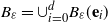 $B_{\varepsilon} = \cup_{i=0}^d B_{\varepsilon}(\textbf{e}_i)$
; Figure 5 shows the domain
 $B_{\varepsilon}(\textbf{e}_i)$
.
The domain
 $B_{\varepsilon}(\textbf{e}_i)$
.

The following rules are useful for describing the minimal P-absorbing sets K.
Proposition 5.1. Given continuous weight functions
 $p_i(\textbf{x})$
on
 $\Delta_d$
, i.e.
 $p_i(\textbf{x}) \ge 0$
for every
 $i=0,\ldots, d$
and
 $\sum_{i=0}^d p_i(\textbf{x})=1$
:
-
(i) If
$K\in \mathcal K_m$
then K contains at least one vertex. -
(ii) If
$K\in \mathcal K_m$
,
$\textbf{e}_i\in K$
, and
$p_i(\textbf{e}_i) =1$
then
$K=\{\textbf{e}_i\}$
. -
(iii) If
$K\in \mathcal K_m$
,
$\textbf{e}_i\in K$
, and
$p_j(\textbf{e}_i) > 0$
for some
$j\ne i$
then
$[\textbf{e}_i,\textbf{e}_j] \subseteq K$
. -
(iv) If
$K\in \mathcal K_m$
and
${p_i}(\textbf{x}) > 0$
for some
$\textbf{x} \in K\setminus\{\textbf{e}_i\}$
then
$[\textbf{e}_i,\textbf{x}] \subseteq K$
.


Proof.
-
(i) Assume that
$\textbf{e}_i \notin K$
for all
$i=0,\ldots, d$
. Since
$K^\textrm{c}$
is open, there exists
$\varepsilon > 0$
such that
$B_{\varepsilon} \subseteq K^\textrm{c}$
. Therefore, for all
$\textbf{x} \in K$
, This contradicts the fact that K is P-absorbing.
\begin{align*} P(\textbf{x},K^\textrm{c}) & = \sum_{i=0}^d p_i(\textbf{x}) \int_0^1 \textbf{1}_{K^\textrm{c}}(t\textbf{x} +(1-t) e_i)\, \textrm{d} t \\[5pt] & \ge \sum_{i=0}^d p_i(\textbf{x}) \int_0^1 \textbf{1}_{B_{\varepsilon}}(t\textbf{x} +(1-t) e_i)\, \textrm{d} t = \sum_{i=0}^d p_i(\textbf{x}) \varepsilon = \varepsilon >0. \end{align*}
-
(ii) It suffices to prove that
$\{\textbf{e}_i\} \in \mathcal K_m$
. This is true because
\begin{equation*} P(\textbf{e}_i, \{\textbf{e}_i\}^\textrm{c}) = \sum\limits_{j\ne i} p_j(\textbf{e}_i) = 0. \end{equation*}
-
(iii) If
$[\textbf{e}_i,\textbf{e}_j] \cap K^\textrm{c}\neq \emptyset$
, then there exist
$\textbf{x}_0 \in [\textbf{e}_i,\textbf{e}_j] \cap K^\textrm{c}$
and
$\varepsilon>0$
such that
$B_{\varepsilon}(\textbf{x}_0) \subseteq K^\textrm{c}$
. Therefore,
$P(\textbf{e}_i,K^\textrm{c}) \ge p_j(\textbf{e}_i) \varepsilon > 0$
, a contradiction. -
(iv) Again, if
$[\textbf{e}_i,\textbf{e}_j] \cap K^\textrm{c}\neq \emptyset$
, then there exist
$\textbf{x}_0 \in [\textbf{e}_i,\textbf{e}_j] \cap K^\textrm{c}$
and
$\varepsilon>0$
such that
$B_{\varepsilon}(\textbf{x}_0) \subseteq K^\textrm{c}$
; hence,
$P(\textbf{x},K^\textrm{c}) \ge p_i(\textbf{x}) \varepsilon > 0$
, which is a contradiction.









This proposition easily yields the classification of
 $\mathcal K_m$
when
 $d=1$
(see [Reference Ladjimi and Peigné20]):
-
(i) If
$p_1(1) <1 $
and
$p_0(0) < 1$
then
$\mathcal K_m = \{[0, 1]\}$
. -
(ii) If
$p_1(1) <1$
and
$p_0(0) = 1$
then
$\mathcal K_m = \{\{1\}\}$
. -
(iii) If
$p_1(1) = 1$
and
$p_0(0) < 1$
then
$\mathcal K_m = \{\{0\}\}$
. -
(iv) If
$p_1(1) = 1$
and
$p_0(0) = 1$
then
$\mathcal K_m = \{\{0\},\{1\}\}$
.



Proposition 5.1 is also sufficient to get the full classification of the set
 $\mathcal K_m$
in
 $\Delta_2$
. In the next two subsections we focus on this classification and the asymptotic behavior of
 $(Z_n)_{n \geq 0}$
in
 $\Delta_2$
. The reader may be easily convinced that similar statements hold in higher dimensions, with technical difficulties we do not want to contend with here; an expanded version of Proposition 5.1 is required when
 $d \geq 3$
.
5.2. Classification of
$\mathcal{K}_{\boldsymbol{{m}}}$
in
$\Delta_2$


We assume
 $d=2$
in this subsection. Unlike the case
 $d=1$
, for the case of
 $d=2$
we need to classify the values of
 $p_i$
not only on the vertices but also on the edges. We denote
 $L_0=\{\textbf{x} \in [\textbf{e}_1,\textbf{e}_2]\;:\;p_0(\textbf{x})>0\}$
,
 $L_1=\{\textbf{x} \in [\textbf{e}_0,\textbf{e}_2]\;:\;p_1(\textbf{x})>0\}$
, and
 $L_2=\{\textbf{x} \in [\textbf{e}_0,\textbf{e}_1]\;:\;p_2(\textbf{x})>0\}$
. Let
 $L^\textrm{c}_0$
(respectively
 $L^\textrm{c}_1$
and
 $L^\textrm{c}_2$
) be the complement of
 $L_0$
(resp.
 $L_1$
and
 $L_2$
) in
 $ [\textbf{e}_1,\textbf{e}_2]$
(resp.
 $[\textbf{e}_0,\textbf{e}_2]$
and
 $[\textbf{e}_0,\textbf{e}_1]$
).
Let us fix
 $K \in \mathcal K_m$
. There are several cases to consider.
5.2.1
$p_0(\textbf{e}_0) = p_1(\textbf{e}_1)=p_2(\textbf{e}_2)=1$

By Proposition 5.1(i), either
 $\textbf{e}_0 \in K$
or
 $\textbf{e}_1 \in K$
or
 $\textbf{e}_2 \in K$
. When
 $\textbf{e}_0\in K$
, Proposition 5.1(ii) implies
 $K=\{\textbf{e}_0\}$
; similarly for
 $\textbf{e}_1$
or
 $\textbf{e}_2$
. Finally,
 $\mathcal K_m = \{\{\textbf{e}_0\},\{\textbf{e}_1\},\{\textbf{e}_2\}\}$
.
5.2.2
$p_0(\textbf{e}_0) = p_1(\textbf{e}_1)=1 $
but
$p_2(\textbf{e}_2)<1$


As above, if
 $\textbf{e}_0\in K$
(resp.
 $\textbf{e}_1\in K$
) then
 $K=\{\textbf{e}_0\}$
(resp.
 $\textbf{e}_1\in K$
). Assume now that
 $\textbf{e}_2\in K$
. Proposition 5.1(iii) implies
 $[\textbf{e}_0,\textbf{e}_2] \subseteq K$
when
 $p_2(\textbf{e}_0) > 0$
and
 $[\textbf{e}_1,\textbf{e}_2] \subseteq K$
when
 $p_2(\textbf{e}_1) > 0$
. Therefore, K contains
 $\textbf{e}_1$
or
 $\textbf{e}_2$
, in contradiction with the minimality of K. Finally,
 $\mathcal K_m = \{\{\textbf{e}_0\},\{\textbf{e}_1\}\}$
.
Similar statements hold when
 $p_0(\textbf{e}_0) = p_2(\textbf{e}_2) =1$
but
 $p_1(\textbf{e}_1) <1$
or
 $p_1(\textbf{e}_1) = p_2(\textbf{e}_2) = 1$
but
 $p_0(\textbf{e}_0) <1$
.
5.2.3
$p_0(\textbf{e}_0) =1$
but
$p_1(\textbf{e}_1), p_2(\textbf{e}_2)<1$


Firstly,
 $\{\textbf{e}_0\}\in \mathcal K_m$
and
 $K=\{\textbf{e}_0\}$
as soon as
 $\textbf{e}_0\in K$
.
Assume now
 $\textbf{e}_0\notin K$
(thus
 $B_{\varepsilon}(\textbf{e}_0) \subseteq K^\textrm{c}$
for some
 $\varepsilon>0$
; see Figure 6) and suppose, for instance,
 $\textbf{e}_1 \in K$
(the same argument holds with
 $\textbf{e}_2$
). Hence,
 $p_0(\textbf{e}_1) = 0$
; indeed, the condition
 $p_0(\textbf{e}_1) > 0$
implies
 $[\textbf{e}_0,\textbf{e}_1] \subseteq K$
, a contradiction. Consequently,
 $p_2(\textbf{e}_1) > 0$
, which implies
 $[\textbf{e}_1,\textbf{e}_2] \subseteq K$
, so
 $p_0(\textbf{e}_2) = 0$
and
 $p_1(\textbf{e}_2) > 0$
. This readily implies that
 $L_0 =\emptyset$
; otherwise,
 $p_0(\textbf{x}_0) > 0$
for some
 $\textbf{x}_0\in [\textbf{e}_1,\textbf{e}_2]$
, and therefore
 $P(\textbf{x}_0, K^\textrm{c}) \ge p_0(\textbf{x}_0) \varepsilon >0$
, contradicting the fact that
 $\textbf{x}_0\in K$
and K is invariant. The equality
 $L_0 =\emptyset$
yields
 $K=[\textbf{e}_1,\textbf{e}_2]$
and
 $\mathcal K_m = \{\{\textbf{e}_0\},[\textbf{e}_1,\textbf{e}_2]\}$
. Finally,
 \begin{equation*}\mathcal K_m =\begin{cases}\{\{\textbf{e}_0\}, [\textbf{e}_1,\textbf{e}_2]\} & \text{ if } L_0=\emptyset , \\[5pt] \{\{\textbf{e}_0\}\} & \text{ otherwise. }\end{cases}\end{equation*}
Domain
 $B_{\varepsilon}(\textbf{e}_0)$
.

Similar statements hold when
 $p_1(\textbf{e}_1)=1$
but
 $p_0(\textbf{e}_0), p_2(\textbf{e}_2)<1$
, or
 $p_2(\textbf{e}_2) =1$
but
 $p_0(\textbf{e}_0), p_1(\textbf{e}_1)<1$
.
5.2.4
$p_0(\textbf{e}_0), p_1(\textbf{e}_1), p_2(\textbf{e}_2)<1$
and
$L_0=\emptyset$


By Proposition 5.1(i), the set K contains at least one of the vertices. Assume, for instance,
 $\textbf{e}_1 \in K$
; thus,
 $p_2(\textbf{e}_1) > 0 $
since
 $L_0=\emptyset$
, which implies
 $[\textbf{e}_1,\textbf{e}_2] \subseteq K$
. The condition
 $L_0=\emptyset$
also implies
 $P(\textbf{x}, [\textbf{e}_1,\textbf{e}_2]^\textrm{c}) = p_0(\textbf{x}) = 0$
for all
 $\textbf{x}\in[\textbf{e}_1,\textbf{e}_2]$
, and finally
 $K=[\textbf{e}_1,\textbf{e}_2]$
. The same conclusion holds when
 $\textbf{e}_2 \in K$
.
Now, the set K cannot contain
 $\textbf{e}_0$
. Otherwise, the condition
 $p_0(\textbf{e}_0)<1$
implies either
 $[\textbf{e}_0, \textbf{e}_1] \subseteq K$
or
 $[\textbf{e}_0, \textbf{e}_2] \subseteq K$
; thus,
 $\textbf{e}_1\in K$
or
 $\textbf{e}_2\in K$
. This yields
 $K=[\textbf{e}_1, \textbf{e}_2]$
, a contradiction. Finally,
 $\mathcal K_m = \{[\textbf{e}_1,\textbf{e}_2]\}$
.
Similar statements hold when
 $L_1=\emptyset$
or
 $L_2=\emptyset$
.
5.2.5
$p_0(\textbf{e}_0), p_1(\textbf{e}_1), p_2(\textbf{e}_2)<1$
and
$L_0, L_1, L_2$
non-empty


In this case we always have
 $\{\textbf{e}_0,\textbf{e}_1,\textbf{e}_2\} \subseteq K$
. Indeed, by Proposition 5.1(i), the set K contains at least one vertex, say
 $\textbf{e}_0 \in K$
; since
 $p_0(\textbf{e}_0) <1$
, it contains one of the two sides
 $[\textbf{e}_0,\textbf{e}_1] $
or
 $[\textbf{e}_0,\textbf{e}_2] $
. Assume
 $[\textbf{e}_0,\textbf{e}_1] \subset K$
(thus
 $\textbf{e}_1\in K$
) and let us check that
 $\textbf{e}_2 \in K$
. Otherwise,
 $B_{\varepsilon}(\textbf{e}_2) \subseteq K^\textrm{c}$
for some
 $\varepsilon>0$
; since
 $L_2$
is a proper subset of
 $[\textbf{e}_0,\textbf{e}_1]$
, there exists
 $\textbf{x}\in [\textbf{e}_0,\textbf{e}_1] \subseteq K$
such that
 $P(\textbf{x},K^\textrm{c}) \ge p_2(\textbf{x})\varepsilon >0$
, a contradiction.
Now, the inclusion
 $\{\textbf{e}_0,\textbf{e}_1,\textbf{e}_2\} \subseteq K$
combined with Proposition 5.1(iv) yields
 $co\{\textbf{e}_0, L_0\} \subseteq K$
,
 $co\{\textbf{e}_1, L_1\} \subseteq K$
, and
 $co\{\textbf{e}_2, L_2\} \subseteq K$
, so that, by the compactness of K,
 \begin{equation}K_0 \,{:}\,{\raise-1.5pt{=}}\, \overline{\textit{co}\{\textbf{e}_0, L_0\} \cup \textit{co}\{\textbf{e}_1, L_1\} \cup \textit{co}\{\textbf{e}_2, L_2\}} \subseteq K.\end{equation}
Next, for all
 $i \in \{0, 1,2\}$
we denote
 $L_i(1) \,{:}\,{\raise-1.5pt{=}}\, \{\textbf{x} \in K_0\;:\;p_i(\textbf{x}) > 0\}$
. It is easy to see that
 $L_i(1) \supseteq L_i$
for all
 $i\in \{0, 1,2\}$
. Then, Proposition 5.1(iv) and the compactness of K yield
 \begin{equation}K_1 \,{:}\,{\raise-1.5pt{=}}\, \overline{\textit{co}\{\textbf{e}_0, L_0(1)\} \cup \textit{co}\{\textbf{e}_1, L_1(1)\} \cup \textit{co}\{\textbf{e}_2, L_2(1)\}} \subseteq K.\end{equation}
We construct by induction a sequence of increasing compact subsets
 $\{K_n\}_{n\ge 0} \subseteq K$
and consider two possibilities: if there is a finite n such that
 $K_n = \Delta_2$
then
 $K =\Delta_2$
; otherwise,
 $K=K_{\infty}\,{:}\,{\raise-1.5pt{=}}\,\overline{\{\cup_{n\ge 0} K_n\}} \subset \Delta_2$
. In this case
 $\mathcal K_m$
consists of a unique minimal P-absorbing compact set,
 \begin{equation*}\mathcal K_m=\begin{cases}\{\Delta_2\} &\text{ if there exists a finite} n \text{such that} K_n=\Delta_2, \\[5pt] \{K_{\infty}\} &\text{ otherwise.}\end{cases}\end{equation*}
We illustrate here two cases when
 $\mathcal K_m = \{K_0\}$
and
 $\mathcal K_m = \{K_1\}$
. If we assume that, for
 $i=0, 1, 2$
,
 \begin{equation}p_i(\textbf{x}) = 0 \text{ for all } \textbf{x} \in \Omega_i\,{:}\,{\raise-1.5pt{=}}\,\{\textbf{y}\in K_0\;:\;[\textbf{y},\textbf{e}_i] \cap K_0^\textrm{c} \ne \emptyset\} ,\end{equation}
then
 $K_1=K_0$
and, by induction,
 $K_{\infty} = K_0$
. Moreover, from (5.3),
 $P(\textbf{x},K_0^\textrm{c}) = 0$
for all
 $\textbf{x}\in K_0$
, and therefore
 $K = K_0$
by the minimality of K and (5.1) (see Figure 7).
 $K_0$
= white domains
 $\cup $
yellow domains =
 $\Delta_2 \setminus$
green domain;
 $K_0^\textrm{c}$
is the green domain;
 $\Omega_1$
,
 $\Omega_2$
, and
 $\Omega_0$
are the yellow domains I,
 $II$
, and
 $III$
respectively.

If we assume now, for
 $i=0, 1, 2$
,
 \begin{equation}p_i(\textbf{x}) = 0 \text{ for all } \textbf{x} \in \Omega_i(1)\,{:}\,{\raise-1.5pt{=}}\,\{ i\textrm{th}\ \text{yellow region}\} ,\end{equation}
then
 $K_1\ne K_0$
,
 $K_2=K_1$
, and iteratively
 $K_{\infty} = K_1$
. Moreover, by (5.4),
 $P(\textbf{x},K_1^\textrm{c}) = 0$
for all
 $\textbf{x}\in K_1$
, and therefore
 $K = K_1$
by the minimality of K and (5.2) (see Figure 8).
 $K_1$
= white domains
 $+$
yellow domains =
 $\Delta_2$
minus; green domain;
 $K_1^\textrm{c}$
is the green domain;
 $\Omega_1(1)$
,
 $\Omega_2(1)$
, and
 $\Omega_0(1)$
are the yellow domains I,
 $II$
, and
 $III$
respectively.

5.2.6. Summary
The complete classification of
 $\mathcal K_m$
in
 $\Delta_2$
is as follows:
Theorem 5.1. In
 $\Delta_2$
, we have the following options, which are mutually exclusive:
-
(i)
$\mathcal K_m$
consists of 3 vertices. -
(ii)
$\mathcal K_m$
consists of 2 vertices. -
(iii)
$\mathcal K_m$
consists of 1 vertex. -
(iv)
$\mathcal K_m$
consists of 1 edge. -
(v)
$\mathcal K_m$
consists of 1 vertex and 1 opposite edge. -
(vi)
$\mathcal K_m$
consists of a compact subset
$K_\infty \subseteq \Delta_2$
such that
$K_\infty \cap \mathring{\Delta}_2\neq \emptyset$
. This set
$K_\infty$
may equal the whole set
$\Delta_2$
.


5.3. Asymptotic behavior of
$(\textbf{Z}_{\boldsymbol{{n}}}\!)_{\boldsymbol{{n}}\,\ge\,0}$
in
$\Delta_2$


Using Theorem 5.1, we may state the following theorem in
 $\Delta_2$
.
Theorem 5.2. Let
 $(Z_n)_{n \geq 0}$
be the Diaconis–Freedman chain in
 $\Delta_2$
with weight functions
 $p_i(\textbf{x}) \in {\mathcal H}_\alpha(\Delta_2)$
for some
 $\alpha \in (0, 1]$
. Denote by
 ${\mathcal P}_{\mathcal Inv}(\Delta_2)$
the set of invariant probability measures of
 $(Z_n)_{n \geq 0}$
in
 $\Delta_2$
. Then, we have the following options, which are mutually exclusive:
-
(i) If
$\mathcal K_m = \{\{\textbf{e}_0\}, \{\textbf{e}_1\},\{\textbf{e}_2\}\}$
then
${\mathcal P}_{\mathcal Inv}(\Delta_2)= co\{\delta_{\textbf{e}_0},\delta_{\textbf{e}_1},\delta_{\textbf{e}_2}\}$
and, for all
$\textbf{x} \in \Delta_2$
, the chain
$(Z_n)_{n\geq 0}$
converges
$\mathbb{P}_{\textbf{x}}$
-a.s. to a random variable
$Z_{\infty}$
with values in
$\{\textbf{e}_0,\textbf{e}_1,\textbf{e}_2\}$
and distribution
$\mathbb{P}_{\textbf{x}}(Z_{\infty} = \textbf{e}_i) =h_i(\textbf{x})$
,
$i\in \{0, 1,2\}$
, where
$h_i$
is a non-negative function in
${\mathcal H}_\alpha(\Delta_2)$
such that
$Ph_i=h_i$
,
$h_0+h_1+h_2 \equiv 1$
, and
$h_i(\textbf{e}_j)=0$
for all
$i\ne j\in \{0, 1,2\}$
. Moreover, there exist
$\kappa >0$
and
$\rho\in [0, 1)$
such that, for all
$\varphi \in {\mathcal H}_\alpha(\Delta_2)$
and
$\textbf{x} \in \Delta_2$
,
$\big\vert P^n\varphi(\textbf{x})-h_0(\textbf{x})\varphi(\textbf{e}_0)-h_1(\textbf{x})\varphi(\textbf{e}_1)-h_2(\textbf{x})\varphi(\textbf{e}_2)\big\vert \leq \kappa \rho^n \Vert \varphi\Vert_\alpha$
. -
(ii) If
$\mathcal K_m = \{\{\textbf{e}_0\}, \{\textbf{e}_1\}\}$
then
${\mathcal P}_{\mathcal Inv}(\Delta_2)= co\{\delta_{\textbf{e}_0},\delta_{\textbf{e}_1}\}$
and, for any
$\textbf{x} \in \Delta_2$
, the chain
$(Z_n)_{n\geq 0}$
converges
$\mathbb{P}_{\textbf{x}}$
-a.s. to a random variable
$Z_{\infty}$
with values in
$\{\textbf{e}_0,\textbf{e}_1\}$
and distribution
$\mathbb{P}_{\textbf{x}}(Z_{\infty} = \textbf{e}_i) =h_i(\textbf{x})$
,
$i\in \{0, 1\}$
, where
$h_i$
is the unique function in
${\mathcal H}_\alpha(\Delta_2)$
such that
$Ph_i=h_i$
,
$h_0+h_1\equiv 1$
, and
$h_i(\textbf{e}_j)=\delta_{ij}$
for all
$i,j\in \{0, 1\}$
. Moreover, there exist
$\kappa >0$
and
$\rho\in [0, 1)$
such that, for all
$\varphi \in {\mathcal H}_\alpha(\Delta_2)$
and
$\textbf{x} \in \Delta_2$
,
$\big\vert P^n\varphi(\textbf{x})-h_0(\textbf{x})\varphi(\textbf{e}_0)-h_1(\textbf{x})\varphi(\textbf{e}_1)\big\vert \leq \kappa \rho^n \Vert \varphi\Vert_\alpha$
. Similar statements hold when
$\mathcal K_m = \{\{\textbf{e}_0\}, \{\textbf{e}_2\}\}$
or
$\mathcal K_m = \{\{\textbf{e}_1\}, \{\textbf{e}_2\}\}$
. -
(iii) If
$\mathcal K_m = \{\{\textbf{e}_0\}\}$
then
${\mathcal P}_{\mathcal Inv}(\Delta_2)=\{\delta_{\textbf{e}_0}\}$
and, for any
$\textbf{x} \in \Delta_2$
, the chain
$(Z_n)_{n\geq 0}$
converges
$\mathbb{P}_{\textbf{x}}$
-a.s. to
$\textbf{e}_0$
. Moreover, there exist
$\kappa >0$
and
$\rho\in [0, 1)$
such that, for any
$\varphi \in {\mathcal H}_\alpha(\Delta_2)$
and
$\textbf{x} \in \Delta_2$
,
$\big\vert P^n\varphi(\textbf{x})-\varphi(\textbf{e}_0)\big\vert \leq \kappa \rho^n \Vert \varphi\Vert_\alpha$
. Similar statements hold when
$\mathcal K_m = \{\{\textbf{e}_1\}\}$
or
$\mathcal K_m = \{\{\textbf{e}_2\}\}$
. -
(iv) If
$\mathcal K_m = \{[\textbf{e}_1,\textbf{e}_2]\}$
then
${\mathcal P}_{\mathcal Inv}(\Delta_2)= \{\mu_{\infty}^{12}(\textrm{d}\textbf{x} \cap [\textbf{e}_1,\textbf{e}_2])\}$
, where
$\mu_{\infty}^{12}$
is the probability measure on
$[\textbf{e}_1,\textbf{e}_2]$
with density
(5.5)For any
\begin{align} g_{\infty}^{12}((t,1-t),(s,1-s&)) \nonumber \\[7pt] & \,{:}\,{{=}}\, C\exp\left(\int_s^{t} \frac{p_1(u,1-u)}{1-u} \, \textrm{d} u + \int_{t}^s \frac{p_2(u,1-u)}{u} \, \textrm{d} u\right). \end{align}
$\textbf{x} \in \Delta_2$
, the chain
$(Z_n)_{n\geq 0}$
converges
$\mathbb{P}_{\textbf{x}}$
-a.s. to a random variable
$Z_{\infty}$
with values on
$[\textbf{e}_1,\textbf{e}_2]$
and distribution
$\mu_{\infty}^{12}(\textrm{d}\textbf{x} \cap [\textbf{e}_1,\textbf{e}_2])$
. Moreover, there exist
$\kappa >0$
and
$\rho\in [0, 1)$
such that, for any
$\varphi \in {\mathcal H}_\alpha(\Delta_2)$
and
$\textbf{x} \in \Delta_2$
,
$\big\vert P^n\varphi(\textbf{x})-\mu_\infty^{12}(\varphi)\big\vert \leq \kappa \rho^n \Vert \varphi\Vert_\alpha$
. Similar statements hold when
$\mathcal K_m = \{[\textbf{e}_0,\textbf{e}_1]\}$
or
$\mathcal K_m = \{[\textbf{e}_0,\textbf{e}_2]\}$
.
-
(v) If
$\mathcal K_m = \{\{\textbf{e}_0\}, [\textbf{e}_1,\textbf{e}_2]\}$
then
${\mathcal P}_{\mathcal Inv}(\Delta_2) = co\{\delta_{\textbf{e}_0},\mu_{\infty}^{12}(\textrm{d}\textbf{x} \cap [\textbf{e}_1,\textbf{e}_2])\}$
, where
$\mu_{\infty}^{12}$
is the probability measure on
$[\textbf{e}_1,\textbf{e}_2]$
with density given by (5.5). Furthermore, for any
$\textbf{x} \in \Delta_2$
, the chain
$(Z_n)_{n\geq 0}$
converges to
$\textbf{e}_0$
with probability
$h_0(\textbf{x})$
and to
$ [\textbf{e}_1,\textbf{e}_2]$
with probability
$h_{12}(\textbf{x})$
, where
$h_0$
and
$h_{12}$
are non-negative functions in
${\mathcal H}_{\alpha}(\Delta_2)$
such that
$Ph_0=h_0$
,
$Ph_{12}=h_{12}$
,
$h_0+h_{12} \equiv 1$
, and
$h_0(\textbf{x})=0$
for all
$\textbf{x}\in [\textbf{e}_1,\textbf{e}_2]$
and
$h_{12}(\textbf{e}_0)=0$
. Moreover, there exist
$\kappa >0$
and
$\rho\in [0, 1)$
such that, for all
$\varphi \in {\mathcal H}_\alpha(\Delta_2)$
and all
$ \textbf{x} \in \Delta_2$
,
$\big\vert P^n\varphi(\textbf{x})-h_0(\textbf{x})\varphi(\textbf{e}_0) - h_{12}(\textbf{x})\mu_\infty^{12}(\varphi)\big\vert \leq \kappa \rho^n \Vert \varphi\Vert_\alpha$
. -
(vi) If
$\mathcal K_m = \{K_{\infty}\}$
(possibly equal to
$\Delta_2$
) then
${\mathcal P}_{\mathcal Inv}(\Delta_2)= \{\mu_{\infty}\}$
, where
$\mu_{\infty}$
is a probability measure on
$\Delta_2$
with support
$K_{\infty}$
(which possibly equals
$\Delta_2$
).





































Proof. The operator P is non-negative, and bounded on
 ${\mathcal H}_\alpha(\Delta_2)$
with spectral radius 1. Moreover, for all
 $\varphi\in {\mathcal H}_\alpha(\Delta_2)$
, we have
 \begin{equation*} \Vert P\varphi\Vert _\alpha \le \frac{1}{1+\alpha}m_\alpha(\varphi) + \Bigg(1+\sum\limits_{i=0}^2 m_{\alpha}(p_i)\Bigg)\Vert\varphi\Vert_{\infty}. \end{equation*}
Hence, by [Reference Hennion12], the operator P is quasi-compact on
 ${\mathcal H}_\alpha(\Delta_2)$
. Note that
 $\textbf{1} \in {\mathcal H}_\alpha(\Delta_2)$
satisfies
 $P\textbf{1} = \textbf{1}$
. Therefore, by using [Reference Hervé14, Theorem 2.2], the eigenspace corresponding to eigenvalue 1 is nothing but
 $\ker (P-Id)$
. The decomposition of
 $\ker (P-Id)$
in all six of the above options is then done using [Reference Hervé14, Theorem 2.3] (i.e. if
 $\mathcal K_m = \{\{\textbf{e}_0\}, \{\textbf{e}_1\},\{\textbf{e}_2\}\}$
then
 $\ker (P-Id) = \mathbb{C} \textbf{1} \oplus \mathbb{C} h_1 \oplus \mathbb{C} h_2 $
; if
 $\mathcal K_m = \{\{\textbf{e}_0\}, \{\textbf{e}_1\}\}$
then
 $\ker (P-Id) = \mathbb{C} \textbf{1} \oplus \mathbb{C} h_1$
; and so on).
Furthermore, by following [Reference Ladjimi and Peigné20, Theorem 3.1, Step 3], we easily prove that the peripheral spectrum of P is reduced to
 $\{1\}$
; the argument relies on the fact that, if
 $\varphi \in {\mathcal H}_\alpha(\Delta_2)$
satisfies
 $P\varphi= \lambda \varphi$
with
 $\vert \lambda\vert = 1$
, then the sequence
 $(\lambda^{-n}\varphi(Z_n))_{n \geq 0}$
is a bounded martingale, which thus converges
 $\mathbb{P}$
-a.s. (see [Reference Ladjimi and Peigné20, Lemma 2.4]). This implies the proof in all six of the above options.
Remark 5.1. The cases considered in Section 4 where there is a unique invariant probability density all satisfy case (vi) where
 $\mathcal K_m = \{\Delta_2\}$
, i.e. when
 $p_i(\textbf{e}_i)<1$
for all
 $i=0, 1,2$
. The question of the existence (hence unicity) of an invariant probability density when
 $p_i(\textbf{e}_i)<1$
for all
 $i=0, 1,\ldots,d$
is still open for
 $d\ge 2$
(it has been solved for
 $d=1$
in [Reference Ladjimi and Peigné20]).
6. Discussion
We would like to briefly present here another interesting setting for the Diaconis–Freedman chain in
 $\Delta_d$
. For any
 $i=0, \ldots, d$
and
 $\textbf{x} \in \Delta_d$
, let
 $S_i(\textbf{x})$
be the strict convex combination of
 $\textbf{x}$
and all vertices
 $\textbf{e}_j$
except
 $\textbf{e}_i$
, i.e.
 $S_i(\textbf{x}) \,{:}\,{\raise-1.5pt{=}}\, \mathring{\big(co \{\textbf{x}, \{\textbf{e}_j\}_{j\ne i}\}\big)}$
.
Assume that at time n, a walker
 $\textbf{Z}$
is located at site
 $Z_n=\textbf{x}\in \Delta_d$
and has probability
 $p_i(\textbf{x}) $
to move to the domain
 $S_i(\textbf{x})$
, the arrival point being chosen according to the uniform distribution
 $ U_{S_i}(\textrm{d}\textbf{x}))$
on this domain. In other words, the one-step transition probability function of the Markov chain generated by this walker is
 \begin{equation*} P(\textbf{x},\textrm{d}\textbf{y}) = \sum_{i=0}^d p_i(\textbf{x}) \frac{1}{|S_i(\textbf{x})|}\textbf{1}_{S_i(\textbf{x})}(\textbf{y}) \,\textrm{d}\textbf{y}, \qquad \textbf{x} \in \mathring{\Delta}_d.\end{equation*}
We illustrate this setting in
 $\Delta_2$
in Figure 9; such a setting and its applications will be considered in detail elsewhere.
An alternative model.

Acknowledgements
We would like to thank Jürgen Jost for illuminating discussions. We also thank the two anonymous referees for their constructive comments and valuable suggestions.
Funding Information
M. Peigné and T. D. Tran would like to warmly thank VIASM for financial support and hospitality. The first ideas for the paper were discussed there: M. Peigné spent six months there in 2017 and T. D. Tran spent three months there in 2017 and two months in 2019 as visiting scientists. T. D. Tran would also like to thank Institut Denis Poisson for financial support and warm and friendly hospitality during his one-month visiting in 2018.
Competing Interests
There were no competing interests to declare which arose during the preparation or publication process of this article.