
I. INTRODUCTION
Fatigue is the process of progressive damage accumulation in engineering components subjected to repeated cyclic loading. Due to cyclic loading, permanent microstructural and topological changes take place which are caused by repeated, partially irreversible cyclic microstrains. The accumulation of these microstrains over the increasing number of cycles ultimately leads to fatigue damage. Reference Mughrabi1 Due to prior limitations in testing capabilities (frequency and required test time) the fatigue limit was traditionally attributed to a stress amplitude that a component would withstand over 106 or 107 fatigue cycles.
In ductile materials, cracks initiate along slip bands Reference Mughrabi1 in a grain, or at grain boundaries on the surface. Crack growth is often blocked at the grain boundaries such that propagation rates of short cracks vary between rather high and very low values. Reference Miller2 Because of this complex behavior, linear elastic fracture mechanics is of only limited usefulness for small cracks. Reference Tokaji, Ogawa, Harada and Ando3 Christ and Mughrabi Reference Christ and Mughrabi4 investigated the microstructural aspects of the influence of variable amplitude loading on the cyclic stress–strain response on the basis of a comparison of the behavior in constant-amplitude tests and in a modified incremental step test (IST). Their investigations take into account the dislocation slip behavior and particle strengthening.
It is known Reference Miller, Piascik, Newman and Dowling5 that fatigue cracks can form below the fatigue limit. For certain alloys, the crack can be arrested under constant amplitude loading. For other alloys, an arrest limit is not observed under successively reduced amplitudes of loading in high cycle fatigue (HCF) and even in very high cycle fatigue (VHCF) regimes. This can, however, result in failure mode transitions from surface to subsurface crack initiation. Reference Bathias and Paris6 Furthermore, the applicability of physically-based fatigue models should be assessed in terms of the operative failure mechanisms.
Fatigue life is primarily composed of two components: crack initiation (nucleation and early growth) life and crack propagation life. Mughrabi emphasized that fatigue crack initiation, relative to its propagation, becomes more and more important at longer fatigue lives and can thus become life-determining. He also suggested that more attention should be paid to fatigue crack initiation in studies in the ultra high cycle fatigue (UHCF) regime rather than focusing only on a fracture mechanics description of fatigue crack growth. Reference Mughrabi7,Reference Mughrabi8 Crack initiation is further divided into the categories of crack nucleation or incubation, microstructurally small crack (MSC) growth and physically small crack (PSC) growth. Reference McDowell, Gall, Horstemeyer and Fan9,Reference McDowell10 In steels under HCF loading, crack initiation accounts for a significant portion of fatigue life. Reference Lankford and Kusenberger11,Reference Mughrabi12 Fatigue crack initiation and short fatigue crack growth are strongly influenced by the features of underlying microstructure itself Reference Tokaji and Ogawa13,Reference Suresh14 and by the heterogeneities of the microstructure such as inclusions and grain boundaries. Reference Bennett, McDowell, Miller and McDowell15,Reference Simonovski, Nilsson and Cizelj16 However, computational models correlating these attributes to variability in fatigue crack formation life are very limited.
Discrete dislocation models are capable of giving insight into complex dislocation motion under cyclic loading conditions. As shown by Groh and Zbib, the effects captured implicitly by discrete dislocation dynamics can be used to inform and improve constitutive hardening models for larger scale models. Reference Groh and Zbib17 In the research group of Christ and Krupp, crack growth is coupled to irreversible slip steps introduced by discrete dislocations that are nucleated from the crack tip. They used a dislocation based model to describe crack advance and its transition to crack growth. Reference Künkler, Düber, Köster, Krupp, Fritzen and Christ18
However, in the crystal plasticity models used on the microstructural scale, plastic slip is a homogenized result of dislocation glide on individual slip systems. In these models, discrete dislocation motion is not resolved. On the sub-grain scale, the evolution of persistent slip bands is known to be strongly dependent on dislocation interactions and dislocation structure formation. Reference Mughbrabi, Ackermann, Herz and Fong19 Cyclic strain localization in persistent slip bands (PSBs) is generally found and accepted as the critical onset of fatigue damage in the HCF regime in ductile single-phase and also in many precipitation-hardened alloys. Reference Wang and Mughrabi20 Castelluccio Reference Castelluccio21 and Sharaf Reference Sharaf22 have implemented methods to study the influence of microstructure on fatigue properties. While Castelluccio focused on the modeling of crack propagation, Sharaf put the focus on the design of representative volume elements (RVE) and the determination of failure probabilities due to the influence of inclusions.
While there exists a wide range of experimental evidence of the influence of microstructure on the fatigue life of components, which is seen in the high scatter found in many fatigue experiments, some first attempts have been made in Refs. Reference McDowell and Dunne23 and Reference Dunne, Wilkinson and Allen24 to describe this phenomenon using numerical modeling. In Ref. Reference Przybyla and McDowell25, Przyblya et al. state that on the microstructural scale the formation of fatigue damage is strongly directed by irreversible plastic slip on the microscale. Microstructural features like specific grain arrangements, grain size, misorientation between grains, voids or microcracks lead to local concentration of stresses and strain, which are not well-described by the global loading amplitude. Krupp et al. Reference Krupp, Düber, Christ, Künkler, Schick and Fritzen26 discussed and quantified the interactions between the crystallographic misorientation of grain and phase boundaries and microcracks. They also proposed a numerical model for the simulation of microcracks, which is capable of taking real microstructural arrangements into consideration. Tanaka and Mura Reference Tanaka and Mura27 modeled fatigue crack initiation with the help of a dislocation model and computed the number of cycles for the dislocation pile up to result in crack initiation. Their model required the specific fracture energy per unit area, local shear stress range and frictional stress during the fatigue test. However, microstructural features such as sizes of inclusions and slip band lengths were also necessary to successfully predict fatigue crack initiation life.
In the present work, a computational method is presented that allows the use of randomly generated representative microstructures to compute potential crack initiation life in polycrystalline materials. The material response of such synthetic microstructures under cyclic loading is calculated by finite element (FE) simulations to predict fatigue crack initiation life in polycrystalline materials. The outline of the crystal plasticity model used to evaluate the crack initiation life is discussed in the following section, followed by the fatigue crack initiation modeling. After that, the section “Numerical modeling of cyclic deformation” provides an overview of the representative model developed, the influence of material modeling on the cyclic behavior and the results about the crack initiation life. The results of the model, the impact on crack initiation life prediction and the capabilities of the work are summarized in the conclusions.
II. MATERIAL AND FATIGUE MODELING
In this section, the basics of the micromechanical model are laid out. The model consists of a geometrical description of the grain structure of a polycrystal with equiaxed grains. This microstructure model is generated with a tool based on the particle simulation to distribute the centers for a subsequent radical Voronoi tessellation. This so-called dynamic microstructure generator (DMG) is described in Ref. Reference Boeff28. Plastic deformation in the individual grains is modeled with a crystal plasticity (CP) method, and the fatigue crack initiation follows the evolution of a damage model.
A. Constitutive model
The constitutive model for our micromechanical approach consists of a CP model incorporated into the finite element solver ABAQUS 6.12 in form of a user material subroutine (UMAT).
In 1960 Kröner, Reference Kröner29 and later Lee and Liu Reference Lee and Liu30 and Lee Reference Lee31 found that the multiplicative decomposition of the total deformation gradient
 $$F = {F_{\rm{e}}}{F_{\rm{p}}}\quad ,$$
into an elastic and a plastic component is a suitable way to solve the finite elastoplastic deformation behavior of crystalline materials. Based on the deformation gradient, strain-measures which are independent of rigid body motions can be derived.
Reference Bonet and Wood32
In the finite strain framework, the second Piola–Kirchhoff stress
 $\tilde{T}$
in the intermediate configuration is used to determine the resolved shear stress
 $${\tau ^\alpha } = \left( {F_{\rm{e}}^T{F_{\rm{e}}}\tilde{T}} \right){\rm{:}}{\tilde{M}^\alpha } \approx \tilde{T}{\rm{:}}{\tilde{M}^\alpha }\quad ,$$
while elastic deformations are assumed to be small and are neglected.
 ${\tilde{M}^\alpha }$
is the Schmid tensor for slip plane system α. It drives the crystal plasticity model and into this the physically motivated evolution laws can be formulated.
Reference Koester, Ma and Hartmaier33
It is given by
 $${M^\alpha } = {1 \over 2}\left( {\tilde{n} \otimes \tilde{m} + \tilde{m} \otimes \tilde{n}} \right)\quad ,$$
where
 $\tilde{n}$
is the slip direction,
 $\tilde{m}$
is the glide plane normal vector and ⊗ is the dyadic product.
Introducing the velocity gradient as
 $${L_{\rm{p}}} = {\dot{F}_{\rm{p}}}F_{\rm{p}}^{ - 1}\quad ,$$
following Roters 2010 et al., Reference Roters, Eisenlohr, Hantcherli, Tjahjanto, Bieler and Raabe34 the relation between the total velocity gradient L and its elastic and plastic components L e and L p can be derived.
The exact formulation of L
p requires the definition of a constitutive material model. In the following, it is assumed that dislocation slip is solely responsible for plastic deformations, so that the plastic velocity gradient can be predicted as sum of all shear rates
 ${\dot{\gamma }_\alpha }$
on the existing glide systems α at the examined material point as
 $${L_{\rm{p}}} = \sum\limits_{\alpha = 1}^{{N_{\rm{s}}}} {{{\dot{\gamma }}^\alpha }{{\tilde{M}}^\alpha }} \quad .$$
The constitutive evolution law for the shear rate is given by
 $${\dot{\gamma }^\alpha } = {\dot{\gamma }_0}{\left| {{{{\tau ^\alpha } - \chi _{\rm{b}}^\alpha } \over {\tau _{\rm{c}}^\alpha }}} \right|^m}{\rm{sign}}\left( {{\tau ^\alpha } - \chi _{\rm{b}}^\alpha } \right)\quad ,$$
where
 ${\dot{\gamma }_0}$
is the reference shear rate,
 $\tau _{\rm{c}}^\alpha$
is the work hardening dependent critical resolved shear stress, m is the power law exponent and
 $\chi _{\rm{b}}^\alpha$
is the resolved backstress on the glide system. This resolved backstress is incorporated to include the kinematic hardening effect in the evolution law for the shear rate which was postulated by Rice
Reference Rice35
and Hutchinson.
Reference Hutchinson36
The resolved backstress is given by
 $$\chi _{\rm{b}}^\alpha = \int_0^T {\dot{\chi }_{\rm{b}}^{\rm{a}}{\rm{d}}t + \chi _{{\rm{b,init}}}^{\rm{a}}} \quad ,$$
with the initial value
 $\chi _{{\rm{b,init}}}^{\rm{a}}$
.
For the evolution of the resolved backstress, the nonlinear Frederik–Armstrong type hardening is used
 $$\dot{\chi }_{\rm{b}}^{\rm{a}} = {A_1}{\dot{\gamma }^\alpha } - {A_2}\left| {{{\dot{\gamma }}^\alpha }} \right|\chi _{\rm{b}}^{\rm{a}}\quad ,$$
where A 1 and A 2 are material parameters given in Table I.
Material parameters for ferrite are taken from Inal et al. (elastic) Reference Inal, Lebrun and Belassel44 and Mahmoody Reference Mahmoody45 (isotropic), while the channel evolution parameters are approximated from Ref. Reference Evrard, Aubin, Degallaix and Kondo40 and the kinematic hardening parameters are chosen without reference for this parametric study.

For the work hardening term in the denominator of the flow rule, we use the formulation
 $$\tau _{\rm{c}}^{\rm{\alpha }} = \int_0^T {\dot{\tau }_{{\rm{c,iso}}}^\alpha {\rm{d}}t + {\tau _{{\rm{c,init}}}} + \tau _{{\rm{c,CW}}}^\alpha } \quad ,$$
with the isotropic hardening rate
 $\dot{\tau }_{{\rm{c,iso}}}^\alpha$
, the initial isotropic hardening τc,init and a microstructure-based cyclic hardening or softening term
 $\tau _{{\rm{c,CW}}}^\alpha$
. All these contributions will be introduced in the following. The isotropic hardening rate is given in a commonly used expression as
 $$\dot{\tau }_{{\rm{c,iso}}}^{\rm{a}} = \sum\limits_{\beta = 1}^{{N_{\rm{s}}}} {{h_0}{{\left( {1 - {{\tau _{\rm{c}}^\alpha } \over {{\tau _{\rm{s}}}}}} \right)}^n}} {M_{\alpha \beta }}\left| {{{\dot{\gamma }}^\beta }} \right|\quad ,$$
which describes the evolution of the critical resolved shear stress and accounts via the hardening matrix M αβ for interactions among different slip systems. Reference Roters, Eisenlohr, Hantcherli, Tjahjanto, Bieler and Raabe34 Parameters h 0 and n are the hardening parameter and exponent, respectively, and τs is the saturation shear stress. These crystal plasticity models are normally intended for application to monotonic loading conditions considering work-hardening only. To capture the typical hysteresis encountered in cyclic plasticity, kinematic hardening must be included through the resolved backstress as mentioned above.
In cyclic plasticity, kinematic hardening produces a constant hysteresis in the stress–strain behavior whereas isotropic hardening increases the area of the hysteresis loop. In experiments, however, cyclic softening is also encountered or a combination of hardening followed by softening. This behavior is found for FCC as well as for BCC metals and is attributed to the formation of dislocation structures consisting of highly dislocated regions and low dislocated regions developing during cyclic deformation. Reference Mughrabi37 Cyclic hardening mainly appears due to an increase in dislocation density, while cyclic softening takes place due to the formation of dislocation structures with soft almost dislocation-free regions. These regions with low dislocation density localize deformation and are called channels, while regions with high dislocation density act as a barrier and are called walls. A competition between increasing dislocation density and evolution of channel structure takes place, which might finally lead to cyclic softening if channel structure evolution dominates wall evolution. Reference Mayama and Sasaki38
To capture this mechanism, Evrard, Aubin, and Kondo
Reference Evrard, Alvarez-Armas, Aubin and Degallaix39,Reference Evrard, Aubin, Degallaix and Kondo40
formulated a model to capture the evolution of channels and walls. To accomplish this, they introduced critical resolved shear stresses as effective properties of the material within dislocation channels
 $\hbox( {\tau _{{\rm{c,Ch}}}^\alpha } \hbox)$
and dislocation walls
 $\hbox( {\tau _{{\rm{c,W}}}^\alpha } \hbox)$
weighted with their volume fractions f
Ch and f
W = 1 − f
Ch, respectively. The values for the material parameters used in this work are provided in Table I. The critical stresses in channels and walls are treated as constant material properties, whereas the volume fraction of the channels evolves as function of plastic strain as
 $${\dot{f}_{{\rm{Ch}}}} = {H_{\rm{f}}}\left( {1 - {{{f_{{\rm{Ch}}}}} \over {{f_\infty }}}} \right)\dot{p}\quad ,$$
where f
∞ is the asymptotic volume fraction for channels and H
f is a factor scaling the evolution equation and
 $\dot{p}$
is the rate of accumulated plastic slip defined as
 $$\dot{p} = \sqrt {\left( {{2 \over 3}{{\dot{L}}_{\rm{p}}}{\rm{:}}{{\dot{L}}_{\rm{p}}}} \right)} \quad ,$$
which can be understood as the rate of total plastic deformation a material point undergoes. Note that this rate is always positive, irrespective of compressive or tensile strain.
As the cell structure morphology is not modeled explicitly, an assumption on the influence of the cell and wall morphologies on the critical resolved shear stress has to be made. Evrard, Aubin, and Kondo Reference Evrard, Alvarez-Armas, Aubin and Degallaix39,Reference Evrard, Aubin, Degallaix and Kondo40 used the Taylor model along with a dislocation density-based crystal plasticity model. They implicitly assumed that walls and channels are aligned in the loading direction, which can be understood as an upper boundary for the critical resolved shear stress. For the Taylor model the critical resolved shear stress is
 $$\tau _{{\rm{c,T}}}^\alpha = {f_{\rm{W}}}\tau _{{\rm{c,W}}}^\alpha + {f_{{\rm{Ch}}}}\tau _{{\rm{c,Ch}}}^\alpha \quad .$$
In the Sachs model, the channels and walls are assumed to be transverse to the loading direction, giving rise to the expression
 $$\tau _{{\rm{c,S}}}^\alpha = {\left( {{{{f_{\rm{W}}}} \over {\tau _{{\rm{c,W}}}^\alpha }} + {{{f_{{\rm{Ch}}}}} \over {\tau _{{\rm{c,Ch}}}^\alpha }}} \right)^{ - 1}}\quad .$$
Due to the orientation of glide systems in a crystal, both assumptions cannot be true for all glide systems at the same time. Taylor and Sachs boundaries are simply the upper and lower bounds that might appear, while the correct response depends on the actual morphology of channels and walls. To level this effect, the average value of the Taylor and Sachs models is used in this work. Thus, the critical resolved shear stress resulting from the evolution of channels and walls is
 $$\tau _{{\rm{c,CW}}}^\alpha = {1 \over 2}\left( {\tau _{{\rm{c,T}}}^\alpha + \tau _{{\rm{c,S}}}^\alpha } \right)\quad ,$$
which is used to complete Eq. (9).
Note that the models used here capture the different hardening mechanisms observed in experiments in form of phenomenological constitutive rules. The material parameters used to describe the hardening mechanisms have to be fitted to experimental results, which can often be a challenging task. As an example, these parameters can be determined by the comparison of the load–displacement curve from the nano-indentation experiment with the load–displacement curve from the numerical simulation of the same process. Similar boundary conditions must be applied and the inverse parameter identification scheme with curve mapping algorithm can be applied. In the following, the influence of the evolution of channels and walls on the fatigue crack initiation is studied.
B. Fatigue crack initiation
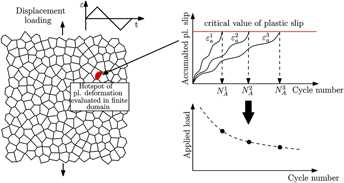
The material degradation is connected to plastic deformation via the rate of the accumulated plastic slip defined in Eq. (12), such that the accumulated plastic slip can be considered as the fatigue indicator parameter (FIP). Hence, a fatigue crack initiates, when a critical value of the accumulated plastic slip is reached, as detailed in the following. In this work, the algorithm to determine the fatigue crack initiation time is introduced (Fig. 1). To be able to estimate the crack initiation time, a crack-free material cyclically loaded with a given strain amplitude and R = −1 (cycling loading with the same amplitudes in tension and compression and an average stress of 0) is considered, which is shown in the left part of Fig. 1. The distribution of the fatigue indicator parameter and its evolution is determined for a given strain amplitude
 $\varepsilon _{\rm{a}}^1$
.
Schematic sketch of the algorithm to estimate the fatigue crack initiation lifetime.

Similar to Manonokul and Dunne, Reference Manonukul and Dunne41 in this work, a material specific critical value of accumulated plastic slip is defined. If this value is reached, fatigue crack initiation takes place. Figure 1 shows on the left a material RVE and an identified hotspot of plastic deformation in the material. The evolution of this hotspot i.e., the evolution of accumulated plastic slip is shown exemplary in Fig. 1 for the three different strain amplitudes. During cyclic loading, the accumulated plastic slip increases monotonically, while the amount of plastic deformation might be unchanged in the initial stages of loading and unloading, which leads to plateaus. If the accumulated plastic slip reaches the critical value, which is shown as a red line in the top right diagram of Fig. 1, the subsequent cycle number to fatigue crack initiation is reached. Thus, for any applied load, the evolution of accumulated slip can be triggered and an associated crack initiation cycle can be determined. This is visualized in the bottom right diagram of Fig. 1 and is termed Wöhler diagram for fatigue crack initiation. To be mesh independent, we used a gradient regularization of the damage model as described in Ref. Reference Boeff, Gutknecht, Engels, Ma and Hartmaier42.
To render the numerical values at integration points mesh independent and to introduce a damage length scale to the model, integration point values are averaged within a finite sphere. For each integration point, the sphere-neighborhood is determined in a postprocessing step. Furthermore, a finite element is considered to be completely damaged if the critical value of accumulated plastic slip is reached within the sphere around this element. Reference Boeff28
After an initial period, the plastic accumulated slip exhibits a constant rate and can be written as
 $${p^{{\rm{acc}}}} = \int {\dot{p}{\rm{d}}t} = {p^{\left( 0 \right)}} + N \cdot \Delta {p^{{\rm{sat}}}}\quad ,$$
where p (0) is the accumulated plastic slip in the initial unstable regime and Δp sat the amplitude of plastic slip in the stable regime. Following Castelluccio, Reference Castelluccio21 3–10 cycles are enough to reach the stable regime, while Manonokul and Dunne state that the saturated plastic slip per cycle is generally reached in less than 2 cycles. Reference Manonukul and Dunne41 Sharaf found that the saturation regime appears after 2–3 loading cycles. Reference Sharaf22 In this work, we used 2 cycles and assume that the saturation regime is reached. It is pointed out here, that a saturation in the plastic slip per cycle will only be reached if a material model with a monotonous hardening behavior is applied, whereas in the case of cyclic softening such a saturation cannot be expected.
With the critical accumulated plastic slip (p crit) as indicator for fatigue crack initiation, the critical number of cycles N crit to initiate a microcrack is given by
 $${N^{{\rm{crit}}}} = {{{p^{{\rm{crit}}}}} \over {\Delta {p^{{\rm{sat}}}}}}\quad .$$
In this case, Δp sat represents the amplitude of plastic slip in the stable regime. With this procedure, the number of cycles for crack initiation is determined, which allows us to plot S–N diagrams for fatigue crack initiation, as shown in Fig. 1. With the help of our model, we can study fatigue lifetime as a function of the microstructure morphology, hardening state, and defect distributions. Applying a series of different strain amplitudes, the individual cycle number to fatigue crack initiation can be plotted over the strain amplitude to result in a fatigue crack initiation diagram (see Fig. 7). In the present work, Eq. (17) represents a criterion for the very first stage of crack initiation (the so-called crack nucleation or incubation). The later stages of crack initiation, i.e., growth of microstructurally and physically small cracks, can in principle also be studied with the methods introduced here and will be the subject of forthcoming work.
III. NUMERICAL MODELING OF CYCLIC DEFORMATION
In this section, the micromechanical model described above is applied to study the deformation and damage mechanisms occurring during the cyclic deformation of a polycrystal. Special emphasis is put on characterizing the influence of different hardening mechanisms on the crack initiation time.
A. Localization of strain
For this study, 2D RVEs are generated using the dynamic microstructure generator (DMG) method Reference Tanaka and Mura27 as described above. The numerical simulations using 3D RVEs are computationally very costly. Thus, for the sake of numerical efficiency, in the present work, we only considered 2D simulations, which already provide important insights on the mechanisms of fatigue crack initiation and their relation to the microstructure.
The microstructural parameters taken into consideration for construction of the RVEs are grain size distribution, mean grain size, and standard deviation. The orientations of the grains (Euler angles) are selected randomly. The produced microstructure mimics a polycrystal with 360 equiaxed grains of BCC crystal with an average size of 60 μm, standard deviation of 5 μm and random orientations. To finish the RVE for micromechanical simulations, each grain is meshed with 4 node reduced integration type of elements. For each grain, approximately 80 elements under plane strain conditions are generated using Cubit. 43 It must be noted that the generated RVE from DMG is periodic and to apply the periodic boundary conditions, opposite surfaces must have exactly the same surface mesh, which requires a well-controlled meshing process.
In this section, the distribution of accumulated plastic slip within a polycrystalline microstructure and its evolution during cyclic deformation is investigated. Therefore, the RVE is cyclically loaded with a strain amplitude of εa = 0.25% and R = −1. For the numerical simulations, the material parameters for BCC ferrite steel are considered partly stemming from Inal et al. Reference Inal, Lebrun and Belassel44 and Mahmoody. Reference Mahmoody45 For the kinematic hardening parameters, no detailed parameters are found in literature for ferrite. In this work, the parameters A 1 and A 2 are loosely approximated inspired by work of Sharaf. Reference Sharaf22 The chosen material parameters are summarized in Table I and clustered into five sub-blocks according to their physical meaning. The elastic material behavior is orthotropic and thus can be described by elastic constants C 11, C 12, C 44. In the current work, we only consider {110}<111> slip systems for BCC.
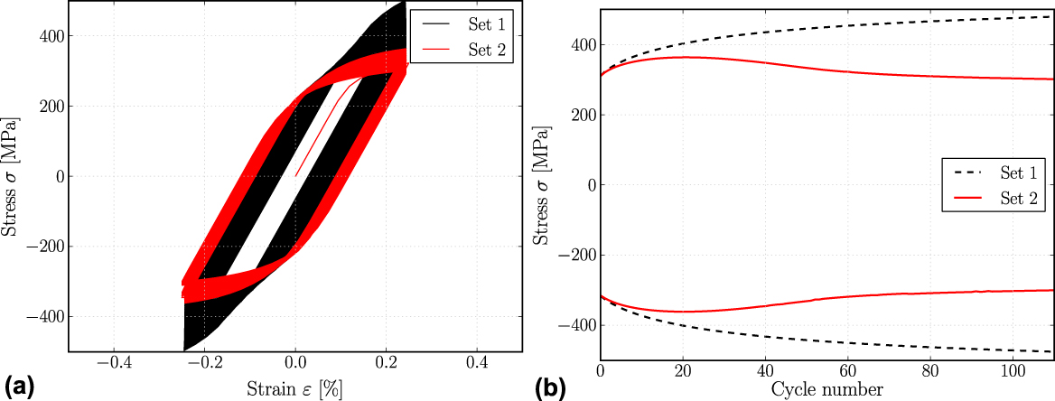
The material parameters specified in Table I are primarily used, while the influence of channel/wall-(cw)-evolution parameters is studied, so that two sets of material parameters are generated. These two sets of material parameters are applied to the same model. Within the first set, only isotropic and kinematic hardening are considered, while in the second set cw-evolution is considered additionally with the parameters as specified in Table I. The global stress–strain diagrams, homogenized over the entire RVE for the two sets of material parameters, are compared in Fig. 2.
Visualisation of global stress–strain hysteresis for the RVE is shown in figure (a) while the evolution of maximum and minimum stress amplitude is shown in figure (b).

Starting with the same microstructure configuration, the models differ in their cyclic behavior due to the cw-evolution. This effect is seen more clearly in the evolution of stress maxima and minima as a function of cycle numbers [Fig. 2(b)]. Set 1 (only isotropic and kinematic hardening, no cw-evolution) reveals a monotonous increase of maximum stress during cycling loading with a constant total strain amplitude. Hence, the local plastic slip per cycle is rather constant, giving rise to an increase in stress due to isotropic hardening, and this saturation in local plastic slip is reached within a small number of cycles [Fig. 4(a)]. In contrast, the stress maxima of set 2 (isotropic and kinematic hardening and cw-evolution) increases during the first cycles, but in cycle 20 cyclic softening sets in. This leads to a difference of approximately 150 MPa in the stress levels of set 1 and set 2 after 110 cycles of loading.
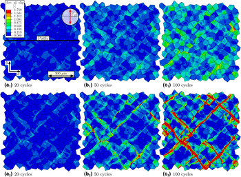
To analyze local deformations in the RVE, the accumulated plastic slip after 20, 50 and 100 cycles is visualized in Figs. 3(a1)–3(c1) for set 1 and Figs. 3(a2)–3(c2) for set 2. Comparing both sets individually from left to right, the distributions for both sets of material parameters have in common that the mean value of accumulated plastic slip increases with increasing cycle number. This is indicated by a growing number of grains with higher levels of plastic slip. The plastic slip distribution of set 1 is rather homogeneous. Plastic deformation starts in grains with a high Schmid factor [Fig. 3(a1)]. During cyclic deformation, these grains further accumulate plastic strain but the distribution within these active grains is rather homogeneous [Fig. 3(c1)]. In set 2 the plastic deformation is starting from nearly the same situation of accumulated plastic slip after 20 cycles [compare Figs. 3(a1)–3(a2)]. However, due to the cyclic softening starting in cycle 20, plastic slip starts to localize in specific regions for set 2 [Fig. 3(a2)]. During further fatigue loading these plastic regions localize even more and the accumulated plastic slip distributes in a band like structure within the RVE [Fig. 3(c2)].
The accumulated plastic slip distribution of set 1 is given in (a1–c1), while the accumulated plastic slip distribution of set 2 is given in (a2–c2) for 20, 50, and 100 cycles, respectively. The strain amplitude is εa = 0.25%.

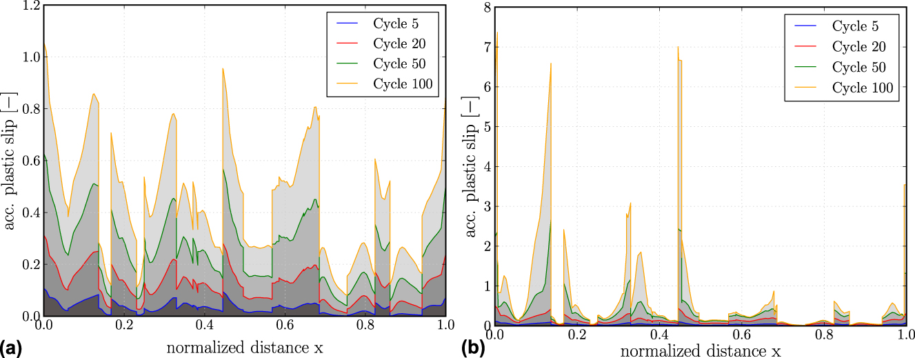
For further investigation of the accumulated plastic slip distribution, a path plot through the RVE is analyzed. The position of the path plot is defined in Fig. 3(a1). The path plots for the accumulated plastic slip for set 1 and set 2 after different numbers of loading cycles are given in Fig. 4. The evolution of accumulated plastic slip of set 1 exhibits minima and maxima that are occurring at the same positions. Also, the shapes of the distributions at different time steps are nearly identical, while only the amount of accumulated plastic slip increases. Hence, it is concluded that the plastic slip along the path scales proportionally to the number of cycles for the parameter set 1. This indicates that the local plastic slip per cycle has saturated after a small number of cycles. In contrast to this, the distributions for the material parameter set 2 show a strong localisation in sharp maxima. These maxima are distributed at similar locations as for parameter set 1. However, due to the softening behavior observed for the parameter set 2 after 20 cycles, the local plastic slip per cycle keeps increasing for some regions along the path, giving rise to some very sharp peaks in which extremely high values of plastic slip are reached. In many other regions, the plastic slip remains rather unchanged or increases only at a comparably lower rate.
Visualisation of the accumulated plastic slip along the path defined in Fig. 3(a1) after 5, 20, 50, 100 loading cycles for the model using the material parameter set 1 in (a) and for the parameter set 2 in (b). Note that the y-axis showing the accumulated plastic slip has a different scale.

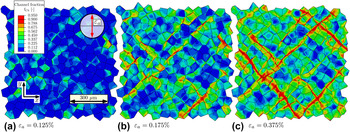
The strong localization of the accumulated plastic slip in band-like structures is caused by the cyclic softening originating in the model for channel and wall evolution, which describes a cyclic softening as seen in Fig. 2(b). The parts of the RVE, where most plastic strain occurs, become softer such that the accumulation proceeds faster in a self-amplifying way. Figure 5 shows the distribution of the channel volume fraction f Ch for three different strain amplitudes. No channel volume fraction, visible as blue regions, indicates areas in the microstructure showing no dislocation structuring, while regions indicated by red reveals regions where dislocation substructure has formed and the channel volume fraction is higher than 90%. For the three strain amplitudes εa = 0.125%, εa = 0.175% and εa = 0.375%, the distributions are plotted after 200, 116 and 22 cycles representing situation where the channel volume fraction f Ch reached 95% locally in the microstructure for the first time. Starting with the smallest strain amplitude visible in Fig. 5, the distribution of channel volume fraction is shown. Several grains show a channel fraction of 50% but the majority of grains show no significant dislocation structuring. Increasing the strain amplitude to 0.175%, the channel fraction distributes more homogeneously throughout the microstructure, visible by the majority of the grains showing a volume fraction of channels around 50%. Only some regions show strong plastic activity spreading over several grains, which indicates a high volume fraction of channels in specific regions. These channel bands increase in size for the strain amplitude of 0.375% and spread throughout the whole RVE. Note that the channel volume fraction is closely coupled to the accumulated plastic slip and shows a similar distribution, which can be seen comparing Figs. 5(b) and 5(c) with Fig. 3(c2). Note however, the difference in strain amplitude between those figures.
Visualisation of the channel fraction for three different strain amplitudes as given in the legends. For the three strain amplitudes, the situation is plotted when the volume fraction reached f Ch = 0.95 locally for the first time. Subfigure (a) shows the distribution for εa = 0.125% after 200 cycles, subfigure (b) for εa = 0.175% for 116 cycles and subfigure (c) for εa = 0.375% after 22 cycles.

B. Crack initiation time
In the following, a systematic study on the accumulation of plastic strains and the resulting crack initiation time is performed. To accomplish this, the scheme introduced in the earlier section is used, which enables us to estimate the fatigue crack initiation time based on the chosen fatigue indicator parameter. The fatigue crack initiation time is analyzed for an RVE consisting of 360 equiaxed grains with a rather homogeneous grain size distribution and a mean grain size of 60 μm and a standard deviation of 5 μm. A series of strain amplitudes ranging from εa = 0.05% to εa = 0.75% is applied and the accumulation of plastic strains is investigated. Each grain is meshed with approximately 80 reduced integration elements under plane strain conditions.
As crack initiation time is known to depend strongly on the underlying microstructure, a significant scatter in simulation results is expected to appear. Therefore, a number of similar RVEs are constructed, which share the same statistical properties e.g., mean grain size, grain size distribution. The approach to determine fatigue crack initiation is applied to the group of RVEs to obtain statistically reliable results. Similar to Reference Castelluccio21,Reference Sharaf22,Reference Evrard, Aubin, Degallaix and Kondo40 a small number of loading cycles per load amplitude is applied. The accumulated plastic slip for the stabilized cycle is determined and extrapolated to estimate the cycle number to fatigue crack initiation. Since our estimation of the lifetime according to Eq. (17) depends on a saturated value for the local plastic slip, only the parameter set 1 (Table I) is applied here, i.e., evolution of channels and walls is disregarded. For parameter set 2 and in particular if cyclic softening occurs, a saturation of local plastic slip might occur only after a large number of cycles, or in fact, not at all.
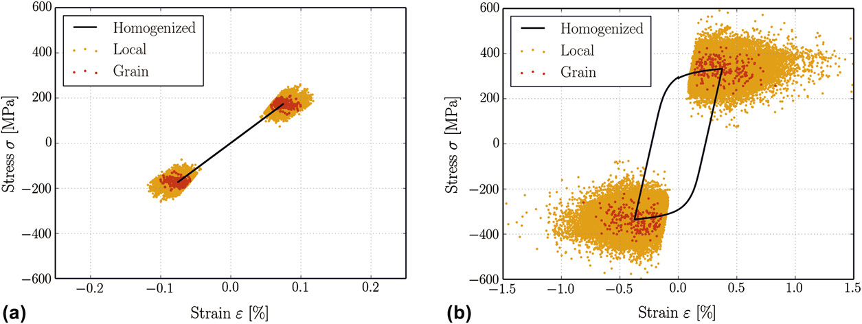
The stabilized stress–strain hysteresis for two different applied strain ranges is shown in Fig. 6. The global stress–strain response of the RVE is plotted as black solid line, while the stress–strain values, i.e., σ22 and ε22 of each individual integration point are plotted (orange) at the maximum and the minimum applied strain of a cycle, to visualize the heterogeneity of local deformations. Additionally, the grain averaged stress and strain state is plotted in thick (red) points. Whereas the stress–strain hysteresis of Fig. 6(a) has no measurable width, for the hysteresis of Fig. 6(b) a significant plastic strain range is visible.
Saturated global stress–strain cycle (a) εa = 0.075% (b) εa = 0.375%. The local values (thin orange points) and the complete grain averaged values (thick red points) are plotted at the maximum and the minimum applied strain level.

The plotted strain range of the diagrams is chosen to be four times the applied strain range to make the local deformations for the two graphs comparable. For the first applied strain range, the local deformations are rather homogeneous varying for the maximum applied strain marked with red points from 0.05% to 0.11%. The stresses vary from 110 to 210 MPa. From the comparison of the local deformations of Figs. 6(a) with 6(b) it is obvious that the scatter in local deformation increases with increasing strain amplitude. While the increase in scatter of the local stresses is approximately 250 MPa (a factor of 2.5) for a strain amplitude of εa = 0.375%, the scatter in strains increased to 1.4%. This is a factor of 28 compared to the strain amplitude of εa = 0.075% in Fig. 6(a). Hence, the deformation heterogeneity increases with increasing strain amplitude, while a pronounced increase is observed for the strain range of local deformation.
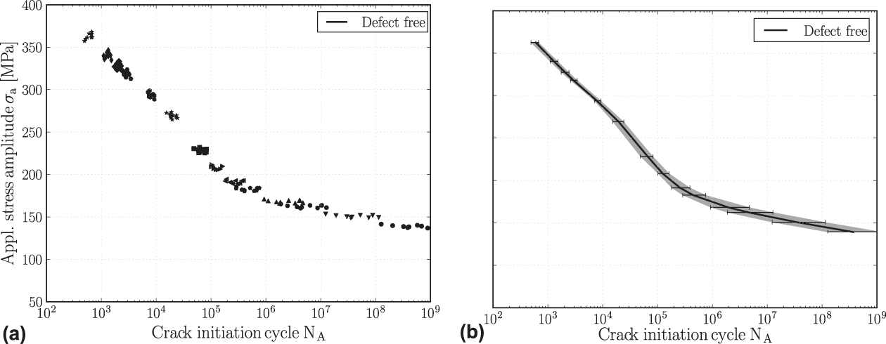
Using the crack initiation method introduced earlier, the S–N diagram for the defect free material is plotted. As a material constant for the determination of the crack initiation period, a critical accumulated slip of 300 (refer to Eq. 17) is chosen exemplary. Reference Manonukul and Dunne41 This value needs to be fitted to the material analyzed through the experimental data. Figure 7(a) shows the raw data for 10 different RVEs subjected to the same load sequence, while every single point is the result of one simulation with a constant applied strain range. The results for one strain amplitude are marked with the same symbol type. Each individual point in the diagram corresponds to an individual RVE and a certain applied strain amplitude leading to 10 points per strain amplitude. As the simulations are strain controlled, a slight scatter in the global stress amplitude appears, which corresponds to the scatter in y-direction, while the scatter in x-direction is due to microstructural influences. The effective properties in the form of mean values and maximum deviation, defined as difference between maximum and minimum value for the crack initiation cycle, are given in Fig. 7(b). The determined maximum and minimum deviations are marked, while the band of possible results is shown in gray.
Visualisation of fatigue crack initiation diagram with applied stress amplitude plotted over determined crack initiation cycle. Figure (a) shows the raw data for 10 different RVEs, while figure (b) shows the mean value with a band of maximum deviation. Note that the simulations are strain controlled, such that there is a small variation in the homogenised stress amplitudes in figure (a).

It can be observed that the band width increases with decreasing strain range. This is due to the transition of plastic deformation behavior within the RVE. While the plastic deformations for higher strain amplitudes spread throughout the whole RVE and are influenced by nearly the whole microstructure, for smaller strain amplitudes, the plastic deformations are very local and depend on individual grains. In the diagram, three different regions can be identified. For lifetimes below 104, a linear decreasing region can be found. This region is characterized by plastic deformation, which takes place in the whole RVE and is rather homogeneous. For crack initiation numbers higher than 5 × 10⁵, a region with a smaller decay can be found. This regime is characterised by very localized plastic deformations at specific hot spots or within individual grains with a high Schmid factor. This deformation is very heterogeneous. In between these two regimes, a transition regime is observed in which the very homogeneous plastic deformation transforms to a rather heterogeneous deformation with decreasing strain amplitude. Analysing the statistical scatter which is plotted as gray region in Fig. 7(b), it is apparent that the width of the gray band increases with decreasing strain amplitude. This means that the difference in predicted lifetime within the considered RVEs has a higher scatter for lower strain amplitudes.
IV. CONCLUSIONS
In this work, a micromechanical model for fatigue of polycrystalline materials is proposed and applied to study the influence of cyclic hardening and softening on the localization of plastic strain and the initiation of a fatigue crack. To achieve this, a crystal plasticity constitutive model has been used to predict the influence of microstructure and constitutive modeling of cyclic work hardening on the accumulation of plastic slip in different regions of the microstructure. The microstructure was created in the form of RVEs of polycrystalline material with equiaxed grains and a random texture. It is observed that the results of the micromechanical model describe crack initiation life during fatigue exhibit several features that are also observed in experiment, e.g., the shape of the S–N curves or the fact that cyclic softening leads to a pronounced plastic slip localization in slip bands. The results have shown the capabilities of this model to predict crack initiation life in polycrystalline materials such that, in future applications, it can be used to investigate the mechanisms of fatigue crack initiation and how they depend on microstructure and constitutive material behavior.