


1. MOTIVATION AND RESULTS
Consider a decision maker who must assign subjects to one of several treatments. The success of treatments is measured by some outcome variable Y, and the decision maker is an expected value maximizer, so if she knew the expected outcomes induced by different treatments, her problem would be trivial. However, her information is incomplete; specifically, she only knows that one of a set

of states of the world, identified with mappings from treatments to expected outcomes, has obtained. Because no probability distribution over

is provided, she faces a decision problem under ambiguity (or “Knightian uncertainty”).
Manski (in press; see also Brock, 2004) recently analyzed the special case of this problem that arises when the ambiguity is due to missing data, proposing minimax regret as the decision criterion and analyzing some of its features. This note extends his analysis by considering a more general decision environment and, more importantly, by allowing for finitely many as opposed to two treatments. The binary problem's most intriguing feature, namely, that the minimax regret treatment rule assigns positive fractions of the population to either treatment unless one of the treatments is dominant, turns out not to generalize.
It is helpful to first restate the problem analyzed by Manski. Let there be treatments t = 1,…,T that induce (random) potential outcomes (Yt)t=1T over a bounded support, say, Yt ∈ [0,1]. If μt ≡ E(Yt) were known for every t, treatment would be assigned accordingly. But observations of Yt are plagued by missing data, and only a fraction pt of realizations is observed. Defining E1(Yt) ≡ E(Yt|Yt is observable) and E0(Yt) ≡ E(Yt|Yt is missing), the decision maker's knowledge of μt is summarized by

where E1(Yt) and pt are known but E0(Yt) is not. (I will abstract from estimation problems; thus “observable” is synonymous with “known.”) It follows that μt ∈ [pt E1(Yt),pt E1(Yt) + 1 − pt], but this information may not suffice to identify the best treatment; nonetheless, some treatment rule has to be adopted. Manski (in press) proposes to evaluate treatment rules according to minimax regret. To formalize this, denote treatment rules by δ ∈ ΔT−1, where ΔT−1 is the (T − 1)-dimensional unit simplex in

and the tth component of δ, δt henceforth, is the probability assigned to treatment t. Also letting

collect all possible configurations of (μt)t=1T, the minimax regret ranking is given by

Because [sum ]t δt μt is the expected outcome induced by treatment rule δ, this can be thought of as a maximin criterion but with respect to ex-post efficiency loss rather than utility. For motivations and further discussions, see Manski (2004) and Stoye (2005b); the latter also contains many historical references. Manski (in press) finds the minimax regret treatment rule when T = 2. A salient observation, replicated in Brock (2004) and as Corollary 1 in the discussion that follows, is that unless the better treatment is identified from the data, this treatment rule is mixed; i.e., it allocates a positive fraction of the population to each treatment.
I generalize this result in two ways. First, I provide the solution for arbitrary finite T. Second, I allow for different informational settings as captured by information sets

. Specifically, the only structure imposed on

is that if

and

, then

contains all of the states {st}t=1T, where st ≡ (μ1,μ2,…, μt−1,μt,μt+1,…, μT). Intuitively, this amounts to two restrictions:
- The bounds that one is able to place on μt are tight; i.e., they are achieved in some feasible state of the world s.
- Cross-restrictions between states are limited; in particular, it is possible that some treatment t is as good as possible, and all other treatments are as bad as possible, at the same time.
The Manski (in press) scenario emerges as special case with

as given before, but the requirement that

is significantly weaker. Bounds on expectations can arise from many other sources of partial identification as surveyed in Manski (2003), interval data and bounds on cumulative distribution functions being but two examples. Similar informational settings also occur in the literature on interval probabilities (Walley, 1991) and in robust Bayesian inference (Wasserman and Kadane, 1992). As long as there are no or appropriately limited cross-restrictions, the present analysis will apply to all of these cases.
The according generalization of Proposition 1 in Manski (in press) is stated next. It is established by analyzing a fictitious zero-sum game between the decision maker and a malicious Nature whose expected utility equals the decision maker's expected regret. The Nash equilibria of this game are known to characterize all minimax regret treatment rules. In a first step, I show that Nature's action set can be reduced to {st}t=1T (hence the requirement that

contain this set). It is then possible to analytically characterize the equilibria. A complication arises because there are two mutually exclusive types of them, captured subsequently by cases (i) and (ii) in Proposition 1 with treatment rules δ respectively δ*. (At their boundary in parameter space, a hybrid case obtains and is labeled (iii).) In either equilibrium, the expected utility of action st to Nature turns out to be indexed by a weighted average λt ≡ δt μt + (1 − δt)μt of the according treatment's best and worst case expected outcome, the weight being the probability with which the treatment is assigned. With this in mind, the expressions for δ respectively δ* can be derived from Nature's best response condition.
PROPOSITION 1. Order treatments such that μ1 ≥ ··· ≥ μT, where the tie-breaking rule is arbitrary. Let ν ≡ maxt{μt}, call a treatment t maximin if μt = ν, and define δ ∈ ΔT−1 and

implicitly by

and t* ∈ {1,…,T} by
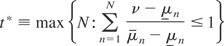
with the convention that

. Consider the following cases.
(i) If t* > max{t : δt > 0}, then δ* = δ is the unique minimax regret treatment rule.
(ii) If t* ≤ max{t : δt > 0} and

, then δ* ∈ ΔT−1 is a minimax regret treatment rule iff

(iii) Otherwise, δ* ∈ ΔT−1 is a minimax regret treatment rule iff

for some λ* ∈ [max{λ,μt*+1},μt*].
A sufficient condition for the minimax regret treatment rule to be unique is that the maximin treatment is unique and

.
COROLLARY 1. Let T = 2; then the unique minimax regret treatment rule is

2. PROOFS AND DISCUSSION
Proof of Proposition 1. Consider the following zero-sum game between the decision maker and Nature: (i) The decision maker chooses a treatment rule δ ∈ ΔT−1. Nature chooses a potentially mixed strategy

, i.e., a distribution over states of the world. (ii) A neutral metaplayer draws

according to σ. (iii) The decision maker's loss is R(δ,s) ≡ maxt{μt} − [sum ]t δt μt. Both players maximize expected utility. Then there exist convex sets

and

is a Nash equilibrium of the game

; furthermore,

is the set of minimax regret treatment rules (e.g., see Stoye, 2005a, App.).
Assume treatments are ordered as stated in the proposition. Fix any treatment rule δ. Any best response to δ is supported on

The objective function increases in μm iff μm = maxt{μt} and decreases in it otherwise (weakly so if δt = 0). Thus, Nature always has a best response in the set {st}t=1T as defined earlier. Consider the restricted game in which Nature's strategy space is reduced to this set; then it follows that any Nash equilibrium of this game is a Nash equilibrium of the unrestricted one. Because, furthermore, every minimax regret treatment rule δ* is a best response to every worst case prior σ*, an exact characterization of the minimax regret treatment rules for the restricted game implies an exact characterization for the unrestricted one. I will now provide the former.
In the restricted strategy space, Nature's strategy σ can be identified with a vector σ ∈ ΔT−1, where σt = Pr(s = st). Observe that given σ, treatment t has expected outcome μt = (σt μt + (1 − σt)μt).
Let (δ*,σ*) be a Nash equilibrium. To be a best response to σ*, δ* must solve

The left-hand expectation does not vary with δ, so that δ* must maximize Es|σ*(Σtδt μt), i.e., expected outcome given σ*. Hence, δt* > 0 only if σt* μt + (1 − σt*)μt = μ* ≡ maxt{σt* μt + (1 − σt*)μt}. Furthermore, (δ*,σ*) is known to induce expected outcome μ*; observe in particular that μ* ≥ ν.
If σ* maximizes regret against δ*, it must also maximize regret against δ* under the additional constraint that σt* μt + (1 − σt*)μt ≤ μ*,∀t, because by construction, this constraint will not bind at σ*. Hence, σ* must solve
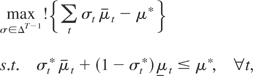
where I also use the knowledge that in equilibrium, Es|σ*([sum ]t δt μt) = μ*.
The preceding problem is linear in every μt; because treatments are ordered according to μt, it is solved by maximizing the probability mass placed on lower numbered treatments:

where

.
But σ* being a best response to δ* also requires that

and

Hence, δ* is partially characterized by the fact that there exists λ s.t.

Of course, δt* must also be nonnegative, so that (μt − λ*)/(μt − μt) can be replaced with max{[(μt − λ*)/(μt − μt)],0} in (2). To proceed with the characterization, one must distinguish two cases.
Case 1. For all t, δt* = max{[(μt − λ*)/(μt − μt)],0}. Because also Σtδt* = 1, this case generates (T + 1) linear equations in (T + 1) unknowns. If one guesses λ* = maxt{μt}, then it is easily seen that Σtδt* = 0 is implied. On the other hand, a guess of λ* = μ1 implies that δ1* = 1 and hence Σtδt* ≥ 1. For intermediate values of λ*, the implied value of Σtδt* is continuously decreasing in λ*; hence Σtδt* = 1 holds for exactly one λ. The case therefore generates a unique candidate δ*.
Best response conditions now constrain σ* as follows:

If t* > max{t : δt > 0}, then the preceding constraints are consistent with (1). It can then be straightforwardly verified that (δ*,σ*) constitutes a Nash equilibrium and that δ* is characterized as in case (i) in Proposition 1. If t* ≤ max{t : δt > 0} and the preceding constraints imply that Σtσt* > 1, the equilibrium fails. If Σtσt* ≥ 1 is implied, the equilibrium will exist but may be nested within case (iii).
Case 2. For some t, δt* > max{[(μt − λ)/(μt − μt)],0}. This implies that the decision maker chooses with positive probability some treatments t′,t′′,… with σt′* = σt′′* = ··· = 0; hence their expected outcomes are equal to μt′,μt′′… This is consistent with δ* being a best response only if μt′ = μt′′ = ··· = μ*; because μ* ≥ ν, it must be the case that all of these treatments are maximin and that μ* = ν.
Expression (1) now fully characterizes σ*. If

, then

This is consistent with (2) only if μt* = λ*. With λ* thus defined, expression (2) bounds every δt* from below. If these lower bounds sum to more than one, the candidate equilibrium fails. Otherwise, every δ* that fulfills the bounds and has Σtδt* = 1 is a best response to σ*. (If there is exactly one maximin treatment, δ* is unique.)
In the knife-edge case that

, λ* may not be uniquely determined. However, inspection of (2) reveals that λ* ≤ μt* (because δt** ≥ 0) and that λ* ≥ μt*+1 (because δt*+1* = 0). An alternative lower bound on λ* is generated by assuming that all inequalities in (2) bind, i.e., by presuming case (i) in Proposition 1. (If this constraint binds, both cases yield valid equilibria, with the set of minimax regret rules characterized under case 2 containing the δ* characterized in case 1.) Any choice of λ* that is consistent with these constraints will generate a δ* s.t. (δ*,σ*) constitutes a Nash equilibrium.
That one of the cases will yield a Nash equilibrium is not obvious from the preceding discussion. Note, however, that the cases are exhaustive, and by existence of a Nash equilibrium, one of them must yield at least one equilibrium. If both cases yielded valid sets of equilibria with the equilibrium from case (i) not contained in the equilibria from case (ii), the set of Nash equilibria would be disconnected, contradicting convexity. Also, sufficiency of the conditions is easily established. █
Proof of Corollary 1. Let T = 2 and μ1 < μ2 and also μ2 < μ1. (For the other cases, δ* is obvious.) Assume by contradiction that μ* = ν; then σt* will be zero if t is maximin and will be less than one otherwise, implying that Σtσt* < 1. Hence, case (i) in Proposition 1 applies, and (2) can be solved for δ*. █
Mathematically, Proposition 1 implies that the set of minimax regret treatment rules is the convex hull of a finite number of extremal treatment rules. Although somewhat tedious to describe, these extrema are easy to evaluate, and once identified, their validity can be checked by paper-and-pencil methods.1
MATLAB code that evaluates Proposition 1 is posted on the author's Web page at http://homepages.nyu.edu/∼js3909/.
Examples of either form of nonunique solutions are given in an online appendix on the Web page mentioned in note 1.
Other than this, general intuitions about δ* seem to be limited to the fact that it is always supported on the t* best treatments in terms of the max max-ordering, i.e., according to μt, where t* is some number between 1 and T. Two more features are illustrated by the following examples.
Example 1
Let T = 2 and let bounds on μt be as follows:

Then

uniquely.
Example 2
Let T = 3 and let bounds on μt be as follows:

Then δ* = (1,0,0) uniquely.
First, Example 2 is generated from Example 1 by adding a treatment that is seemingly like treatment 2.3
The result depends, however, on the presumption that treatments 2 and 3 are not actually the same, because the possibility of their outcomes being different is crucial.
Second, δ* in Example 2 is not mixed; i.e., the most salient aspect of the two-treatment case does not carry over. This finding is of general interest because researchers investigating minimax regret decision rules usually find these to mix, often in contrast to maximin utility rules (Bergemann and Schlag, 2005; Brock, 2004; Manski, 2004; Schlag, 2003; Stoye, 2005a). To understand why it obtains, it is instructive to informally prove that δ* will always mix in the case of two (nondominating) treatments. Suppose by contradiction that δ* is concentrated at t = 1; then Nature's best response in the fictitious game is to deterministically choose state s2. But the decision maker's best response to that would be to assign all subjects to treatment 2. The best response correspondence therefore cycles over pure strategies. In short, the result obtains because 2 × 2 anticoordination games have only fully mixed equilibria.4
In Example 1, the equilibrium is completed by setting

.
But this observation does not generalize to more complex games. In Example 2, one of Nature's best responses to δ* is to mix equally over s2 and s3; δ* then remains the decision maker's strict best response and hence is the unique minimax regret treatment rule. Notice that μ2 = μ3 is necessary for this to work; thus a nonmixing δ* obtains only in specific, although interesting, cases.


