





1 Introduction
To measure and retrieve complete electric-field information of ultrashort laser pulses is critical for optimizing or manipulating the ultrafast light field. As a popular method, like frequency resolved optical gating (FROG), spectral phase interferometry for direct electric-field reconstruction (SPIDER) can measure both the amplitude and phase of an ultrafast light field. Compared with FROG, SPIDER can support real-time operation at a much higher frame rate by directly reconstructing the spectral phase from one-dimensional spectrograms via only a two-step Fourier transform (FT) algorithm. However, the temporal filter in the process of the reconstruction degrades its fidelity and ability for the ultrashort laser pulse with complicated temporal/spectral structures or with a narrower spectral bandwidth. To avoid the disadvantage, some efforts have been reported to improve the spectral resolution and the measured signal-to-noise ratio (SNR), which include spectrum-space encoding[ Reference Wyatt, Walmsley, Stibenz and Steinmeyer 1 ], wavelet transform as a substitute for FT[ Reference Deng, Wu, Chen, Chai, Wang and Zhang 2 ], two-dimensional spectral shearing interferometry[ Reference Birge, Ell and Kärtner 3 ], and so on. By combining spectral phase interferometry with two-step phase-shifting (TSPS), we have successfully reformed SPIDER (TSPS-SPIDER)[ Reference Zheng, Cai, Pan, Zeng, Li, Li, Zhu, Lin and Xu 4 ] to eliminate experimentally the direct current (DC) component of the recorded spectral interferograms, which results in not only the perfect selection of the alternating current (AC) component, but also the great promotion of the SNR of the AC information. Our experiments verified that TSPS-SPIDER has a higher measured SNR and fidelity, and a stronger ability for an ultrafast pulse with complicated temporal/spectral structures or with narrower spectral bandwidth by two measurements of spectral interferometry with the π-phase shift.
In the last decade, ultra-intense and ultrashort laser pulses have drawn considerable attention for many important applications in extreme-physics frontiers, including laser fast ignition, laser particle acceleration, laser-driven high-brightness radiation sources, quantum electrodynamics, etc.[ Reference Kodama, Norreys, Mima, Dangor, Evans, Fujita, Kitagawa, Krushelnick, Miyakoshi, Miyanaga, Norimatsu, Rose, Shozaki, Shigemori, Sunahara, Tampo, Tanaka, Toyama, Yamanaka and Zepf 5 – Reference Di Piazza, Müller, Hatsagortsyan and Keitel 9 ]. It is critically important to accurately characterize the pulses to manipulate the pulse duration, shape and contrast[ Reference Lin, Feng, Cai, Lu, Zeng, Wang, Xu, Li and Yuan 10 ], which seems to provide an important application scenario for TSPS-SPIDER. Unfortunately, this kind of laser pulse usually has a low repetition rate or only a single shot[ Reference Chu, Gan, Liang, Yu, Lu, Wang, Wang, Xu, Lu, Yin, Leng, Li and Xu 11 , Reference Sun, Long, Song, Shen, Liu, Zhao, Zhang, Yu, Peng and Leng 12 ].
In spite of the fact that TSPS makes great improvement based on traditional SPIDER[ Reference Cai, Chen, Zeng, Shangguan, Lu, Song, Ai, Xu and Li 13 ], TSPS-SPIDER needs two recordings for two spectral interferograms with the π-phase shift, thereby sacrificing its single-shot mode. Single-shot FROG[ Reference Yang, Rho, Seo and Kim 14 – Reference Diels and Rudolph 16 ] can reconstruct iteratively the ultrafast optical-field by two-dimensional phase-retrieval from the measured time–frequency trace[ Reference Kane and Trebino 17 , Reference O'Shea, Kimmel, Gu and Trebino 18 ]. However, its iterative algorithm limits its measurement fidelity, especially for pulses with fine temporal/spectral structures[ Reference Jolly, Lytova, Vallières, Légaré, MacLean and Fillion-Gourdeau 19 , Reference Cai, Chen, Zheng, Shangguan, Zeng, Lu, Wang and Xu 20 ]. Accordingly, high-quality single-shot measurement for complete construction of ultrafast light fields still faces challenges. This paper presents a single-shot TSPS-SPIDER. It avoids the disturbance from the DC components of the recorded spectral interferograms, but does not require an iterative algorithm. Accordingly, this work provides a powerful way to characterize the temporal/spectral structures of ultrafast laser pulses with high accuracy and high fidelity in a single-shot mode.
2 Principle and design of single-shot TSPS-SPIDER
A schematic diagram of our single-shot TSPS-SPIDER is shown in Figure 1, where the target laser pulse is split by a beam splitter (BS). After passing through a half-wave plate (HWP-1) for rotating the polarization, the transmission part is strongly chirped by a pulse stretcher (PS), which is then divided into two sub-beams (CP-1 and CP-2) by a non-polarization cube splitter (NPCS-1). Both the sub-beams are focused to a sum-frequency crystal (SFC, beta barium borate (β-BBO)). A time delay line (TDL-2) works to generate a relative delay time between the sub-beams. The reflected part is used as the target, which, after being delayed by another TDL (TDL-1), goes through the β-BBO crystal for nonlinear sum-frequency with the two sub-beams, separately. Consequently, two sum-frequency pulses (SFPs: SFP-1 and SFP-2) are generated with a relative delay time
$\tau$
 induced by the third TDL (TDL-3), which go forward to another NPCS (NPCS-2) by its two orthogonal incident surfaces to output two beams including parts of SFP-1 and SFP-2. Accordingly, by using two spectrometers (SPM-1 and SPM-2), the two spectral interferograms can be recorded. According to the arrangement above, SFP-1 and SFP-2, which are generated from the optical sum-frequency between the target pulse and the monochromatic components sheared from CP-1 and CP-2, can be expressed as follows[
Reference Lin, Cai and Xu
21
]:


Schematic diagram of our single-shot TSPS-SPIDER. HWP-1, HWP-2, half-wave plates; BS, 50:50 broadband beam splitter; PS, pulse stretcher; TDL-1–TDL-3, time delay lines; M, mirror; FO, focal optics; SFG, sum-frequency generator; NPCS-1, NPCS-2, non-polarization cube splitters; SIF-1, SIF-2, spectral interferograms; SPM-1, SPM-2, spectrometers.

Figure 1 Long description
The diagram illustrates an optical layout starting from a 25 f s 800 H z 800 n m Laser source. The beam travels left to a series of three mirrors M, then upward to a B S broadband beam splitter.
One path continues right through H W P 1, a pulse Stretcher, and N P C S 1. A second path is diverted down and right through M and T D L 1. A third path splits from N P C S 1 downward through T D L 2 and M.
These three beams converge at F O focal optics. The top beam C P 2 and bottom beam C P 1 flank a central Target beam. They meet at an S F G sum-frequency generator.
Post-S F G, two signal beams S F P 1 and S F P 2 pass through a Lens and reflect off a mirror M. The light passes through T D L 3 and enters a dashed box containing the detection assembly. Inside this box, the light hits N P C S 2, which splits the signal into two paths: S I F 1 leading to S P M 1 and S I F 2 leading to S P M 2. Rainbow-colored gradients represent the spectral pulses at various stages.
Correspondingly, the outputs from NPCS-2 can be described as

recorded by SPM-1 and

by SPM-2. Here, T and R are the reflection and transmission, respectively, of NPCS-2 with R + T = 1; τ and Ω are the relative delay time between the SFPs and the corresponding instantaneous frequency difference between the chirped pulse pair, respectively, while
$\theta \left(\omega \right)=\varphi \left(\omega \right)-\varphi \left(\omega -\Omega \right)$
 is the spectral phase difference. The first and second terms of Equations (3) and (4) correspond to the DC term, while the third term corresponds to the AC term of the interference spectrum. Obviously, SPM-1 captures the spectral interferogram (SIF-1) of the transmission part E
1t(ω) of E
1(ω) and the reflection E
2r(ω) of E
2(ω), while SPM-2 captures the spectral interferogram (SIF-2) of the reflection E
1r(ω) of E
1(ω) and the transmission E
2t(ω) of E
2(ω) from NPCS-2. Further, φ
1 and φ
2 are the appendant phase differences[
Reference Yu, Jiang, Zeng, Jing and Jiang
22
] between E
1t(ω) and E
2r(ω), E
1r(ω) and E
2t(ω), respectively.
According to the description above, the total incident power of NPCS-2 is |E 1(ω)|2+|E 2(ω)|2, which shall be equal to the sum of the powers of SIF-1 and SIF-2 if the energy loss in NPCS-2 can be ignored. By using Equations (3) and (4), we can obtain

Energy conservation requires that the above equation holds for all frequencies; thus

where m is an integer. Equation (6) means that, in this setup, a pair of spectral interferograms is recorded with a phase shift of π. Both φ 1 and φ 2 include the phases from the group delay dispersion (GDD) of NPCS-2. However, the GDD phases can be eliminated automatically by utilizing NPCS-2 with the balanced dispersions between its reflected and transmission beams.
From the two spectral interferograms with π-phase shift, as the TSPS-SPIDER[ Reference Zheng, Cai, Pan, Zeng, Li, Li, Zhu, Lin and Xu 4 ] did, we can directly remove the DC terms but double the AC terms with the spectral phase information, which can highly enhance the SNR and measuring accuracy.
3 Description of the experimental setup
Our experimental setup has been built according to Figure 1. The test pulses are from a commercial 800 Hz-25 fs-800 nm Ti:sapphire laser amplifier (Coherence Corporation, Legend Elite Duo HE+). Its output laser has an average power of 5.5 W and a bandwidth of Δλ = 50 nm or Δω = 2π × 23 Trad/s. The PS is a 60 mm × 70 mm ZF52 prism with its two corners cut for its 10-mm-wide entrance and exit, which is called a chamfer prism stretcher (CPS) here. This design allows the incident pulse to travel inside the prism by multiple rounds. When the pulse goes over a distance of 500 mm inside the CPS, it is chirped with a stretched pulse duration by Δτ
cp ≈ Δωβ
′′
d ≈ 15 ps[
Reference Iaconis and Walmsley
23
], where β
′′ is the group-velocity dispersion. Then, the chirped pulse is split into two beams (CP-1 and CP-2) by NPCS-2. TDL-1 consists of a pair of
$0{}^{\circ}$
 high-reflection mirrors and a pair of square-retroreflecting right-angle prism mirrors. The former is parallelly arranged to allow the incident pulse to go back and forth by five rounds as a compact optical-path folder, while the latter is adjustable for temporal synchronization with the chirp pulse.
The target pulse and the chirped pulse pair are focused together by a concave mirror (CM, f = 100 mm) into a 0.08-mm-thick
$\beta$
 -BBO crystal for nonlinear sum-frequency. Here, the target pulse polarizes horizontally, while the chirp beams are transformed into vertical polarization by HWP-1. The
$\beta$
 -BBO crystal is
$42.3{}^{\circ}$
 -cut for a type-II phase match to avoid self-second-harmonic backgrounds, thus improving the SNR. In order for a wider spectral bandwidth of sum-frequency[
Reference Iaconis and Walmsley
23
], the crystal is arranged so that the target pulse acts as an o-ray while the chirped pulses are e-rays. Correspondingly, the generated SFPs (SFP-1 and SFP-2) are centered at around 400 nm with a spectral shear
$\Omega$
 . Finally, the SFPs are combined by NPCS-2 to produce a pair of π-phase-shift spectral interferograms recorded by two same-version spectrometers (SPM-1 and SPM-2, Brolight Corporation, BIM-6601A15) with a sampling interval of 0.03 nm and a resolution of 0.08 nm. However, the unconformities of the recorded spectra, resulting from the response functions of the two spectrometers and the difference between the spectral transmission and reflection of NPCS-2 according to Equations (3) and (4), may lead to incomplete DC cancellation after subtracting the FTs of the interferograms, described as follows:

Equation (7) shows that the residual DC term originates from the nonuniform beam splittings of both NPCS-1 and NPCS-2.
During the measurement, we tune the spectral shear of SFP-1 and SFP-2 by adjusting the delay time between CP-1 and CP-2 with TDL2 and checking the central frequencies of SFP-1 and SFP-2. The interferograms are controlled by tuning the delay time τ of SFP-1 and SFP-2 with TDL3. Finally, in order to calibrate the spectral shear
$\Omega$
 , we can measure the spectral phase of a thickness-known glass and compare it with the corresponding theoretical calculation according to the Sellmeier coefficients[
Reference Ghosh
24
] to correct
$\Omega$
 .
In Figure 1, there is no additional dispersion to the test pulse, and it is thus a zero-additional-phase SPIDER (ZAP-SPIDER)[ Reference Baum, Lochbrunner and Riedle 25 ]. For comparison, we implement the measurements based on ZAP-SPIDER, two-step phase-shift SPIDER (CTP-SPIDER)[ Reference Cai, Chen, Zheng, Lin, Zeng, Li, Li and Xu 26 ] and SS-TSPS-SPIDER. SS-TSPS-SPIDER records two interferograms with both SPM-1 and SPM-2, whereas ZAP-SPIDER works with one of the interferograms from SPM-1 or SPM-2. CTP-SPIDER needs only one of the spectrometers, but has to get two π-phase-shifting interferograms by two measurements with HWP-2 rotated to shift its optical axis from horizontal to vertical orientation. Accordingly, all the measurements can be carried out without altering the existing system for effective comparisons.
4 Results and discussions
According to the description above, we firstly measured the spectral phase added to the same incident laser pulse by a 3-mm-thick BK7 glass with SS-TSPS-SPIDER, CTP-SPIDER and ZAP-SPIDER under the same parameters (
$\tau =0.9\;\mathrm{ps}$
 and
$\Omega =1.6\;\mathrm{THz}$
 ).
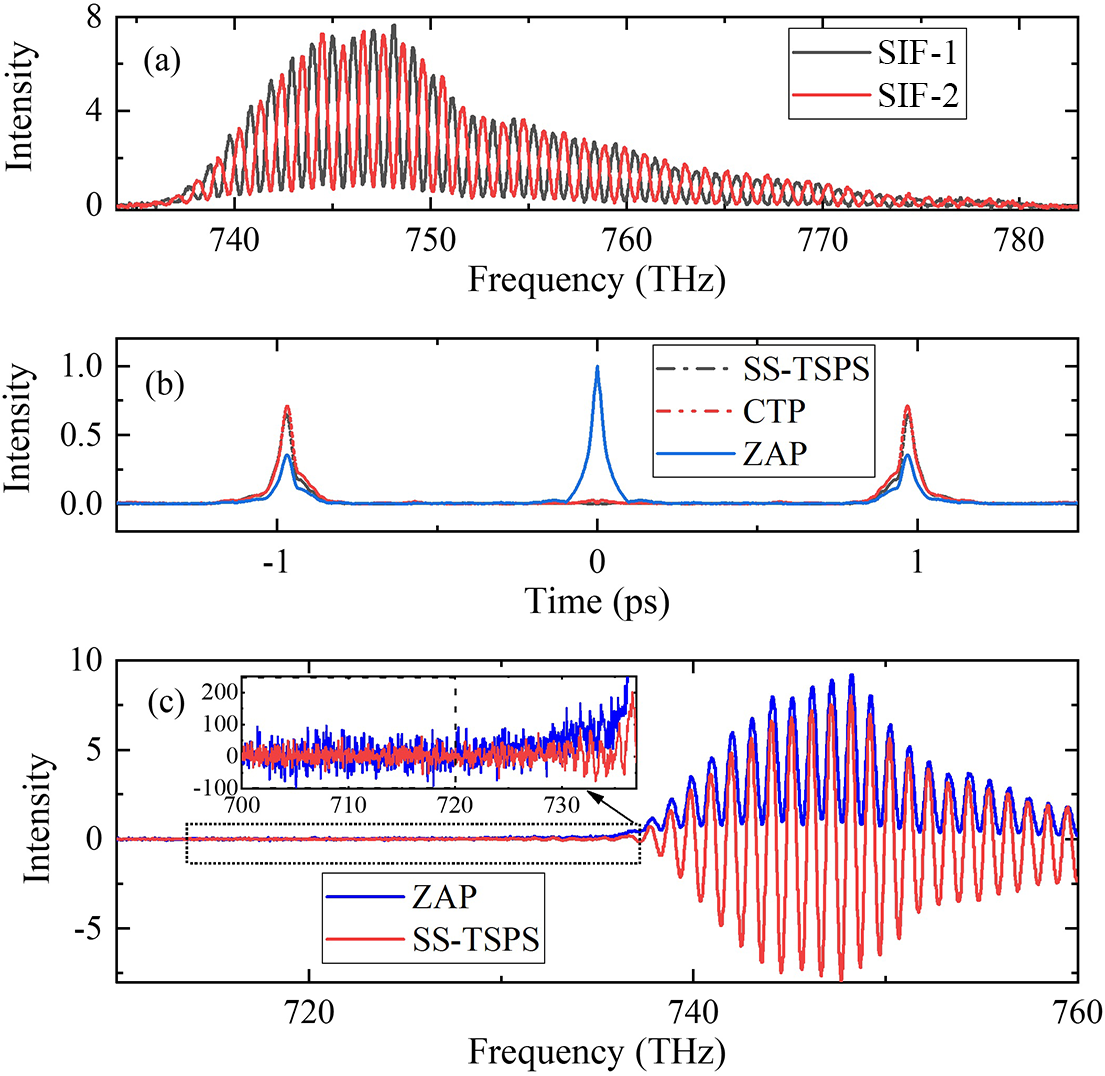
Figure 2(a) shows the spectral interferograms of SS-TSPS-SPIDER recorded with SPM-1 and SPM-2 under single-shot mode and marked by red and black lines, respectively. One can see that there exists obviously a π-phase shift between the two spectral interferograms as a theoretical prediction. One of the interferograms can be used as the result by ZAP-SPIDER. The two measurements of CTP-SPIDER were also made for two π-phase-shift spectral interferograms by using SPM-1 and HWP-2, which are highly consistent with those in Figure 2(a).
Measured results by SPIDERs: (a) spectral interferograms (SIF-1 and SIF-2) by SS-TSPS-SPIDER and ZAP-SPIDER, (b) their Fourier transform and (c) the measurement noise by the ZAP and SS-TSPS methods.

Figure 2 Long description
Panel a is a line graph with Frequency in T H z on the x-axis from 735 to 785 and Intensity on the y-axis from 0 to 8. It shows two highly oscillatory spectral interferograms, S I-1 in black and S I-2 in red, peaking near 748 T H z and tapering off toward higher frequencies.
Panel b is a line graph with Time in p s on the x-axis from -1.5 to 1.5 and Intensity on the y-axis from 0.0 to 1.0. Three traces are shown: S S-T S P S as a black dash-dot line, C T P as a red dotted line, and Z A P as a solid blue line. The Z A P trace shows a sharp central peak at 0 p s, while all three methods show smaller symmetric peaks near -1 p s and 1 p s.
Panel c is a line graph with Frequency in T H z on the x-axis from 710 to 760 and Intensity on the y-axis from -10 to 10. It compares Z A P in blue and S S-T S P S in red. Both show a high-amplitude oscillation starting around 738 T H z. An inset graph zooms into the noise region from 700 to 735 T H z, showing that the Z A P method has significantly higher high-frequency noise fluctuations compared to the relatively flat S S-T S P S baseline.
For the TSPS technique, the subtraction of two spectra with a π-phase shift can eliminate the majority of the DC background while doubling the AC signal. The principle is similar to that of a balanced detection. Such a detection mechanism can effectively suppress common-mode noise originating from the light source (fluctuations in laser pulse energy, spectrum and beam pointing) and environmental factors (airflow and mechanical vibration), whereas it exhibits a weak suppression effect on detector noise, including shot noise and readout noise, with low correlation. Figure 2(b) presents the FT of the spectral interferograms. The blue line represents ZAP-SPIDER, which has a strong DC component. The black and red lines correspond to those by SS-TSPS-SPIDER and CTP-SPIDER, respectively. As predicted, they are highly overlapped with each other. Compared with the blue line, both the black and the red lines have about twice the growth in amplitudes of AC components, while their DC components have been almost suppressed. Accordingly, similar to CTP-SPIDER, SS-TSPS-SPIDER can isolate more effectively the disturbances from the DC components than ZAP-SPIDER does. The root-mean-square (RMS) noises in the range from 690 to 720 THz of the spectra for SS-TSPS-SPIDER and CTP-SPIDER are 18.38 and 33.47, and the corresponding SNRs are 870.3 and 248.1, respectively, as shown in Figure 2(c). This indicates that the SNR can be improved to about three times that of the conventional method by employing the SS-TSPS technique. Here, the SNR refers to the ratio of the peak-to-peak value to the RMS noise of the spectral interferogram. As shown in the inset of Figure 2(c), benefiting from the improved SNR, the spectral interference signal of the SS-TSPS (red curve) can be clearly distinguished in the range of 730–735 THz, while the signal of the conventional SPIDER (blue curve) is almost submerged in the background noise.
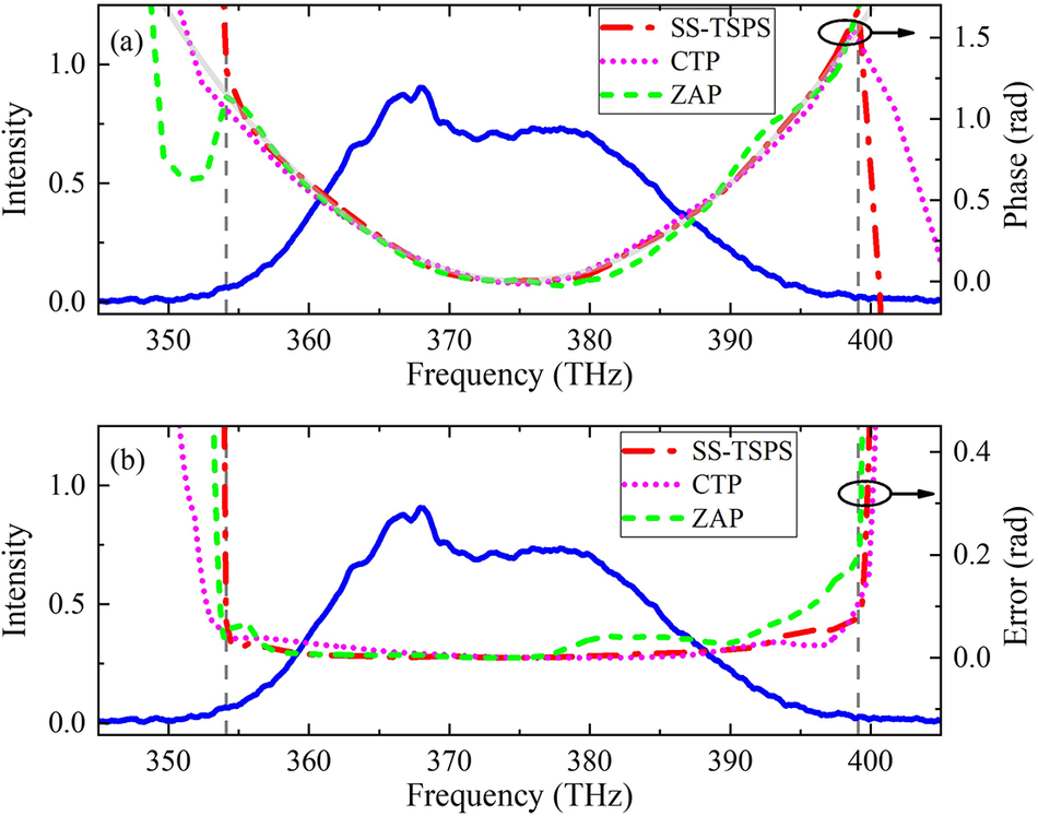
In order to experimentally measure the spectral phase induced by the test glass, all the SPIDER measurements have been made without and with glass in front of the setup. Figure 3(a) presents the retrieval spectral phases of the test glass measured by ZAP-SPIDER (green), CTP-SPIDER (orange) and SS-TSPS-SPIDER (red) together with the theoretical calculation (gray). On the whole, all of the measured phases agree well with the calculation range from 354.1 to 399.1 THz (gray dash vertical line), corresponding to the 10 dB bandwidth of the test spectrum (blue). In comparison to the orange and the red, the green deviates more obviously from the gray.
Measurement results of SS-TSPS, CTP and ZAP-SPIDERs with reference to the incident spectra (blue line). (a) The retrieved spectral phases and the corresponding theoretical curve (gray line). (b) The measured phase errors.

Figure 3 Long description
A two-panel attribute space diagram. Both panels share a common X-axis representing Frequency in T H z from 345 to 405 and a primary Y-axis on the left for Intensity from 0.0 to 1.0. A solid blue line representing the incident spectrum is consistent across both panels, showing a broad peak centered around 370 T H z.
Panel a: The right Y-axis measures Phase in rad from 0.0 to 1.5. A gray solid line represents the theoretical curve, forming a parabolic shape with a minimum at 375 T H z. Three retrieval curves are overlaid: a red dashed-dot line for S S - T S P S, a pink dotted line for C T P, and a green dashed line for Z A P. All three closely follow the theoretical gray line between the vertical dashed markers at 354 and 399 T H z, but diverge significantly outside this range.
Panel b: The right Y-axis measures Error in rad from 0.0 to 0.4. The three retrieval methods are plotted as phase error curves. Between 354 and 399 T H z, all three methods maintain a low, near-zero error. Outside this window, the error for all methods increases sharply, with the Z A P green dashed line showing a notable rise starting around 380 T H z compared to the others.
Figure 3(b) exhibits deviation curves between the measured and the calculated values of Figure 3(a) over the spectral range from 354.1 to 399.1 THz. The root-mean-square error (RMSE) is 33.8 mrad for the green, 14.1 mrad for the red and 16.1 mrad for the orange. One can see that the SS-TSPS-SPIDER has much smaller RMSE than that of ZAP-SPIDER, but comparable to that of CTP-SPIDER. The results reveal that our SS-TSPS-SPIDER has realized a very good combination of TSPS with single-shot mode, which can effectively suppress the background noise, thus improving the measured SNR and precision.
Table 1 summarizes the comparisons among SS-TSPS-SPIDER, CTP-SPIDER and ZAP-SPIDER based on our measurements. We can see that both SS-TSPS-SPIDER and CTP-SPIDER have higher accuracy, SNR and a wider measurable range than ZAP-SPIDER. ZAP-SPIDER can operate in single-shot mode, while CTP-SPIDER needs twice the operation, which makes it lose its real-time measurability. SS-TSPS-SPIDER can implement TSPS measurement under single-shot mode at the cost of space complexity and expense (two spectrometers).
The comparison of SS-TSPS, CTP and ZAP-SPIDER.

Table 1 Long description
The table compares three S P I D E R methods across seven technical parameters.
* S S dash T S P S: S N R is greater than 850. R M S E is 14.1 mrad. Precision is High. Range is 45 T H z. Method is Single shot. Spectrometer count is Two.
* C T P: S N R is greater than 850. R M S E is 16.1 mrad. Precision is High. Range is 45 T H z. Method is Two shots. Spectrometer count is One.
* Z A P: S N R is less than 250. R M S E is 33.8 mrad. Precision is Normal. Range is 35 T H z. Method is Single shot. Spectrometer count is One.
Footnotes indicate that R M S E and spectral range were measured for the spectral phase of a 3 millimeter thick B K 7 glass in the range from 354.1 to 399.1 T H z, with the range defined where the error is less than or equal to 60 mrad.
a The RMSE is measured for the spectral phase of a 3-mm-thick BK7 glass in the range from 354.1 to 399.1 THz.
b The spectral range is measured for the spectral phase of a 3-mm-thick BK7 glass when the error is
$<60\ \mathrm{mrad}$
 .
Figure 4 aims to check the single-shot measurement capability for the test pulse with the complex spectrum by comparing SS-TSPS-SPIDER and ZAP-SPIDER. Before entering into the setup, a 12-mm-thick BK7 glass is inserted into the beam path as the Kerr medium to complicate the test spectrum. As a result, the test spectrum becomes wider with some complex structures, so a small delay time (
$\tau =0.3\;\mathrm{ps})$
 was chosen between SFP-1 and SFP-2 for enough spectral sampling for spectral interference. However, the complex spectrum also leads to complex temporal structures both for the DC and the AC components, which results in nonnegligible overlapping among them, as shown in Figure 4(b) (blue line). Accordingly, it is impossible to pick out clearly one of the AC terms from the DC for ZAP-SPIDER. However, by using SS-TPSP-SPIDER, the tangled DC and some background noises can be greatly eliminated. Meanwhile, the AC amplitudes have been doubled, as seen from the red line.
Measurement results for the Kerr effect of SS-TSPS-SPIDER and ZAP-SPIDER: (a) recorded interferograms and (b) Fourier transform of the recorded interferograms.

Figure 4 Long description
The figure consists of two vertically stacked line graphs.
Top panel (a): The x-axis represents Frequency in T H z, ranging from 715 to 785. The y-axis represents Intensity, ranging from 0 to 8. A blue line labeled Spectral interferogram shows high-frequency oscillations across the spectrum, peaking near 745 T H z. A red line labeled Kerr spectrum shows a smoother, broader envelope that follows the general shape of the blue oscillations but without the rapid fluctuations.
Bottom panel (b): The x-axis represents Time in p s, ranging from minus 0.5 to 0.5. The y-axis represents Intensity, ranging from 0.0 to 1.2. A blue line labeled Z A P shows a sharp, dominant central peak at 0.0 p s reaching an intensity of 1.0, with two much smaller side peaks at approximately minus 0.3 p s and plus 0.3 p s. A red line labeled S S dash T S P S shows no central peak at 0.0 p s but features two distinct peaks at minus 0.3 p s and plus 0.3 p s, both reaching an intensity of approximately 0.5.
In Figure 5(a), the spectral phase is shown by the black line for ZAP-SPIDER, and by the red line for SS-TPSP-SPIDER. One can see that, from the spectral range from 359 to 386 THz (gray dash vertical lines), the black line is well overlapped with the red line. Once away from this zone, the black line begins to deviate from the red line, showing the obvious difference between the reconstructed spectral phases. Accordingly, as shown in Figure 5(b), the two SPIDER measurements present an obvious difference between the reconstructed temporal intensity and phase distributions, which is mainly attributed to the incomplete isolation of the DC from the AC terms.
Reconstructed electric-field for Kerr modulation by SS-TSPS and ZAP-SPIDERs. (a) Kerr spectrum and retrieved spectral phase. (b) Temporal intensity and phase.

Figure 5 Long description
Panel a is a line graph of Intensity and Phase rad versus Frequency T H z. The x-axis ranges from 330 to 420 T H z. The left y-axis is Intensity from 0.0 to 1.0, and the right y-axis is Phase rad from minus 2 to 4. A solid blue line represents the Kerr spectrum, peaking at approximately 368 T H z. Two phase curves are shown: a red dash-dot line for S S dash T S P S and a black dashed line for Z A P. Both phase curves follow a parabolic U-shape, reaching a minimum of 0 rad near 375 T H z and rising to approximately 2 rad at the frequency boundaries. Vertical dashed gray lines mark the region between 358 and 386 T H z.
Panel b is a line graph of Intensity and Phase rad versus Time f s. The x-axis ranges from minus 110 to 110 f s. The left y-axis is Intensity from 0.0 to 1.0, and the right y-axis is Phase rad from minus 8 to 4. The temporal intensity is shown by a solid blue line for S S dash T S P S and a solid black line for Z A P, both showing a main peak at 0 f s with smaller side lobes. The temporal phase is shown by a red dash-dot line for S S dash T S P S and a pink dotted line for Z A P. The S S dash T S P S phase shows a gradual increase from minus 8 rad at minus 100 f s to 0 rad at 110 f s, while the Z A P phase exhibits more oscillatory behavior between minus 8 and 2 rad.
5 Conclusion
Summarily, this paper presents a single-shot measurement by SPIDER combined with TSPS under single-shot mode, named SS-TSPS-SPIDER. Two spectral interferograms with π-phase shift by a single shot are captured by a design to combine and split the SFP pair with two orthogonal incident directions through a non-polarization splitter. Accordingly, SS-TSPS-SPIDER can experimentally remove the DC component exactly from the AC signals, which makes it have higher measurement accuracy. Equally important, SS-TSPS-SPIDER can not only cancel the background similar to the balance detection[ Reference Lu, Shen, Cao, Liao and Peng 27 ] but also increase the AC signal by a factor of two, thus greatly improving SNRs. Our experimental results show that SS-TSPS-SPIDER can measure the spectral dispersion of a 3-mm-thick BK7 glass with an error within 14.1 mrad over a range of around 45–375 THz, reflecting superior measurement accuracy compared with traditional SPIDER. The results also show the ability of SS-TSPS-SPIDER to measure ultrafast lasers with much more complex temporal/spectral pulse structures. Accordingly, this design provides a powerful method for the measurement of laser pulses, especially pulses at low repetition rate or in single-shot mode, and can be applied to characterize the temporal/spectral properties of ultra-intense and ultrashort laser pulses, which have been widely applied in extreme-physics frontiers such as strong-field physics and attosecond science.
Acknowledgements
This work is partially supported by the National Key R&D Program of China (Grant No. 2023YFA1608504), the National Natural Science Foundation of China (Grant Nos. 12174264, 92050203, 62275163, 62075138 and 61827815), the Natural Science Foundation of Guangdong Province (Grant Nos. 2024A1515010437 and 2024A1515011948) and the Shenzhen Fundamental Research Program (Grant Nos. JCYJ20240813141432042 and JCYJ20240813141423031).



 Open access

