1. Introduction
Natural convection in fluid-saturated porous media arises in an exceptionally wide range of physical and engineered systems. Representative examples include thermal management in heat exchangers, underground contaminant transport, the extraction of hydrocarbons, the dissolution of supercritical carbon dioxide sequestered in subsurface formations, the design of repositories for nuclear debris and thermal insulation, as well as broader processes involving heat storage and removal (Nield & Bejan Reference Nield and Bejan2017). In many of these settings, the physical properties of the saturating fluid – such as density, viscosity, specific heat and thermal expansion coefficient – depend strongly on temperature, and this dependence can markedly influence both the onset and subsequent evolution of buoyancy-driven convection.
In practical scenarios, it is often sufficient to assume constant fluid viscosity; however, in thermally stratified systems this simplification becomes untenable. Under such conditions, the temperature dependence of viscosity must be properly accounted for, especially for fluids exhibiting strong thermal sensitivity. Empirical evidence underscores this necessity (Rossby Reference Rossby1969): for water, a modest increase from 20 °C to 25 °C reduces viscosity by roughly 10 %, whereas thermal conductivity changes by less than 2 %. For 20 cSt silicone oil, the reduction is even steeper – nearly 20 % over the same temperature interval – with negligible change in conductivity. Across broader temperature ranges, the effect of viscosity variation can be far more pronounced; for instance, olive oil exhibits a decrease from 138 cP at 10 °C to 12.4 cP at 70 °C (Weast Reference Weast1988). These observations highlight that viscosity can vary by an order of magnitude across realistic temperature spans, whereas other fluid properties remain comparatively insensitive. This pronounced sensitivity of viscosity to temperature has motivated the development of numerous empirical and theoretical relations describing its temperature dependence. A variety of viscosity–temperature laws have consequently been proposed, each aiming to capture the essential thermoviscous behaviour with differing levels of fidelity. For many fluids, viscosity decreases approximately exponentially with increasing temperature. In regimes characterised by moderate temperature gradients, this exponential dependence is often well approximated by a linear relation, thereby facilitating analytical tractability. Palm, Ellingsen & Gjevik (Reference Palm, Ellingsen and Gjevik1967) employed a linear temperature-dependent viscosity model, in which the kinematic viscosity,
 $\nu (T)$
, is expressed as
 $\nu (T)=\nu _{0}\{1-\delta (T-T_{0})\}$
, with
 $\nu _{0}$
and
 $\delta$
being positive constants and
 $T_{0}$
a reference temperature. This model has been validated against experimental data for several fluids. For example, a least-squares fit to Rossby’s (Reference Rossby1969) data for water yields
 $\nu (T)=0.01008\{1-0.02199(T-20)\}$
, where
 $T$
is in °C and
 $\nu$
in cm2 s−1. Similarly, for 20 cSt silicone oil,
 $\nu (T)=0.21372\{1-0.02182(T-20)\}$
, which shows close agreement with experimental observations. Nevertheless, not all fluids conform well to a linear viscosity–temperature relationship. For instance, liquid sulphur and bismuth exhibit a maximum viscosity at a certain temperature, which can be represented by a quadratic relation
 $\nu (T)=\nu _{0}[1-\gamma (T-T_{0})^{2}]$
with
 $\gamma$
being constant, allowing the model to reproduce the observed temperature-dependent variation (Lide Reference Lide1991; Diaz & Straughan Reference Diaz and Straughan2004). Furthermore, an increasing body of experimental evidence supports the superior accuracy of an exponential relation
 $\nu (T)=\nu _{0}\exp [-\chi (T-T_{0})]$
with
 $\chi$
being constant, for many realistic fluids. For geophysical flows such as the Earth’s mantle convection, exponential viscosity–temperature dependence is commonly employed (Ogawa, Schubert & Zebib Reference Ogawa, Schubert and Zebib1991). Similarly, fluids like Golden Syrup, glycerol and polybutene exhibit ‘super-exponential’ behaviour (Booker Reference Booker1976; Stengel, Oliver & Booker Reference Stengel, Oliver and Booker1982; White Reference White1988).
Thermogravitational convection in porous media with variable viscosity plays a central role in a wide range of natural and technological processes, where the coupling between thermal gradients and viscosity variations strongly governs the onset and subsequent evolution of convective motion (Or Reference Or1989; Straughan Reference Straughan2004; Nield & Bejan Reference Nield and Bejan2017, and references therein). Classical studies have predominantly considered horizontal porous layers (Darcy–Bénard-type problems), yet vertically oriented layers bounded by impermeable walls and subjected to horizontal temperature gradients exhibit markedly different mechanisms. In such vertical systems, buoyancy acts along the vertical axis, and the resulting heat transfer and flow structure differ significantly from those in horizontal layers. Consequently, a detailed examination of thermal convection in vertical porous layers with variable viscosity is both timely and essential to advance understanding in this underexplored area. Kwok & Chen (Reference Kwok and Chen1987) examined separately the influence of no-slip velocity boundary conditions – introduced through Brinkman’s extension of the momentum equation – and of temperature-dependent viscosity under Darcy’s formulation. Their linear stability analysis revealed that both mechanisms can independently yield instability. Shankar, Nagamani & Shivakumara (Reference Shankar, Nagamani and Shivakumara2023a ) analysed the role of linear viscosity–temperature dependence and the Prandtl–Darcy number on the stability of buoyant flow in a vertical Darcy porous layer bounded by impermeable-isothermal walls. They reported unconditional stability for infinitesimal disturbances, consistent with the findings of Rees (Reference Rees1988) for constant viscosity. Extending this work, Shankar, Nagamani & Shivakumara (Reference Shankar, Nagamani and Shivakumara2023b ) explored nonlinear viscosity–temperature relationships, focusing on quadratic and exponential variations. The analysis showed that quadratic variations preserve flow stability, whereas exponential variations can induce instability under certain parametric conditions. In a subsequent study, the combined effects of linearly varying temperature-dependent viscosity and boundary permeability on the stability of natural convection in a vertical porous layer were considered by Shankar & Shivakumara (Reference Shankar and Shivakumara2024a ). It was demonstrated that the boundary permeability plays the dominant role in triggering instability, while viscosity variation primarily shifts the threshold once instability occurs.
In examining convective instability, the boundaries are most often idealised as either perfectly conducting (Dirichlet) or perfectly insulating (Neumann), corresponding respectively to fixed-temperature and fixed-flux conditions. In modelling thermal processes, however, boundary conditions play a decisive role. In practice, boundaries possess finite thermal conductivity and permit partial heat transfer with the surroundings – a situation particularly relevant in geophysical and engineering settings, where the thermal interaction is neither perfectly conductive nor ideally insulated. As such, Dirichlet and Neumann conditions correspond to extreme cases that cannot capture intermediate thermal behaviour. A more realistic representation is therefore achieved through Robin-type (mixed) boundary conditions, which incorporate finite interfacial conductivity and model convective exchange with the external environment via a uniform heat-transfer coefficient. The associated Biot number
 ${\textit{Bi}}$
quantifies the strength of this thermal coupling. Beyond their theoretical importance, Robin conditions have been widely employed to achieve closer agreement with experimental configurations and to model systems characterised by finite boundary conductivity. For instance, Robin-type cooling mechanisms have been shown to regulate convective instability in porous medium applications, such as metal casting and the solidification of binary alloys (Copley et al. Reference Copley, Giamei, Johnson and Hornbecker1970; Beckermann, Gu & Boettinger Reference Beckermann, Gu and Boettinger2000).
Following these foundational developments, the use of Robin boundary conditions in porous convection has gradually evolved through a series of landmark studies. The application of the Robin boundary conditions to the study of thermal convection in a porous medium was presented by Wilkes (Reference Wilkes1995), who considered a horizontal porous layer. Later, Kubitschek & Weidman (Reference Kubitschek and Weidman2003, Reference Kubitschek and Weidman2006) examined the effect of the Biot number on the onset of thermal instability in a horizontal porous layer, employing it to model boundary heat transfer induced by an external forced convection regime. Since then, numerous investigations have extended this approach to convection in porous rectangular domains, applying Robin conditions to the thermal perturbation either on the vertical boundaries, for instance, Nygård & Tyvand (Reference Nygård and Tyvand2010), or on the horizontal ones, as explored by Barletta & Storesletten (Reference Barletta and Storesletten2012). A notable advancement was achieved by Barletta, Tyvand & Nygård (Reference Barletta, Tyvand and Nygård2015), who incorporated Robin boundary conditions for both thermal and vertical velocity perturbations at the upper and lower boundaries. Their analysis revealed that Dirichlet conditions characterised by constant temperature or impermeability tend to impose the greatest constraint on the onset of convection, whereas Neumann conditions corresponding to insulated or free-slip boundaries are the least restrictive. Despite these developments, the application of Robin-type temperature conditions in a vertical porous layer remains comparatively unexplored.
The linear stability of buoyancy-driven flow in a vertical porous slab with Robin thermal boundary conditions and open lateral sides was analysed by Barletta, Celli & Ouarzazi (Reference Barletta, Celli and Ouarzazi2017), who showed that increasing the Biot number can exert both stabilising and destabilising effect on the base flow. Recently, Madhur, Shankar & Shivakumara (Reference Madhur, Shankar and Shivakumara2025) employed non-Dirichlet boundary conditions on the perturbation temperature field to study the stability of natural penetrative convection in a vertical porous layer. A novel finding of their study was the appearance of bi-modal or tri-modal neutral stability curves, indicating distinct onset modes arising from the combined effects of internal heat generation and the gradual transition of thermal boundary conditions from isothermal to adiabatic. Furthermore, increasing Biot number was found to promote an earlier onset of convection. Subsequently, Shankar, Mayur & Shivakumara (Reference Shankar, Mayur and Shivakumara2025) discussed the role of horizontal throughflow on thermoconvective instability in an unbounded vertical porous layer incorporating Robin thermal boundary conditions. It was noted that the magnitude of the Biot number discloses a new pathway for instability, with throughflow not only influencing its onset but also giving rise to different onset modes.
Motivated by these developments, a pragmatic modelling approach requires the inclusion of temperature-dependent viscosity laws and thermally imperfect boundary conditions to capture the realistic behaviour of natural convection in porous media. Such conditions are ubiquitous in geothermal systems and thermal energy-storage engineering, where the interplay between fluid rheology and boundary heat transfer governs the onset and evolution of convective motion. The present study, focused on a vertical porous layer, addresses a problem that, to the best of our knowledge, has not been received prior attention in the literature. The Robin thermal boundary conditions employed here naturally reduce to the Dirichlet (isothermal) form as the Biot number
 $Bi\rightarrow 0$
and to the Neumann (adiabatic) form as
 $Bi\rightarrow \infty$
, thereby encompassing the full spectrum of thermal boundary behaviours. Three forms of viscosity–temperature variations – namely, linear, quadratic and exponential – are considered. Given the assumption of a densely packed porous medium, the extended Darcy model is adopted to describe the flow. The stability of the base flow is analysed in both the infinite Prandtl–Darcy limit, where omission of the velocity time-derivative term implies an instantaneous adjustment of the velocity field to thermal forcing, and the finite Prandtl–Darcy regime, where retention of this term permits a finite response time during which the flow adjusts to temperature variations or externally imposed pressure gradients. The modal stability analysis is carried out numerically with a streamfunction–temperature formulation of the governing equations for the perturbations. Neutral stability curves and the critical values of the wavenumber, wave speed and the Darcy–Rayleigh number are determined for different prescribed values of the viscosity parameters, the Prandtl–Darcy number and the Biot number. The interplay among these parameters is systematically examined to elucidate their respective roles in promoting or suppressing buoyancy-driven instability. The streamlines and isotherms presented at the critical state demonstrate the development of a complex dynamics.
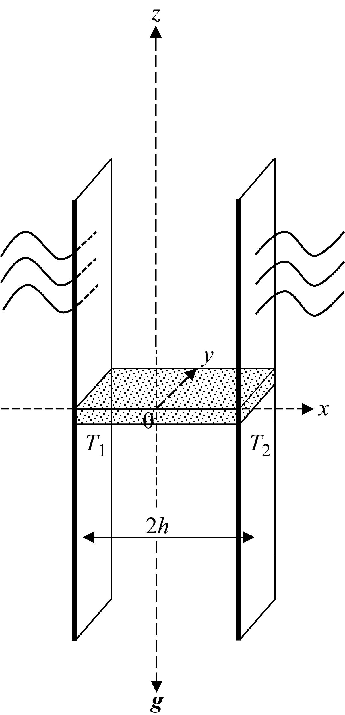
Vertical porous layer with external environment.

2. Mathematical formulation
As shown in figure 1, we consider an infinite vertical layer of an incompressible fluid-saturated homogeneous isotropic porous medium. The Cartesian coordinates
 $(x,y,z)$
are chosen so that
 $x$
is the horizontal coordinate normal to the vertical boundaries of the porous layer (the layer occupies
 $-h\leq x\leq h$
),
 $y$
is the spanwise coordinate (parallel to the vertical walls and unbounded) and
 $z$
is the vertical coordinate. The unit vector
 $\hat{\boldsymbol{k}}$
points upward, so that the gravitational acceleration is
 $\boldsymbol{g}=-g\hat{\boldsymbol{k}}$
. The impermeable vertical walls are subject to the thermal boundary conditions of the form (Straughan Reference Straughan2020)
 \begin{equation} \begin{array}{l} \beta \left[\frac{\partial T}{\partial x}-\frac{T_{2}-T_{1}}{2h}\right]h+\left(1-\beta \right)\left(T-T_{1}\right)=0\,\,\,{\textrm{at}}\,\,\,x=-h,\\[8pt] \beta \left[\frac{\partial T}{\partial x}-\frac{T_{2}-T_{1}}{2h}\right]h+\left(1-\beta \right)\left(T_{2}-T\right)=0\,\,\,{\textrm{at}}\,\,\,x=h, \end{array} \end{equation}
where
 $T$
is the temperature, and
 $T_{1}$
and
 $T_{2}$
are the constant temperatures at the left and right side surfaces of the porous layer, respectively, with
 $T_{2}\gt T_{1}$
. The boundary conditions involve a constant
 $\beta$
such that
 $0\leq \beta \lt 1$
. The case
 $\beta =0$
correspond to prescribed temperatures
 $T_{1}$
and
 $T_{2}$
(Dirichlet), whereas
 $\beta =1$
correspond to constant flux (Neumann). Thus, (2.1) represents Robin boundary conditions in their general form.
2.1. Governing equations
We model the fluid-saturated porous medium using a modified Darcy law, by invoking the validity of the Oberbeck–Boussinesq approximation. In this framework, the fluid density
 $\rho$
is taken to vary linearly with temperature,
 $\rho (T)=\rho _{0}[1-\alpha (T-T_{0})]$
, where
 $\alpha$
is the thermal expansion coefficient,
 $T_{0}=(T_{1}+T_{2})/2$
is the reference temperature and
 $\rho _{0}=\rho (T_{0})$
. The fluid viscosity
 $\mu$
is assumed to be temperature dependent in the following forms:
Case (i): Linear variation (Palm et al. Reference Palm, Ellingsen and Gjevik1967)
 \begin{equation}\mu \left(T\right)=\mu _{0}\left[1-\delta \left(T-T_{0}\right)\right].\end{equation}
Case (ii): Quadratic variation (Lide Reference Lide1991)
 \begin{equation}\mu \left(T\right)=\mu _{0}\left[1-\gamma \left(T-T_{0}\right)^{2}\right].\end{equation}
Case (iii): Exponential variation (Torrance & Turcotte Reference Torrance and Turcotte1971)
 \begin{equation} \mu (T)= {{\mu}_{0}}{\exp} [-\chi (T-T_{0})], \end{equation}
where
 $\mu _{0}$
is the viscosity at
 $T=T_{0}$
, while
 $\delta , \,\gamma$
and
 $\chi$
are positive constants. The analysis proceeds under the assumptions that local thermal equilibrium exists between the solid and the fluid, that viscous dissipation is negligible, and that no internal heating occurs within the porous medium. Under these conditions, the local mass, momentum and energy balance equations can be expressed as
 \begin{align} \boldsymbol{\nabla }\boldsymbol{\cdot }\boldsymbol{q} =0, \end{align}
 \begin{align} \frac{\rho _{0}}{\phi }\frac{\partial \boldsymbol{q}}{\partial t} =-\boldsymbol{\nabla }P +\rho \boldsymbol{g}-\frac{\mu \left(T\right)}{K}\boldsymbol{q}, \end{align}
 \begin{align} M\frac{\partial T}{\partial t}+\left(\boldsymbol{q}\boldsymbol{\cdot }\boldsymbol{\nabla }\right)T =\kappa {\nabla} ^{2}T, \end{align}
where
 $\boldsymbol{q}=(u,v,w)$
is the seepage velocity,
 $\phi$
is the porosity,
 $t$
is the time,
 $P$
is the pressure,
 $K$
is the permeability,
 $M$
is the ratio of heat capacities and
 $\kappa$
is the thermal diffusivity of the fluid.
The boundary conditions on velocity are
 \begin{equation}\boldsymbol{q}\boldsymbol{\cdot }\hat{\boldsymbol{i}}=0 \quad \text{at} \quad x=\pm h,\end{equation}
where
 $\hat{\boldsymbol{i}}$
is the unit vector along the
 $x$
-axis.
2.2. Dimensionless formulation
The mathematical model can be reformulated in dimensionless terms by scaling time, coordinates and fields as
 \begin{equation}\frac{h}{\kappa }\boldsymbol{q}\rightarrow \boldsymbol{q}, \!\quad\! \frac{\kappa }{Mh^{2}}t\rightarrow t, \!\quad\! h\boldsymbol{\nabla }\rightarrow \boldsymbol{\nabla }, \!\quad\! \frac{K}{\mu _{0}\kappa }P\rightarrow P, \!\quad\! \frac{T-T_{0}}{T_{2}-T_{1}}\rightarrow T, \!\quad\! \frac{1}{\mu _{0}}\mu \left(T\right)\rightarrow \mu \left(T\right),\end{equation}
which introduces the dimensionless parameters
 \begin{equation}R_{D}=\frac{\rho _{0}\alpha g(T_{2}-T_{1})Kh}{\mu _{0}\kappa }, \quad Pr_{D}=\frac{\mu _{0}\phi Mh^{2}}{\rho _{0}\kappa K}, \quad Bi=\frac{\beta }{(\beta -1)}.\end{equation}
Here,
 $R_{D}$
is the Darcy–Rayleigh number,
 ${\textit{Pr}}_{D}$
is the Prandtl–Darcy number and
 ${\textit{Bi}}$
is the Biot number. The viscosity laws in dimensionless form are given by
 \begin{equation}\mu \left(T\right)=1-\eta T, \quad \mu \left(T\right)=1-\varGamma T^{2}, \quad \mu \left(T\right)= {\exp} \left(-\Upsilon T\right),\end{equation}
where
 $\eta =\delta (T_{2}-T_{1}) , \Gamma =\gamma (T_{2}-T_{1})^{2}$
and
 $\Upsilon=\chi (T_{2}-T_{1})$
are the linear, quadratic and exponential viscosity parameters, respectively. Equations (2.9)–(2.11) allow one to rewrite the governing equations and the boundary conditions in a dimensionless form
 \begin{align} \boldsymbol{\nabla }\boldsymbol{\cdot }\boldsymbol{q} =0, \end{align}
 \begin{align}\frac{1}{Pr_{D}}\frac{\partial \boldsymbol{q}}{\partial t} =-\boldsymbol{\nabla }P+R_{D}T\hat{\boldsymbol{k}}-\mu \left(T\right)\boldsymbol{q}, \end{align}
 \begin{align} \frac{\partial T}{\partial t}+\left(\boldsymbol{q}\boldsymbol{\cdot }\boldsymbol{\nabla }\right) T={\nabla} ^{2}T, \end{align}
 \begin{align} \boldsymbol{q}\boldsymbol{\cdot }\hat{\boldsymbol{i}}=0 \quad \text{at} \quad x=\pm 1, \end{align}
 \begin{align} -Bi\left(\frac{\partial T}{\partial x}-\frac{1}{2}\right)+\left(T+\frac{1}{2}\right) & =0 \quad {\textrm{at}} \quad x=-1 \quad \text{ and } \quad \nonumber\\ Bi\left(\frac{\partial T}{\partial x}-\frac{1}{2}\right)+\left(T-\frac{1}{2}\right) & =0 \quad {\textrm{at}} \quad x=1. \end{align}
The validity of Squire’s theorem (Rees Reference Rees1988; Barletta Reference Barletta2015) justifies restricting the analysis to two-dimensional perturbations. Accordingly, the streamfunction
 $\psi (x,z,t)$
is introduced so that
 $(u,0,w)=(-\partial \psi /\partial z,0,\partial \psi /\partial x)$
and the pressure term is eliminated by applying the curl to (2.13). This procedure yields the following stability equations:
 \begin{align} \frac{1}{Pr_{D}}\frac{\partial }{\partial t}({\nabla} ^{2}\psi) =R_{D}\frac{\partial T}{\partial x}-\mu \left(T\right){\nabla} ^{2}\psi -\frac{\partial \mu \left(T\right)}{\partial x}\frac{\partial \psi }{\partial x}-\frac{\partial \mu \left(T\right)}{\partial z}\frac{\partial \psi }{\partial z}, \end{align}
 \begin{align} \frac{\partial T}{\partial t}+J\left(\psi ,T\right) ={\nabla} ^{2}T, \end{align}
where
 $J(\psi ,T)=({\partial \psi }/{\partial x})({\partial T}/{\partial z})-({\partial \psi }/{\partial z})({\partial T}/{\partial x})$
is the Jacobian.
The corresponding velocity boundary conditions, expressed in terms of the streamfunction, are
 \begin{equation}\psi =0 \quad \text{at} \quad x=\pm 1.\end{equation}
3. The basic stationary flow
Let us consider the basic state to be steady, one-dimensional and fully developed so that
 $\psi =\psi _{b}(x)$
and
 $T=T_{b}(x)$
, where the subscript
 $b$
denotes the basic state. Then (2.17) and (2.18), respectively become
 \begin{align} f\!(x)D^{2}\psi _{b}+Df\!(x)D\psi _{b} =R_{D}DT_{b}, \end{align}
 \begin{align} D^{2}T_{b} =0, \end{align}
where
 $D={\textrm{d}}/{\textrm{d}}x$
and
 $f\!(x)$
is the variable viscosity function. Solving (3.2) subject to the boundary conditions (2.16), we obtain
 \begin{equation}T_{b}=\frac{x}{2}.\end{equation}
It is noted that (3.3) coincides with the expression obtained directly by imposing the boundary conditions
 $T_{b}=\pm 1/2$
at
 $x=\pm 1$
. Now, the viscosity functions take the forms
 $f\!(x)=1-\eta x/2 , f\!(x)=1-\Gamma x^{2}/4$
and
 $f\!(x)=\exp (-\Upsilon x/2)$
corresponding to the linear, quadratic and exponential variations of viscosity, respectively. With these forms of
 $f\!(x)$
, (3.1) is solved analytically subject to the boundary conditions (2.19), leading to the basic streamfunction
 \begin{align} \psi _{b} =\frac{R_{D}\left[{\log} \left(2+\eta \right)\left(x-1\right)+2{\log} \left(2-\eta x\right)-{\log} \left(2-\eta \right)\left(x+1\right)\right]}{{\eta} \left[{\log} \left(2-\eta \right)-{\log} \left(2+\eta \right)\right]}, \end{align}
 \begin{align} \psi _{b} =\frac{R_{D}\left[{\log} \left(4-\varGamma \right)-{\log} \left(4-\varGamma x^{2}\right)\right]}{\varGamma }, \end{align}
and
 \begin{equation}\psi _{b}=\frac{R_{D}\left\{2e^{\Upsilon /2}+e^{\Upsilon x/2}\left[e^{\Upsilon }\left(x-1\right)-x-1\right]\right\}}{\Upsilon \left(e^{\Upsilon }-1\right)},\end{equation}
for the linear, quadratic and exponential cases, respectively. In the limit
 $\eta \rightarrow 0 ,\, \Gamma \rightarrow 0$
and
 $\Upsilon\rightarrow 0$
, (3.4)–(3.6) reduce to
 $\psi _{b}=R_{D}(x^{2}-1)/4$
, which recovers the classical constant viscosity case with appropriate scaling (Rees Reference Rees2011).
4. Linearised perturbation dynamics
The onset of instability is studied by perturbing the basic state in the form
 \begin{equation}\psi =\psi _{b}+\varepsilon \hat{\psi }, \quad T=T_{b}+\varepsilon \hat{T},\end{equation}
where
 $\varepsilon \gt 0$
is a perturbation parameter and
 $\hat{\psi }$
and
 $\hat{T}$
are the perturbation contributions to the streamfunction and temperature fields, respectively. The linear stability analysis is carried out by substituting (4.1) into (2.16)–(2.19) and by neglecting the terms
 $O(\varepsilon ^{2})$
. We then obtain
 \begin{align} \frac{1}{Pr_{D}}\frac{\partial }{\partial t}({\nabla} ^{2}\hat{\psi }) & =R_{D}\frac{\partial \hat{T}}{\partial x}-f\!(x){\nabla} ^{2}\hat{\psi }-Df\!(x)\left[2D^{2}\psi _{b}\hat{T}+2D\psi _{b}\frac{\partial \hat{T}}{\partial x}+\frac{\partial \hat{\psi }}{\partial x}\right] \nonumber\\ & \quad -\, 2D^{2}f\!(x)D\psi _{b}\hat{T}, \end{align}
 \begin{align} \frac{\partial \hat{T}}{\partial t} ={\nabla} ^{2}\hat{T}-D\psi _{b}\frac{\partial \hat{T}}{\partial z}+\frac{1}{2}\frac{\partial \hat{\psi }}{\partial z}, \end{align}
 \begin{align} \hat{\psi } =\hat{T}\pm Bi\frac{\partial \hat{T}}{\partial x}=0 \quad \text{at} \quad x=\pm 1. \end{align}
4.1. Normal mode analysis
We now focus on dynamics of normal modes expressed as
 \begin{equation}(\hat{\psi },\hat{T})(x,z,t)=(\varPsi ,\varTheta )(x)e^{ia(z-ct)}, \quad \text{with} \quad a\in {\mathbb{R}},c\in \mathbb{C},\end{equation}
where
 $a$
is the wavenumber and
 $c(=c_{r}+ic_{i})$
is a wave speed. The phase velocity is the real part of
 $c$
, while the temporal growth rate is the imaginary part of
 $c$
. Substituting (4.5) into (4.2)–(4.4), one obtains
 \begin{align} & f\!(x) (D^{2}-a^{2})\varPsi + Df\!(x) (2D^{2}\psi _{b}\varTheta +2D\psi _{b}D\varTheta +D\varPsi ) \nonumber\\ & \quad+\, 2D^{2}f\!(x)D\psi _{b}\varTheta -R_{D}D\varTheta =\frac{iac}{Pr_{D}}(D^{2}-a^{2})\varPsi , \end{align}
 \begin{align} (D^{2}-a^{2})\varTheta +ia\left(\frac{1}{2}\varPsi -D\psi _{b}\varTheta \right) =-iac\varTheta , \end{align}
 \begin{align} \varPsi =\varTheta \pm BiD\varTheta =0 \quad & \text{at} \quad x=\pm 1. \end{align}
5. Computation of the eigenvalue
The Chebyshev collocation method (Canuto et al. Reference Canuto, Hussaini, Quarteroni and Zang1987; Shankar & Shivakumara Reference Shankar and Shivakumara2022, Reference Shankar and Shivakumara2024b , Reference Shankar and Shivakumara2024c ) is employed to discretise the linear disturbance (4.6) and (4.7) together with the boundary conditions (4.8), leading to the formulation of a generalised eigenvalue problem of the form
 \begin{equation}\boldsymbol{AX}=c\boldsymbol{BX}.\end{equation}
Here,
 $\boldsymbol{A}$
and
 $\boldsymbol{B}$
are square complex matrices, while
 $c$
and
 $\boldsymbol{X}$
denote the eigenvalue and the eigenvector, respectively. The eigenvalues of the matrix pencil
 $(\boldsymbol{A},\boldsymbol{B})$
are computed using the QZ algorithm (Moler & Stewart Reference Moler and Stewart1973), implemented through MATLAB’s built-in routines.
6. Results and discussion
The onset of convection in a vertical Darcy porous slab is analysed by considering different temperature-dependent viscosity models and imperfect thermal boundary conditions. For linearly and quadratically varying viscosity, the parameters
 $\eta$
and
 $\Gamma$
must satisfy
 $0\lt \eta \lt 2$
and
 $0\lt \Gamma \lt 4$
, respectively, to ensure that the viscosity remains positive. In contrast, exponential viscosity variation, characterised by the parameter
 $\Upsilon$
, imposes no such restriction, allowing
 $\Upsilon$
to take any non-negative value. In practical situations,
 $\Upsilon$
typically spans from
 $O(1)$
for weakly temperature-sensitive fluids – such as silicone oils and glycerine – to
 $O(10{-}30)$
for materials exhibiting strong thermal softening, including molten silicates and mantle rocks. Scaling arguments based on realistic activation energies and geothermal temperature gradients yield
 $\Upsilon \approx 15{-}20$
, corresponding to viscosity contrasts of several orders of magnitude across the convecting layer. Consequently, the range
 $0\leq \Upsilon \leq 25$
adopted in the present study bridges the regimes relevant to both laboratory fluids and natural convective systems. The Biot number
 ${\textit{Bi}}$
characterises the thermal boundary conditions, with
 $Bi=0$
corresponding to perfectly isothermal (Dirichlet) walls,
 $Bi\rightarrow \infty$
to adiabatic (Neumann) walls and intermediate values to partially conducting boundaries.
In the Darcy formulation, the infinite Prandtl–Darcy number limit (
 ${\textit{Pr}}_{D}\rightarrow \infty$
) is frequently invoked, whereby the time-derivative term in the momentum equation is suppressed. This approximation (Straughan Reference Straughan2008; Nield & Bejan Reference Nield and Bejan2017) rests on the physical basis that the strong viscous resistance of the pore matrix damps velocity fluctuations on time scales far shorter than those of thermal diffusion. The velocity field therefore adjusts almost instantaneously to buoyancy and pressure forcing and can be regarded as slaved to the evolving thermal field; this case is referred to as Model I. While the finite-
 ${\textit{Pr}}_{D}$
assumption, denoted Model II, captures unsteady effects in the momentum balance and hence captures the essential physics of the onset of convective instability. Physical estimates across a range of porous media show that
 ${\textit{Pr}}_{D}$
often attains values of order unity or larger, so Model II is required for realistic stability predictions (Vadasz Reference Vadasz1998). For example, in a mushy layer formed during binary alloy solidification, with typical values
 $Pr=10^{-3}$
(liquid metals),
 $\phi =0.1,Da=10^{-4}$
and
 $M=1.2$
, one obtains
 ${\textit{Pr}}_{D}=1.2$
; in a fractured porous medium with
 $Pr=7$
(water),
 $\phi =Da=10^{-2}$
and
 $M=1.2$
, the value rises to
 ${\textit{Pr}}_{D}=8.4$
, whereas with
 $Pr=10^{2}$
(oil),
 $\phi =10^{-2}, Da=10^{-3}$
and
 $M=1.2$
, it reaches
 ${\textit{Pr}}_{D}=1200$
. These values clearly show that neglecting
 ${\textit{Pr}}_{D}$
is not universally valid, and that it must be retained in the Darcy momentum equation, since finite values may exert a significant influence on the stability characteristics of the flow. In what follows, both regimes are examined: § 6.1 addresses the infinite-
 ${\textit{Pr}}_{D}$
limit, while § 6.2 treats finite-
 ${\textit{Pr}}_{D}$
, thereby providing a unified framework that spans the full spectrum of physically realisable scenarios.
Growth rate
 $c_{i}$
versus wavenumber
 $a$
for different (a)
 $\eta$
with
 $Bi=1 , R_{D}=10^{3}$
, (b)
 ${\textit{Bi}}$
with
 $\eta =1.5 , R_{D}=10^{3}$
and (c)
 $R_{D}$
with
 $\eta =1.5 , Bi=10$
.

6.1. Model I
6.1.1. Analysis of the growth rate
Figures 2(a–c), 3(a–c) and 4(a–d) depict the variation of the growth rate
 $c_{i}$
as a function of the wavenumber
 $a$
for different values of the governing parameters, corresponding to linear, quadratic and exponential viscosity–temperature laws, respectively. The sign of
 $c_{i}$
provides the stability criterion:
 $c_{i}\lt 0$
denotes stability, while
 $c_{i}\gt 0$
signals instability. The results are computed using
 $N=50$
, where
 $N$
is the number of Chebyshev collocation points, for which the numerical method achieves convergence of the maximum temporal growth rate
 $c_{i}$
to four-decimal accuracy across all parameter sets (table not shown). Figures 2 and 3 show that
 $c_{i}\lt 0$
in all cases examined, thereby demonstrating that instability is precluded irrespective of the nature of thermal boundaries. This conclusion aligns precisely with the seminal work of Gill (Reference Gill1969), who established the unconditional stability of the natural convection parallel flow in a vertical porous slab with constant viscosity and isothermal boundaries.
Growth rate
 $c_{i}$
versus wavenumber
 $a$
for different (a)
 $\Gamma$
with
 $Bi=10 , R_{D}=10^{3}$
, (b)
 ${\textit{Bi}}$
with
 $\Gamma =3 , R_{D}=10^{3}$
and (c)
 $R_{D}$
with
 $\Gamma =3 , Bi=10$
.

Growth rate
 $c_{i}$
versus wavenumber
 $a$
for different
 $\Upsilon$
with (a)
 $Bi=1 , R_{D}=10^{3}$
, (b)
 $Bi=10 , R_{D}=10^{3}$
, (c)
 $Bi=10^{2} , R_{D}=10^{3}$
and (d)
 $Bi=10^{2} , R_{D}=10^{2}$
.

When the viscosity instead varies exponentially with temperature, the behaviour changes markedly (figure 4
a–d). Under specific parametric conditions, the sign of
 $c_{i}$
switches from negative to positive, indicating the emergence of instability. The figures reveal that the possibility of instability is closely tied to the values of
 $\Upsilon, Bi$
and
 $R_{D}$
. For instance, when
 $Bi=1$
and
 $R_{D}=10^{3} , c_{i}$
remains negative for all
 $\Upsilon$
(figure 4
a), confirming stability. As
 ${\textit{Bi}}$
increases to 10 (figure 4
b) and 100 (figure 4
c),
 $c_{i}$
attains positive value at sufficiently high
 $\Upsilon$
. Likewise, increase in either
 ${\textit{Bi}}$
(figure 4
b,c) or
 $R_{D}$
(figure 4
c,d) promotes instability at progressively lower values of
 $\Upsilon$
. Thus, the stability of the base flow is strongly influenced by the viscosity laws, with exponential dependence producing instabilities that do not occur under linear or quadratic variations.
6.1.2. The neutral stability curves
The solution of (4.6)–(4.8) yields the neutral stability boundaries for the case of exponentially varying viscosity, represented in the
 $(a,R_{D})$
-plane. Along these curves, the perturbation growth rate vanishes, defining the threshold of marginal stability. Of particular interest is the point on each curve corresponding to the lowest
 $R_{D}$
for specified
 ${\textit{Bi}}$
and
 $\Upsilon$
, which marks the onset of instability. Typically, the curve exhibits an absolute minimum at a wavenumber
 $a$
; this value defines the critical wavenumber
 $a_{c}$
and the corresponding Darcy–Rayleigh number
 $R_{\textit{Dc}}$
that govern the transition to instability.
A convergence study is carried out to assess the sensitivity of the critical triplets (
 $R_{\textit{Dc}} , a_{c} , c_{c}$
) to variations in
 $N$
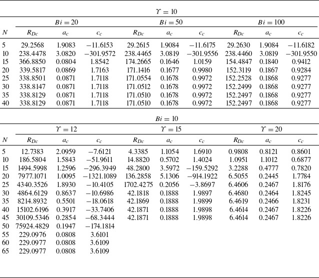
. Table 1 reports representative results for selected combinations of
 ${\textit{Bi}}$
and
 $\Upsilon$
, which serve as a benchmark for the present set-up and provide a reliable reference for future studies and comparative analyses. The data demonstrate that increasing
 $N$
significantly improves the accuracy of the computed critical values, achieving precision of four decimal places for sufficiently large
 $N$
. The results further indicate that
 $N=70$
is adequate to capture the critical stability parameters with high reliability. Accordingly, this value of
 $N$
is adopted in calculating the critical parameters to ensure computational efficiency without loss of accuracy.
Selected convergence test results for the Chebyshev collocation method in the limit
 ${\textit{Pr}}_{D}\rightarrow \infty$
.

Figures 5(a) and 5(b) present the neutral stability curves in the
 $(a,R_{D})$
-plane for different
 ${\textit{Bi}}$
when
 $\Upsilon=8.5$
and
 $\Upsilon=10$
, respectively. The plots reveal that decreasing
 ${\textit{Bi}}$
promotes flow stabilisation, as evidenced by the upward and leftward displacement of the neutral curves. A notable feature is the widening gap between the minima of the curves for
 $Bi=100$
and
 $Bi=200$
, which is considerably larger than that between
 $Bi=300$
and
 $Bi=400$
in both figures. This behaviour reflects a progressive steepening of the neutral stability boundary as
 ${\textit{Bi}}$
decreases. The underlying mechanism is set by the thermal resistance of the bounding walls. At low
 ${\textit{Bi}}$
, the walls are relatively conducting, so the system is highly sensitive to changes in wall heat loss: increasing
 ${\textit{Bi}}$
reduces leakage and rapidly lowers the instability threshold
 $R_{\textit{Dc}}$
. At high
 ${\textit{Bi}}$
, the walls behave nearly adiabatically, and further increases have only a marginal effect on heat transfer. This transition – from strong sensitivity at moderate
 ${\textit{Bi}}$
to near saturation at large
 ${\textit{Bi}}$
-accounts – for the progressively smaller displacements of the neutral curves and underlies the observed non-monotonic variation in curve spacing. Moreover, the comparison between figures 5(a) and 5(b) indicates that, for a fixed
 ${\textit{Bi}}$
, increasing
 $\Upsilon$
leads to an earlier onset of instability, with lower values of
 $R_{\textit{Dc}}$
. The Biot number ranges considered in each figure also vary to reflect the sensitivity of instability to
 $\Upsilon$
: for
 $\Upsilon=8.5$
, the chosen range of
 ${\textit{Bi}}$
is
 $80{-}450$
, whereas for
 $\Upsilon=10$
, the instability range expands considerably to
 $20{-}450$
. This variation gives emphasis to the critical role of
 $\Upsilon$
in shaping the parametric domain where instability occurs. Furthermore, the transition to instability occurs only through travelling-wave modes. This means that the neutral stability curves, defined by a zero imaginary part of
 $c$
, are also characterised by a non-zero real part of
 $c$
, so that the phase velocity of the neutrally stable modes is non-zero. This behaviour originates from the cross-stream non-uniformity of the base vertical velocity induced by the exponential viscosity law: near the heated wall, the sharp decrease in viscosity produces steep velocity gradients and hence larger upward basic velocity, whereas nearer the cooler wall the higher viscosity suppresses the flow. As a result, different portions of a disturbance are advected at unequal vertical speeds, generating a systematic phase shift between velocity and temperature perturbations. This precludes a neutrally balanced standing mode; neutrality is attained only when the disturbance propagates as a travelling wave with finite phase speed.
Neutral stability curves for (a)
 $\Upsilon=8.5$
and (b)
 $\Upsilon=10$
with different values of
 ${\textit{Bi}}$
.

6.1.3. Linear stability boundaries
The critical stability parameters are illustrated in figures 6(a), 6(b) and 6(c), capturing the variation of
 $R_{\textit{Dc}} , a_{c}$
and
 $c_{c}$
, respectively, against
 ${\textit{Bi}}$
for various
 $\Upsilon$
values. Figure 6(a) clearly demonstrates that instability is confined to a finite range of
 ${\textit{Bi}}$
, a phenomenon consistently observed across all examined values of
 $\Upsilon$
. This arises because both excessive wall conduction and near-adiabatic insulation suppress buoyant amplification: at small
 ${\textit{Bi}}$
, highly conducting walls overdamp thermal perturbations by leaking heat too efficiently, whereas at very large
 ${\textit{Bi}}$
, nearly adiabatic boundaries block vertical heat flux. Consequently, instability can develop only within an intermediate
 ${\textit{Bi}}$
range where the opposing effects of conduction and insulation are balanced. Exponential viscosity–temperature dependence fundamentally modifies this balance: the steep viscosity decrease near the heated wall amplifies buoyant forcing. This counteracts the damping effect of wall heat conduction and allows instability to persist at progressively lower
 ${\textit{Bi}}$
. As a result, the lower
 ${\textit{Bi}}$
cutoff shifts downward with increasing viscosity parameter
 $\Upsilon$
, while its upper cutoff remains nearly unchanged because instability in the near-adiabatic regime already relies on the internal temperature contrast. The outcome is an asymmetric broadening of the instability window, dominated by the reduction of its lower bound. Within this instability bandwidth, increasing
 ${\textit{Bi}}$
and
 $\Upsilon$
lowers
 $R_{\textit{Dc}}$
, thereby advancing the onset of instability. Thus, the emergence of instability is attributed solely to the combined influence of exponentially varying viscosity and thermally imperfect boundary conditions. Importantly, neither mechanism alone is sufficient to make the system unstable.
Critical values of (a)
 $R_{D}$
, (b)
 $a$
and (c)
 $c$
versus
 ${\textit{Bi}}$
for different
 $\Upsilon$
.

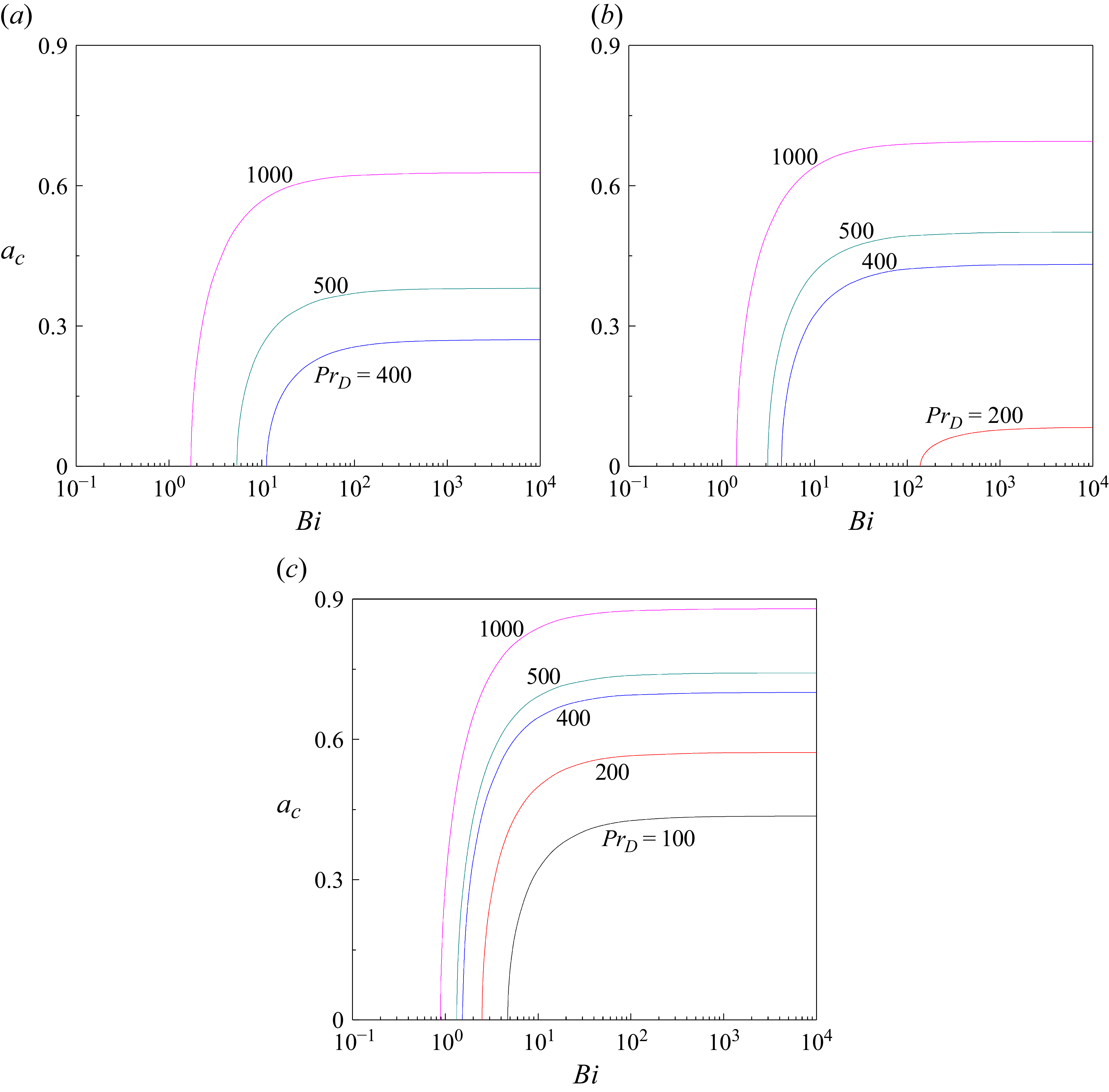
Figure 6(b) reveals that the onset of instability is accompanied by an increase in the critical wavenumber
 $a_{c}$
with increasing
 ${\textit{Bi}}$
, signifying a contraction in the size of convection cells. A similar trend occurs with increasing
 $\Upsilon$
. The associated values of
 $c_{c}$
are displayed in figure 6(c), highlighting distinct behaviours based on the magnitude of
 $\Upsilon$
. For
 $\Upsilon=8.21,8.25,8.3,8.5,9$
and
 $9.1, c_{c}$
increases with
 ${\textit{Bi}}$
, while for
 $\Upsilon=10$
, 15 and 20, the trend is entirely reversed. The sign of
 $c_{c}$
determines the drift direction: for
 $\Upsilon \leq 9 , c_{c}\lt 0$
and the cells propagate downward, while for larger
 $\Upsilon, c_{c}\gt 0$
and they move upward, for all
 ${\textit{Bi}}$
. The case
 $\Upsilon=9.1$
is exceptional, with
 $c_{c}$
changing sign from negative to positive as
 ${\textit{Bi}}$
increases, indicating a transition from downward to upward motion of the convection cells. This switch reflects the competition between buoyant forcing near the hot wall and viscous resistance imposed by the cold sublayer, mediated by the basic flow structure. For
 $\Upsilon \in [8.21,9]$
, the viscosity contrast is significant, yet the eigenfunctions extend across the layer, so the cold side damps upward motion and biases drift downward (
 $c_{c}\lt 0$
). As
 $\Upsilon$
increases, the exponential mobility contrast sharpens the basic flow shear and progressively localises the neutral mode near the hot wall (‘hot wall locking’). Once this localisation is strong enough (
 $\Upsilon \gtrsim 10$
), buoyant anomalies at the hot side rise with minimal resistance, and drift reorients from downward to upward
 $(c_{c}\gt 0).$
Near the cross-over (
 $\Upsilon=9.1$
), the outcome depends sensitively on
 ${\textit{Bi}}$
: increasing
 ${\textit{Bi}}$
reduces wall heat exchange, reinforcing hot-side buoyancy anomalies, thereby triggering the negative-to-positive flip of
 $c_{c}$
.
The insights gained from figure 6 motivate the presentation of
 $R_{\textit{Dc}} , a_{c}$
and
 $c_{c}$
as a function of
 $\Upsilon$
for different
 ${\textit{Bi}}$
, as portrayed in figures 7(a), 7(b) and 7(c), respectively. These plots serve two purposes: first, to identify precisely the threshold value of
 $\Upsilon$
at which the instability sets in, and second, to pinpoint the value of
 $\Upsilon$
at which c
c
changes sign, thereby elucidating the response of the critical stability parameters at this value of
 $\Upsilon$
. Figure 7(a) shows that, for each
 ${\textit{Bi}}$
, there exists a threshold
 $\Upsilon$
, say
 $\tilde{\Upsilon}$
, below which the flow remains stable, as all perturbations exhibit negative growth rates because viscosity variations are too weak to promote instability. Notably,
 $\tilde{\Upsilon}$
increases as
 ${\textit{Bi}}$
decreases. For all
 ${\textit{Bi}}$
, a pronounced decline in
 $R_{\textit{Dc}}$
is observed as
 $\Upsilon$
increases (figure 7
a), while the corresponding
 $a_{c}$
increases (figure 7
b). The behaviour of
 $c_{c}$
with
 $\Upsilon$
depends strongly on
 ${\textit{Bi}}$
: it remains positive for
 ${\textit{Bi}}$
= 5, 10 and 20, but for
 ${\textit{Bi}}$
= 50, 100 and 200,
 $c_{c}$
changes sign from negative to positive as
 $\Upsilon$
increases (figure 7
c). The variation of
 $c_{c}$
with
 $\Upsilon$
across different
 ${\textit{Bi}}$
reflects the competition between buoyancy forcing near the hot wall and viscous resistance near the cold side, as mentioned in figure 6(c). For small
 ${\textit{Bi}}$
, buoyancy at the hot wall dominates and
 $c_{c}$
remains positive. At large
 ${\textit{Bi}}$
, reduced thermal confinement weakens buoyancy at the hot wall, so cold side viscous resistance dominates and drives
 $c_{c}$
negative. As
 $\Upsilon$
increases, viscosity contrast intensifies hot wall localisation, restoring positive drift. A key distinction from earlier studies (Madhur et al. Reference Madhur, Shankar and Shivakumara2025; Shankar et al. Reference Shankar, Mayur and Shivakumara2025) is that the sign change of
 $c_{c}$
was accompanied by abrupt jumps in
 $R_{\textit{Dc}},\,a_{c}$
and in
 $c_{c}$
itself, signalling the emergence of distinct new onset modes; in contrast, no such jumps are observed in the present study, where
 $c_{c}$
changes sign smoothly.
Critical values of (a)
 $R_{D}$
, (b)
 $a$
and (c)
 $c$
versus
 $\Upsilon$
for different
 ${\textit{Bi}}$
.

6.1.4. Stability and instability zone
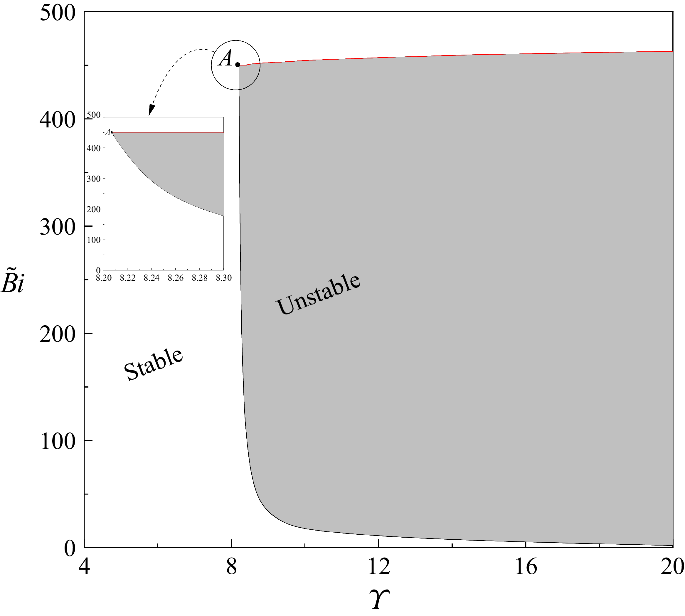
Figure 8 provides an overall view of the stable and unstable regions in the (
 $\Upsilon, \tilde{B}i$
)-plane. The grey-shaded region denotes instability, while the surrounding white region corresponds to stability. It is evident from the figure that, for any fixed value of
 $\Upsilon$
within the instability region, two distinct bounds of
 $\tilde{B}i$
are identified: the lower bound marks the onset of instability and the upper bound signifies the return to stability. Instability is therefore confined to a finite interval of
 $\tilde{B}i$
, revealing a well-defined window in which perturbations grow with time. The two bounds of
 $\tilde{B}i$
coalesce at point
 $A$
, identified at
 $\Upsilon$
= 8.2070. This coalescence signals the emergence of instability, which occurs only when
 $\Upsilon \geq 8.2070$
. For
 $\Upsilon \gt 8.2070$
, the unstable region broadens with increasing
 $\Upsilon$
, forming a widening band in the (
 $\Upsilon, \tilde{B}i$
)-plane. The lower bound of
 $\tilde{B}i$
decreases steadily with
 $\Upsilon$
, tending asymptotically to zero, while the upper bound increases only slightly. Finally, it should be noted that the lower bound of
 $\tilde{B}i$
, corresponding to
 $R_{\textit{Dc}}\rightarrow \infty$
and
 $a_{c}\rightarrow 0$
, is obtained by solving the stability eigenvalue problem over a wide range of
 $R_{D}$
, where numerical accuracy becomes considerably reduced.
Stable and unstable zones in the (
 $\Upsilon,\,\tilde{B}i$
)-plane.

6.1.5. Streamlines and isotherms
A qualitative depiction of streamlines and isotherms in the
 $(x,z)$
-plane under critical conditions,
 $R_{D}=R_{\textit{Dc}} , a=a_{c}$
and
 $c=c_{c}$
, is presented in figures 9 and 10 for different values of
 ${\textit{Bi}}$
and
 $\Upsilon$
, respectively. By looking at these figures, the shape of the convective cells and their space distribution along the slab can be visualised, providing clearer insight into the effect of the imperfectly conducting boundaries and variable viscosity on the flow dynamics. The time variable is omitted from the figure captions (equivalently, set to
 $t=0$
), as its inclusion would merely induce a phase shift of the patterns along the vertical
 $z$
-axis without altering the physical structure. Additionally, the vertical coordinate
 $z$
is rescaled in each figure to correspond to one full wavelength,
 $2\pi /a_{c}$
, ensuring consistency of spatial representation across all considered values of
 $\Upsilon$
and
 ${\textit{Bi}}$
. In all the plots, blue contours denote negative values (counterclockwise rotation), whereas red contours indicate positive values (clockwise rotation). As exemplified in figure 9(a), the streamlines adhere closely to the right boundary, indicating the dominance of convective motion adjacent to the heated wall. The isotherms stretch from the hot wall toward the cold wall and gradually flatten near the latter owing to the weak horizontal temperature gradient and the corresponding circulation cells remain open near the cold boundary, consistent with this temperature distribution (figure 9
e). This overall pattern of streamlines (figure 9
b–d) and isotherms (figure 9
f–h) remains largely unaffected with increasing
 ${\textit{Bi}}$
. Figure 10(a–d) reveals that the streamlines compress progressively toward the hot boundary as
 $\Upsilon$
increases. The corresponding isotherms are likewise compressed toward the hot wall, clinging more tightly to it and losing horizontal reach (figure 10
e–h).
Streamlines (a–d) and isotherms (e–h) of the perturbation modes at the onset of instability for
 $\Upsilon=10$
with different
 ${\textit{Bi}}$
at a fixed
 $t$
.

Streamlines (a–d) and isotherms (e–h) isotherms of the perturbation modes at the onset of instability for
 $Bi=10$
with different
 $\Upsilon$
at a fixed
 $t$
.

6.2. Model II
This section investigates the influence of the finite Prandtl–Darcy number
 ${\textit{Pr}}_{D}$
on the stability characteristic of the system. The analysis spans
 $1\leq Pr_{D}\leq 10^{3}$
, while the parameter ranges of
 ${\textit{Bi}}$
and the three forms of viscosity parameters are retained as before. The computations carried out for a wide range of
 $\eta /\Gamma /\Upsilon, Bi$
and
 ${\textit{Pr}}_{D}$
reveal that, for certain parameter combinations, the growth rate
 $c_{i}$
undergoes a sign reversal from negative to positive, thereby confirming the emergence of instability in all the viscosity–temperature laws. This behaviour contrasts with Model I, where instability arises only for the exponential viscosity law. To avoid redundancy, growth rate and neutral stability curves are omitted, and attention is restricted to the stability boundaries, which provide a clearer depiction of the onset of instability. Much of the underlying physics follows that discussed in § 6.1 and is not repeated here. It is noted that the same value of
 $N=70$
used in Model I is also adopted here for calculating the critical parameters, as it yields numerically consistent results for all three viscosity–temperature relations. This conclusion is supported by convergence tests performed over a broad set of governing parameters (table not shown).
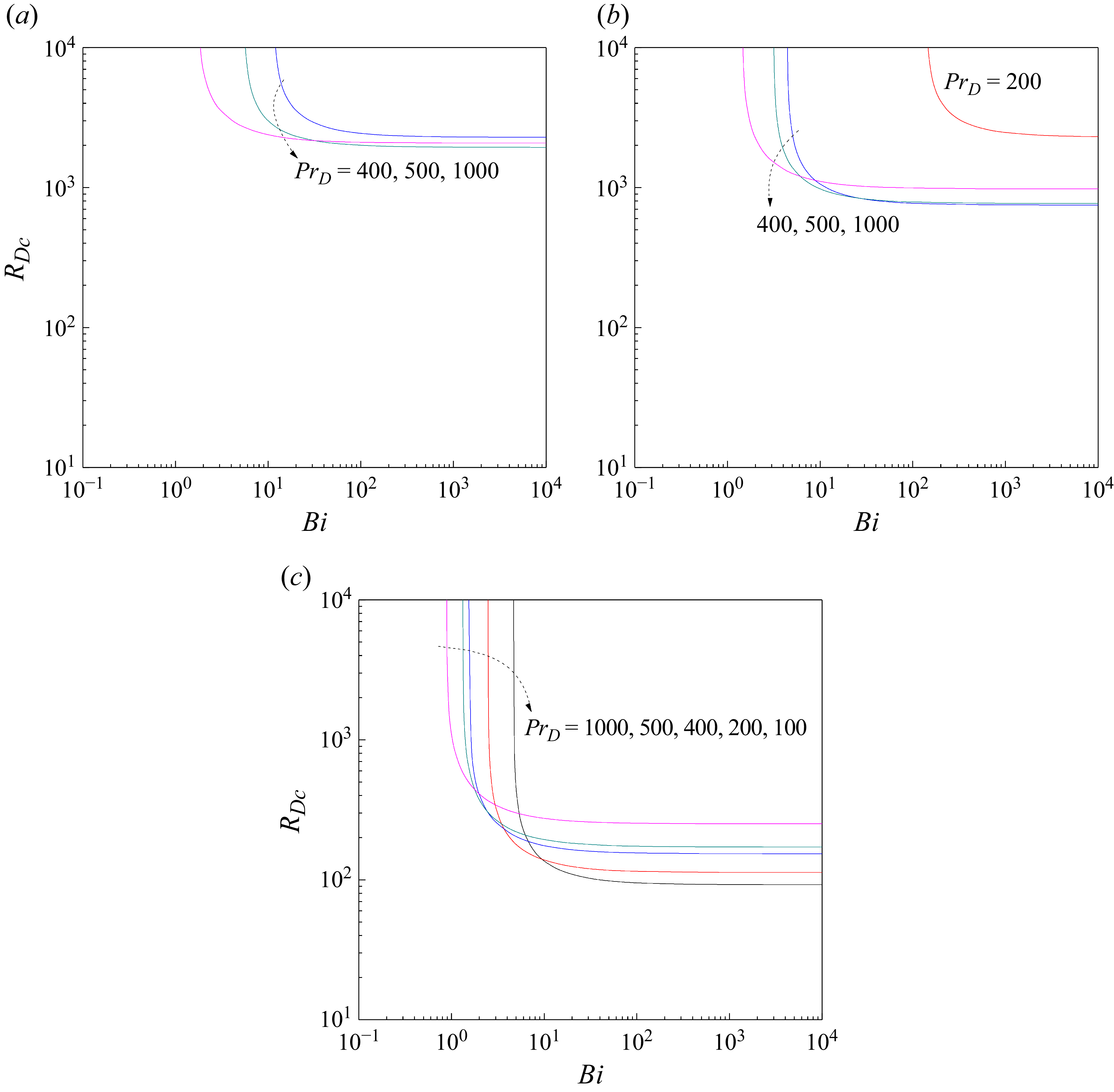
Critical value of
 $R_{D}$
versus
 ${\textit{Bi}}$
for (a)
 $\eta =0.5$
, (b)
 $\eta =1$
and (c)
 $\eta =1.5$
with different
 ${\textit{Pr}}_{D}$
.

6.2.1. Linear viscosity–temperature law
6.2.1.1. Linear stability boundaries.
The trends of
 $R_{\textit{Dc}}$
versus
 ${\textit{Bi}}$
for different values of
 ${\textit{Pr}}_{D}$
are displayed in figures 11(a), 11(b) and 11(c) where
 $\eta =0.5,1$
and
 $1.5$
, respectively. The results indicate that instability occurs only when
 ${\textit{Bi}}$
exceeds a finite threshold,
 $\tilde{B}i\gt 0$
, whose value depends sensitively on both
 ${\textit{Pr}}_{D}$
and
 $\eta$
. This behaviour differs sharply from the infinite-
 ${\textit{Pr}}_{D}$
limit (see § 6.1), where instability is altogether precluded for this form of viscosity variation. The finding that the system remains stable at
 $Bi=0$
is consistent with the observations of Shankar, Nagamani & Shivakumara (Reference Shankar, Nagamani and Shivakumara2023a
). To isolate the mechanism responsible for instability, we first consider the constant viscosity limit (figures not shown), where instability is found to arise only due to the combined action of finite
 ${\textit{Pr}}_{D}$
and
 ${\textit{Bi}}$
, since either acting alone remains stable. Instability is permitted for finite
 ${\textit{Pr}}_{D}$
because thermal perturbations remain long enough for buoyancy forces to act. In contrast, in the limit
 ${\textit{Pr}}_{D}\rightarrow \infty$
, temperature anomalies are smoothed out instantaneously, suppressing buoyancy and rendering the flow unconditionally stable. Similarly, when
 $Bi=0$
, perfectly isothermal walls absorb any thermal disturbance, preventing boundary-layer gradients and maintaining stability. As
 ${\textit{Bi}}$
increases, partial thermal resistance allows temperature gradients to develop near the boundaries, which, in conjunction with finite
 ${\textit{Pr}}_{D}$
, generate buoyancy forces that drive velocity perturbations and transport heat, thereby reinforcing the initial disturbances and sustaining the instability. Consequently, instability emerges for
 $Bi\gt 0$
and continues as
 $Bi\rightarrow \infty$
, where insulating boundaries further enhance boundary-layer temperature gradients. While viscosity stratification, characterised by the linear viscosity parameter
 $\eta \gt 0$
, is not required for this mechanism, it further destabilises the flow by reducing viscous damping near the hot wall, thereby lowering the critical threshold and amplifying the growth rate of perturbations. The role of
 ${\textit{Pr}}_{D}$
on base flow stability is conditional on
 ${\textit{Bi}}$
, as evidenced by the cross-over of
 $R_{\textit{Dc}}$
curves for different
 ${\textit{Pr}}_{D}$
with increasing
 ${\textit{Bi}}$
, thereby delineating regimes where
 ${\textit{Pr}}_{D}$
may stabilise, destabilise or exert a mixed influence on the flow. This behaviour arises because, at low
 $Bi , Pr_{D}$
tends to destabilise the flow, while at higher
 ${\textit{Bi}}$
its role is modified, leading to a shift in the dominant mechanism. This trend is maintained across all values of
 $\eta$
considered (figure 11
a–c). Notably, each figure considers distinct sets of
 ${\textit{Pr}}_{D}$
values for different
 $\eta$
indicate that instability is confined to restricted
 ${\textit{Pr}}_{D}$
ranges, which shift systematically to lower values as
 $\eta$
increases. It is also observed from the figures that
 $R_{\textit{Dc}}$
decreases monotonically with increasing
 ${\textit{Bi}}$
and approaches an asymptotic value as
 $Bi\rightarrow \infty$
for all considered values of
 ${\textit{Pr}}_{D}$
and
 $\eta$
. Physically, this reflects that insulating boundaries suppress thermal leakage into the surroundings, thereby allowing weaker external heating to induce instability more readily than in the partially conducting case.
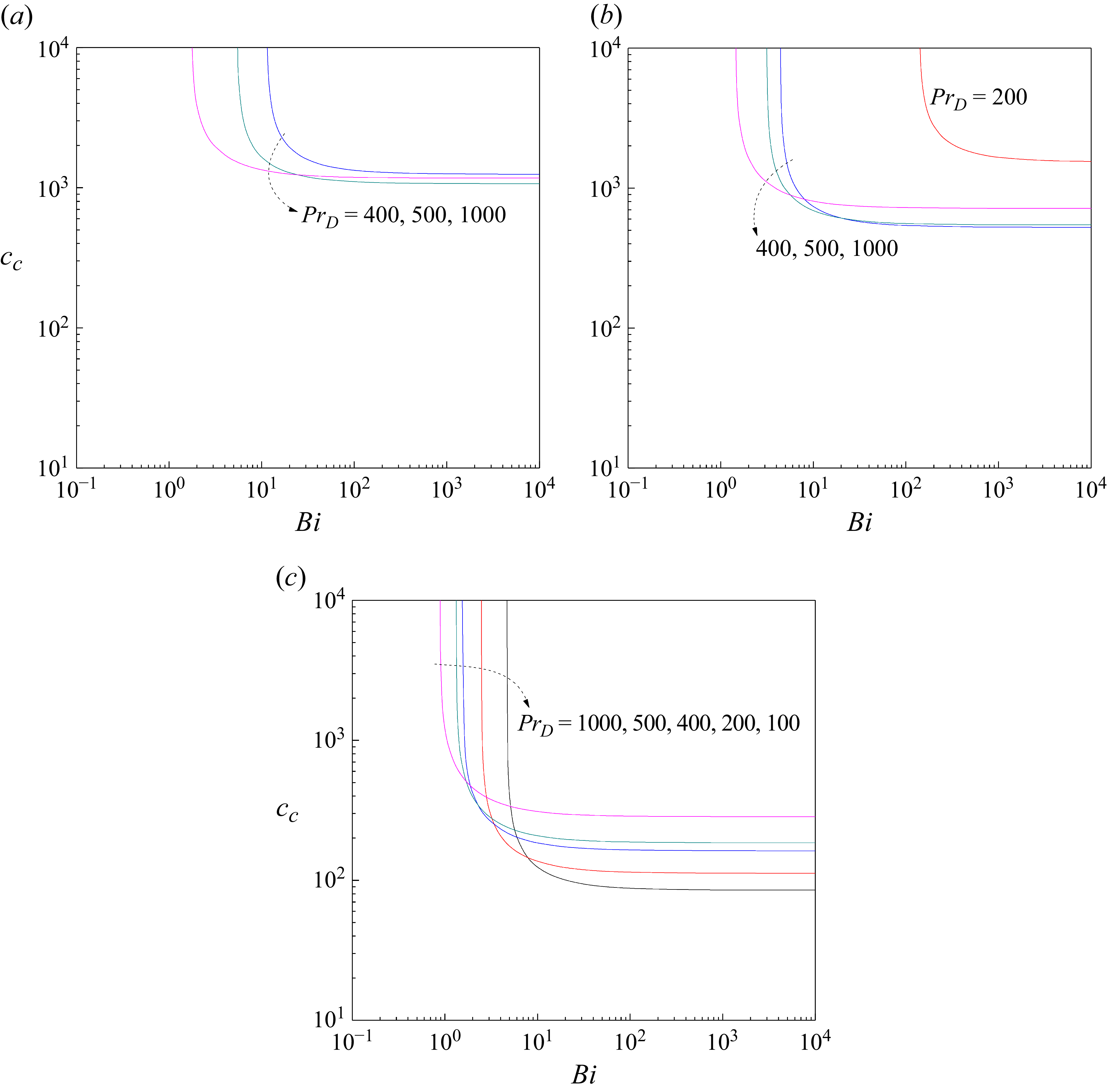
The corresponding variations of the critical wavenumber
 $a_{c}$
and critical wave speed
 $c_{c}$
are presented in figures 12(a–c) and 13(a–c), respectively. It is seen that
 $a_{c}$
increases steeply at small
 ${\textit{Bi}}$
before saturating to a weak
 ${\textit{Bi}}$
-dependence at larger values, a trend that is consistent across all
 ${\textit{Pr}}_{D}$
and
 $\eta$
. Increasing either
 ${\textit{Pr}}_{D}$
or
 $\eta$
leads to larger
 $a_{c}$
, signifying that the convection cells become progressively narrower as viscous resistance or viscosity stratification strengthens (figure 12
a–c). The critical wave speed
 $c_{c}$
remains strictly positive throughout the parameter space, confirming that the unstable modes propagate upward (figure 13
a–c). Moreover, the qualitative form of the
 $c_{c}$
curves closely parallel that of the
 $R_{\textit{Dc}}$
curves, highlighting the intrinsic link between the onset of instability and the associated travelling-wave behaviour.
Critical value of
 $a$
versus
 ${\textit{Bi}}$
for (a)
 $\eta =0.5$
, (b)
 $\eta =1$
and (c)
 $\eta =1.5$
with different
 ${\textit{Pr}}_{D}$
.

Critical value of
 $c$
versus
 ${\textit{Bi}}$
for (a)
 $\eta =0.5$
, (b)
 $\eta =1$
and (c)
 $\eta =1.5$
with different
 ${\textit{Pr}}_{D}$
.

6.2.1.2. Stability and instability zone.
The asymptotic behaviour, characterised by
 $R_{\textit{Dc}}\rightarrow \infty$
and
 $a_{c}\rightarrow 0$
as
 $Bi\rightarrow \tilde{B}i\gt 0$
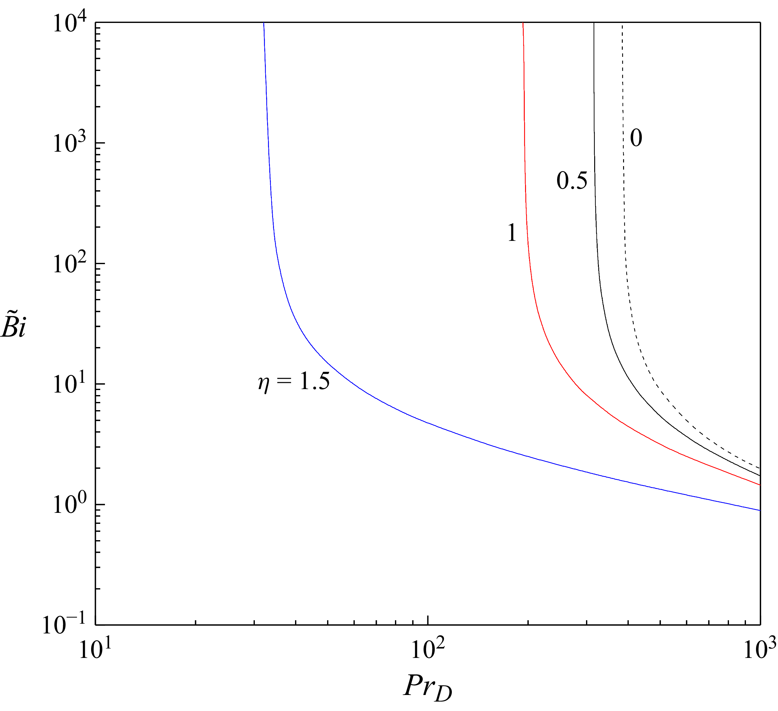
, evident in figures 11 and 12, is further substantiated in figure 14, which depicts the transition curves delineating the stability boundary in the
 $(Pr_{D},\tilde{B}i)$
-plane for different
 $\eta$
. The region above each curve corresponds to instability, while the region below denotes stability. Instability, manifested by the emergence of
 $\tilde{B}i$
, appears only beyond a certain value of
 ${\textit{Pr}}_{D}$
, and this threshold shifts progressively to lower values as
 $\eta$
increases. The curves further show a systematic decrease of
 $\tilde{B}i$
with increasing
 ${\textit{Pr}}_{D}$
and
 $\eta$
.
Stability and instability zones in the (
 ${\textit{Pr}}_{D},\,\tilde{B}i$
)-plane for different
 $\eta$
. The region beneath each curve corresponds to stability, whereas instability arises along and above the curves.

6.2.1.3. Streamlines and isotherms.
Figures 15(a) and 15(b) display the streamlines and isotherms, respectively, at the onset of instability for
 ${\textit{Pr}}_{D}=200 , Bi=140$
and
 $\eta =1$
. The streamlines are denser near the hot wall, with elongated structures extending toward the cold wall, while the corresponding isotherms form open cells adjacent to the hot boundary that protrude into the external region (
 $x\gt 1$
). Variations in
 $Bi , Pr_{D}$
and
 $\eta$
do not modify the secondary-flow pattern in any essential way, apart from a slight rightward displacement of the structure with increasing
 ${\textit{Pr}}_{D}$
. Since this shift is marginal and the overall topology remains preserved, the single representative case shown here captures the key flow features with full clarity, rendering additional illustrations unnecessary.
(a) Streamlines and (b) isotherms of the perturbation modes at the onset of instability for
 $\eta =1,Pr_{D}=200$
and
 $Bi=140$
at a fixed
 $t$
.

6.2.2. Quadratic viscosity–temperature law
6.2.2.1. Linear stability boundaries.
The variation of the critical stability parameters with
 ${\textit{Bi}}$
for different
 ${\textit{Pr}}_{D}$
is illustrated in figures 16–18, where figure 16 shows
 $R_{\textit{Dc}}$
, figure 17
 $a_{c}$
and figure 18
 $| c_{c}|$
. In each figure, panels (a), (b) and (c) correspond to
 $\Gamma =1 , 2$
and
 $3$
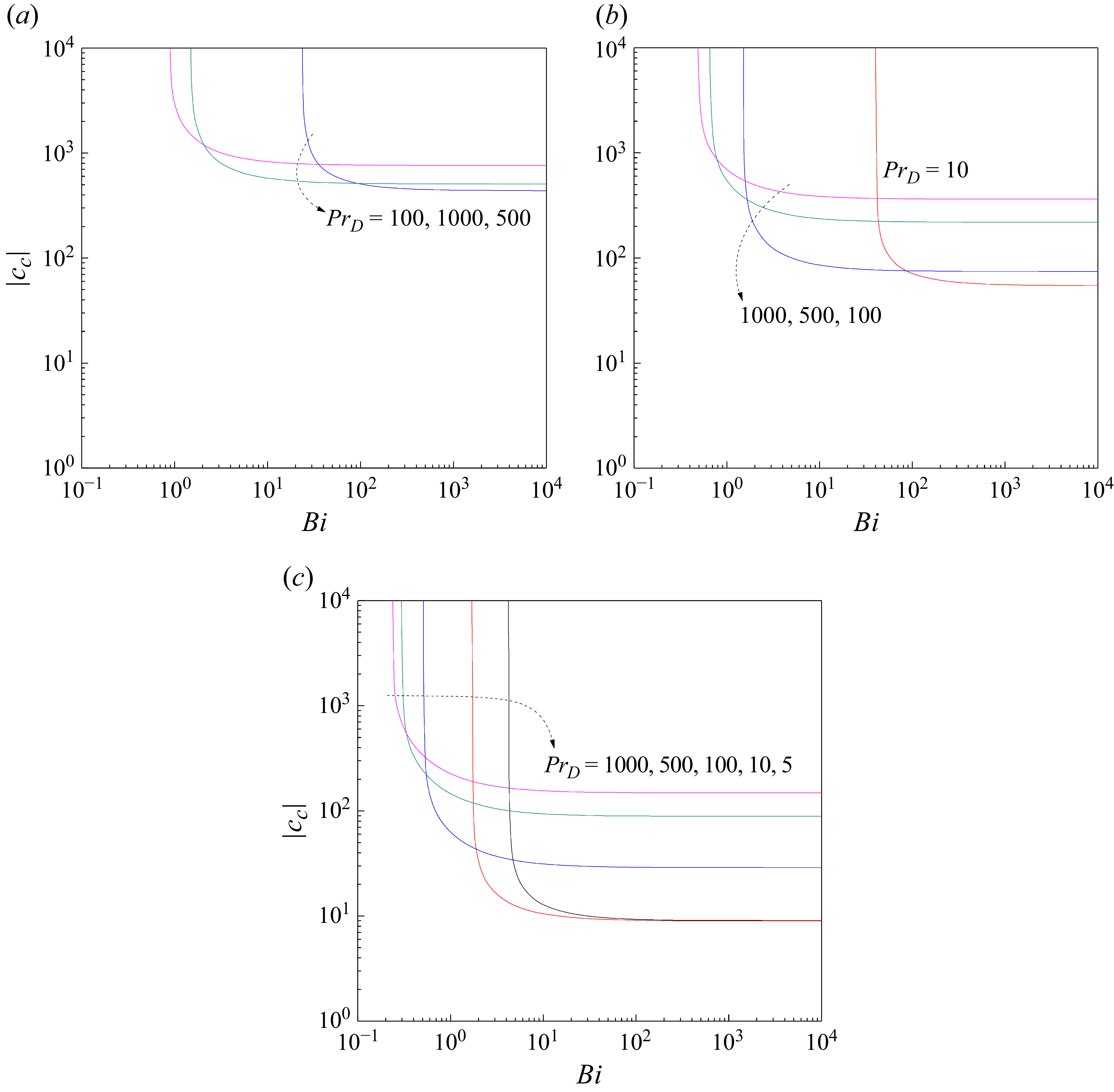
, respectively. A key outcome is that the quadratic viscosity–temperature law also admits the occurrence of instability, in complete analogy with the linear law. This result stands in sharp contrast to earlier findings, where instability was ruled out either in the infinite-
 ${\textit{Pr}}_{D}$
limit (see § 6.1) or under perfectly conducting boundaries (
 $Bi=0$
; Shankar, Nagamani & Shivakumara Reference Shankar, Nagamani and Shivakumara2023b
). Since the overall behaviour mirrors the linear case, a detailed repetition of the discussion is therefore not required. The essential trends are summarised as follows. For fixed
 $\Gamma$
, the curves of
 $R_{\textit{Dc}}$
for different
 ${\textit{Pr}}_{D}$
exhibit a cross-over with increasing
 ${\textit{Bi}}$
, while
 $R_{\textit{Dc}}$
decreases monotonically as both
 $\Gamma$
and
 ${\textit{Bi}}$
increase (figure 16). The critical wavenumber
 $a_{c}$
increases systematically with
 ${\textit{Pr}}_{D}$
,
 ${\textit{Bi}}$
and
 $\Gamma$
(figure 17), and the phase speed
 $| c_{c}|$
closely tracks the variation of
 $R_{\textit{Dc}}$
(figure 18). A closer comparison between the linear case (
 $\eta =1$
) and the quadratic case (
 $\Gamma =1$
) highlights three salient distinctions: (i) instability sets in at lower
 $R_{\textit{Dc}}$
under the quadratic law than under the linear one, although this trend reverses as
 ${\textit{Bi}}$
increases, (ii) the convection cells are larger for the linear law, as evidenced by the smaller critical wavenumber and (iii) under the quadratic relation,
 $c_{c}$
assumes equal and opposite values, indicating that the unstable mode propagates upward and downward with the same speed, whereas in the linear law it travels only upward.
Critical value of
 $R_{D}$
versus
 ${\textit{Bi}}$
for (a)
 $\Gamma =1$
, (b)
 $\Gamma =2$
and (c)
 $\Gamma =3$
with different
 ${\textit{Pr}}_{D}$
.

Critical value of
 $a$
versus
 ${\textit{Bi}}$
for (a)
 $\Gamma =1$
, (b)
 $\Gamma =2$
and (c)
 $\Gamma =3$
with different
 ${\textit{Pr}}_{D}$
.

Critical value of
 $|c|$
versus
 ${\textit{Bi}}$
for (a)
 $\Gamma =1$
, (b)
 $\Gamma =2$
and (c)
 $\Gamma =3$
with different
 ${\textit{Pr}}_{D}$
.

6.2.2.2. Stability and instability zone.
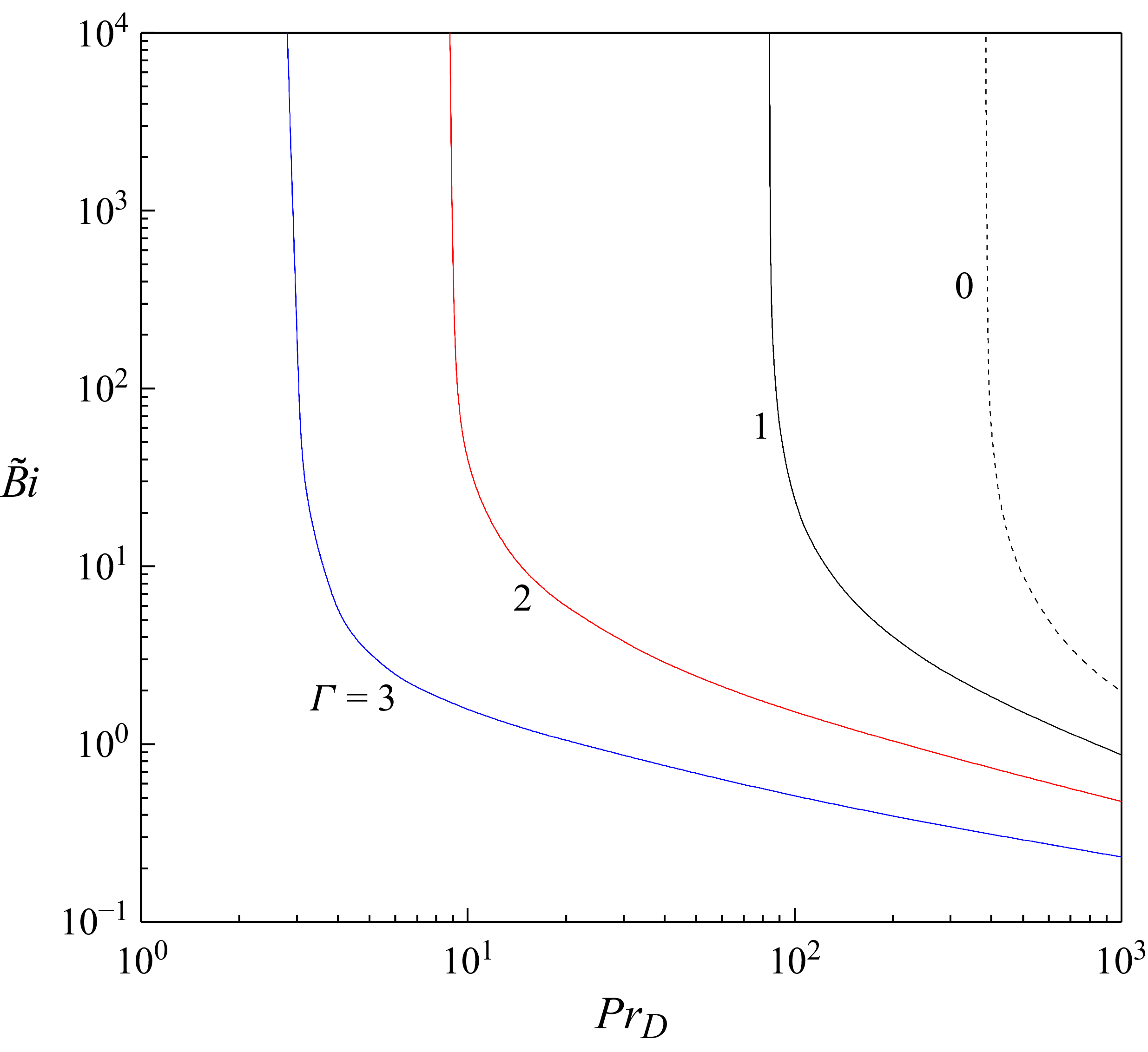
The regions of stability and instability, delineated by the stability boundaries in the
 $(Pr_{D},\tilde{B}i)$
-plane, shown in figure 19, reveal that
 $\tilde{B}i$
decreases consistently with both
 ${\textit{Pr}}_{D}$
and
 $\Gamma$
, and emerges only beyond a finite threshold of
 ${\textit{Pr}}_{D}$
that itself decreases as
 $\Gamma$
increases. Moreover, the quadratic viscosity law induces instability at lower
 ${\textit{Pr}}_{D}$
than the linear counterpart. In addition, the
 $\tilde{B}i$
values in this plane associated with the quadratic law lie substantially below those of the linear case.
Stability and instability zones in the (
 ${\textit{Pr}}_{D},\,\tilde{B}i$
)-plane for different
 $\Gamma$
. The region beneath each curve corresponds to stability, whereas instability arises along and above the curves.

6.2.2.3. Streamlines and isotherms.
The secondary-flow patterns are presented for
 ${\textit{Pr}}_{D}=5$
(figure 20) and
 ${\textit{Pr}}_{D}=1000$
(figure 21) with
 $\Gamma =3$
and
 $Bi=25$
. The lower value
 ${\textit{Pr}}_{D}=5$
is chosen because the order-unity case is of particular interest, and in this
 ${\textit{Pr}}_{D}$
-regime the linear law remains stable. At
 ${\textit{Pr}}_{D}=5$
, the streamlines extend across the layer but are concentrated near the hot wall, while the isotherms form a truncated cell adjacent to the hot wall that stretches toward the cold wall. At large
 ${\textit{Pr}}_{D}$
(figure 21), the disturbance fields are essentially identical to those of the linear law. Variations in
 ${\textit{Bi}}$
and
 $\Gamma$
do not produce any qualitative alteration in these patterns (figures not shown).
(a) Streamlines and (b) isotherms of the perturbation modes at the onset of instability for
 $\Gamma =3,Pr_{D}=5$
and
 $Bi=25$
at a fixed
 $t$
.

(a) Streamlines and (b) isotherms of the perturbation modes at the onset of instability for
 $\Gamma =3,Pr_{D}=10^{3}$
and
 $Bi=25$
at a fixed
 $t$
.

6.2.3. Exponential viscosity–temperature law
6.2.3.1. Linear stability boundaries.
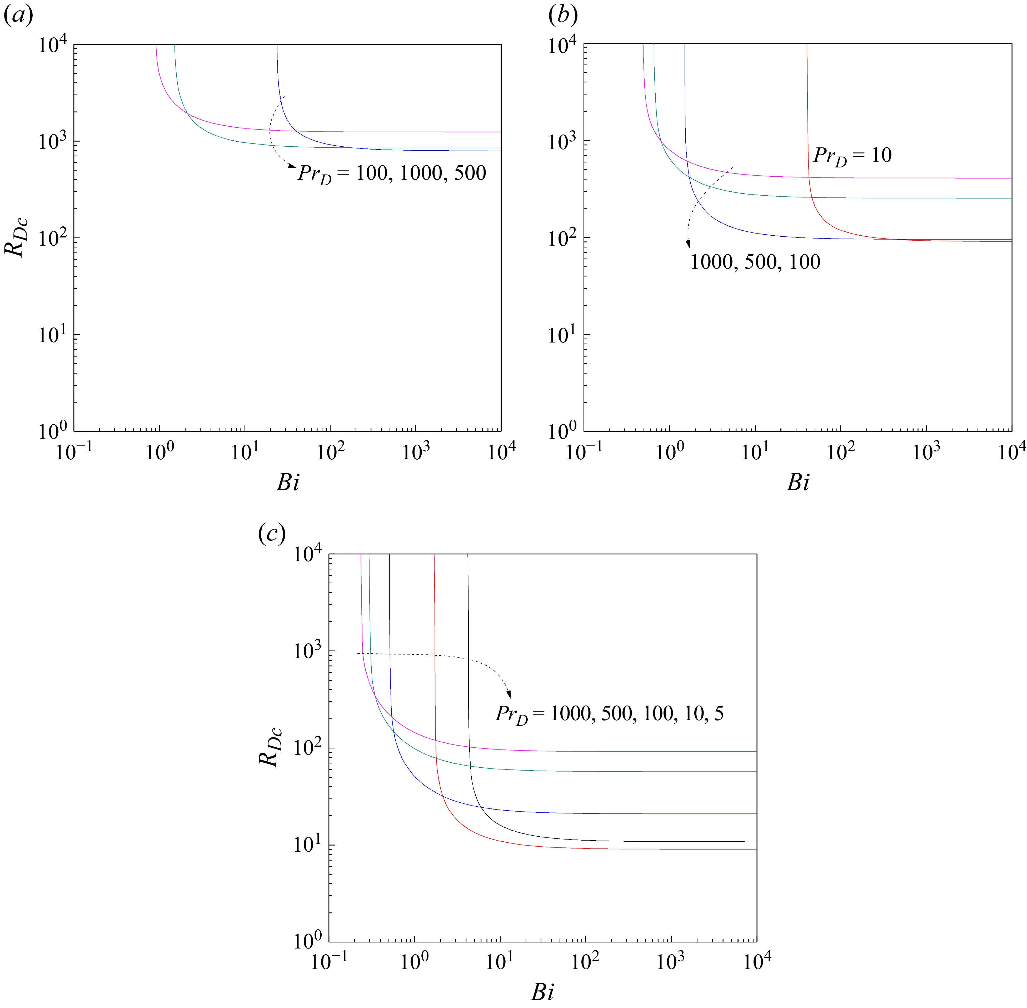
Figure 22(a–c) depicts the dependence of
 $R_{\textit{Dc}}$
on
 ${\textit{Bi}}$
for different values of
 ${\textit{Pr}}_{D}$
, with each panel corresponding to a fixed
 $\Upsilon$
: (a)
 $\Upsilon=5$
, (b)
 $\Upsilon=10$
and (c)
 $\Upsilon=15$
. Although instability persists in the asymptotic limit
 ${\textit{Pr}}_{D}\rightarrow \infty$
, introducing a finite
 ${\textit{Pr}}_{D}$
fundamentally alters the stability landscape. In particular, for finite
 ${\textit{Pr}}_{D}$
, instability becomes active beyond a certain
 $Bi\gt 0$
and, when
 $\Upsilon$
is sufficiently large, may even occur at
 $Bi=0$
; it then extends continuously up to
 $Bi\rightarrow \infty$
, corresponding to adiabatic boundaries. By contrast, for
 ${\textit{Pr}}_{D}\rightarrow \infty$
, instability occurs only within a bounded interval of
 ${\textit{Bi}}$
(see § 6.1). For
 $\Upsilon=5$
, figure 22(a) shows that instability is restricted to a relatively narrow range of
 ${\textit{Pr}}_{D}$
, within which increasing
 ${\textit{Pr}}_{D}$
exerts a distinctly stabilising influence. For
 $\Upsilon=10$
(figure 22
b), the behaviour changes markedly. New phenomena appear that are absent under either the linear or quadratic viscosity laws, and even under the exponential law of Model I. In this case,
 $R_{\textit{Dc}}$
decreases with
 ${\textit{Bi}}$
, but at sufficiently small
 ${\textit{Pr}}_{D}$
a sharp drop occurs at a certain
 ${\textit{Bi}}$
where a cusp forms, signalling a transition between two competing instability modes. At the cusp point, the
 $R_{\textit{Dc}}$
curves bifurcate into two distinct branches. The dotted segments denote formal continuations that do not correspond to the most unstable modes and are therefore irrelevant to the onset of instability. Before the cusp, increasing
 ${\textit{Pr}}_{D}$
has a stabilising influence, whereas beyond it the behaviour becomes non-uniform, with the curves for different
 ${\textit{Pr}}_{D}$
crossing as
 ${\textit{Bi}}$
increases. At larger
 ${\textit{Pr}}_{D}$
the cusp disappears, restoring a smoother trend. In the limit
 $Bi\rightarrow \infty$
, the stabilising influence of increasing
 ${\textit{Pr}}_{D}$
is ultimately recovered. For
 $\Upsilon=15$
(figure 22
c), the stability characteristics change even more dramatically. Instability now occurs in two distinct windows of
 ${\textit{Bi}}$
, separated by a finite interval of stability. The first, novel regime extends from
 $Bi=0$
, where
 $R_{\textit{Dc}}$
exhibits a striking departure from monotonic trend: it decreases slightly before rising sharply with
 ${\textit{Bi}}$
. This sequence of destabilisation followed by stabilisation is highly counterintuitive, with no analogue either under alternative viscosity laws or within the steady Darcy framework. In this regime, increasing
 ${\textit{Pr}}_{D}$
has only a negligible stabilising effect. The
 $R_{\textit{Dc}}$
curve terminates at a finite
 ${\textit{Bi}}$
, beyond which the system remains stable over a bounded interval of
 ${\textit{Bi}}$
, as the growth rate remains negative throughout. Instability re-emerges with further increase in
 ${\textit{Bi}}$
, marking the onset of the second regime. Here, two competing modes coexist, reminiscent of the behaviour at
 $\Upsilon=10$
for small
 ${\textit{Pr}}_{D}$
, but unlike that case the mode competition persists even at higher
 ${\textit{Pr}}_{D}(=100)$
. To avoid visual clutter, extensions of
 $R_{\textit{Dc}}$
beyond the discontinuities are omitted in figure 22(c), since the abrupt breaks already expose the transitions between dominant modes. A complementary examination of
 $R_{\textit{Dc}}$
as a function of
 ${\textit{Bi}}$
for different values of
 $\Upsilon$
for a fixed
 ${\textit{Pr}}_{D}$
(figures not shown) provides additional insight into the role of
 $\Upsilon$
. For small
 ${\textit{Pr}}_{D}$
, the curves of
 $R_{\textit{Dc}}$
corresponding to different
 $\Upsilon$
intersect as
 ${\textit{Bi}}$
increases, revealing a delicate balance between the effects of thermal boundary conditions and viscosity variations. In contrast, at large
 ${\textit{Pr}}_{D}$
, the influence of
 $\Upsilon$
becomes unambiguous: increasing
 $\Upsilon$
consistently destabilises the flow.
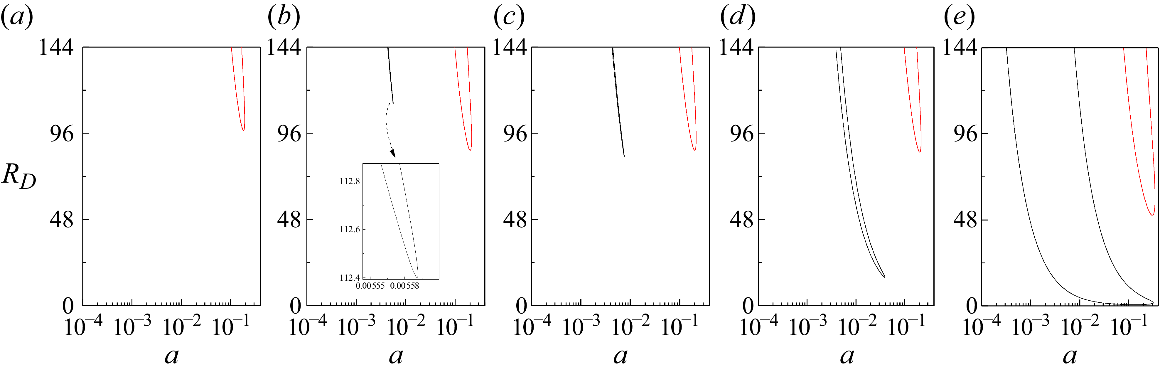
To elucidate the transition in the mode of instability observed in figure 22(b), the evolution of the neutral curves near the cusp point is shown for
 ${\textit{Pr}}_{D}=10$
in figure 23. At
 $Bi=7$
(figure 23
a), a single neutral curve exists, corresponding to a mode with
 $c_{c}\gt 0$
. At
 $Bi=7.882$
(figure 23
b), this curve undergoes a qualitative change as two distinct neutral branches emerge, each associated with a different eigenmode, both characterised by
 $c_{c}\gt 0$
. For clarity, the left branch is designated as the lower-wavenumber branch and the right as the higher-wavenumber branch. Despite both branches coexist, the instability is governed by the higher-wavenumber mode. At
 $Bi=7.884$
(figure 23
c), however, the lower-wavenumber branch deepens significantly and overtakes its counterpart, thereby becoming the preferred mode of instability. With further increase in
 ${\textit{Bi}}$
, the lower-wavenumber mode continues to dominate, although both branches persist (figures 23
d and 23
e). Thus, figure 23 demonstrates that the cusp in figure 22(b) corresponds to a switch in the dominant mode of instability from the higher- to the lower-wavenumber mode, whereas at larger
 ${\textit{Pr}}_{D}$
this switch does not occur, the instability being governed by a single wavenumber mode.
Critical value of
 $R_{D}$
versus
 ${\textit{Bi}}$
for (a)
 $\Upsilon=5$
, (b)
 $\Upsilon=10$
and (c)
 $\Upsilon=15$
with different
 ${\textit{Pr}}_{D}$
.

Evolution of neutral stability curves for (a)
 $Bi=7$
, (b)
 $Bi=7.882$
, (c)
 $Bi=7.884$
, (d)
 $Bi=8$
and (e)
 $Bi=100$
with
 $\Upsilon=10$
and
 ${\textit{Pr}}_{D}=10$
.

The variations of
 $a_{c}$
and
 $c_{c}$
, corresponding to those of
 $R_{\textit{Dc}}$
in figure 22, are displayed in figures 24 and 25, respectively, with vertical lines indicating discontinuities associated with transitions between distinct instability modes. For
 $\Upsilon=5$
(figure 24
a),
 $a_{c}$
exhibits a mixed trend: it rises with increasing
 ${\textit{Bi}}$
, reaches a maximum, and then decreases with further increase in
 ${\textit{Bi}}$
. A comparable pattern is observed for
 $\Upsilon=10$
(figure 24
b), but only after the mode transition, where the instability is governed by the low-wavenumber branch. In the pre-transition range, by contrast,
 $a_{c}$
increases with
 ${\textit{Bi}}$
. At higher
 ${\textit{Pr}}_{D}$
, where no transition occurs,
 $a_{c}$
simply grows with
 ${\textit{Bi}}$
and gradually approaches an asymptotic value. For
 $\Upsilon=15$
(figure 24
c), in the first instability regime,
 $a_{c}$
increases marginally before dropping sharply with
 ${\textit{Bi}}$
, while in the second regime its variation closely resembles the behaviour observed for
 $\Upsilon=10$
. Moreover, although
 $a_{c}$
decreases with
 ${\textit{Pr}}_{D}$
prior to the mode transition, its subsequent variation becomes non-uniform, reflecting a delicate interplay between
 ${\textit{Bi}}$
and
 $\Upsilon$
. Despite the complexity of these transitions and the emergence of dual
 ${\textit{Bi}}$
-regimes at higher
 $\Upsilon$
, the direction of propagation of unstable modes remains unaffected: they travel unidirectionally along the positive
 $z$
-direction, as confirmed by the consistently positive values of
 $c_{c}$
(figure 25
a–c).
Critical value of
 $a$
versus
 ${\textit{Bi}}$
for (a)
 $\Upsilon=5$
, (b)
 $\Upsilon=10$
and (c)
 $\Upsilon=15$
with different
 ${\textit{Pr}}_{D}$
.

Critical value of
 $c$
versus
 ${\textit{Bi}}$
for (a)
 $\Upsilon=5$
, (b)
 $\Upsilon=10$
and (c)
 $\Upsilon=15$
with different
 ${\textit{Pr}}_{D}$
.

6.2.3.2. Stability and instability zone.
The bifurcation values
 $\tilde{B}i$
, marking the transition between stable and unstable states, is mapped in the
 $(Pr_{D},\tilde{B}i)$
-plane in figure 26(a–c) for three representative values of
 $\Upsilon$
. For
 $\Upsilon=5$
(figure 26
a), the bifurcation curve increases with
 ${\textit{Pr}}_{D}$
and blows up at a finite
 ${\textit{Pr}}_{D}$
, beyond which the system remains unconditionally stable. In contrast, for
 $\Upsilon=10$
(figure 26
b) and
 $15$
(figure 26
c), no finite-
 ${\textit{Pr}}_{D}$
cutoff appears, and instability prevails irrespective of how large
 ${\textit{Pr}}_{D}$
becomes. For
 $\Upsilon=10$
, curve A separates stability beneath it from instability at and above, while curve B, situated entirely within the unstable domain, serves as an internal divider: the region between A (inclusive) and B corresponds to instabilities governed by higher-wavenumber modes, whereas at and above B lower-wavenumber disturbances dominate. The two curves evolve in strikingly different ways with
 ${\textit{Pr}}_{D}$
: curve A increases gradually, delaying the onset of instability, while curve B follows a more intricate trajectory – decreasing initially, then rising steeply and finally culminating at a finite
 ${\textit{Pr}}_{D}$
with
 $\tilde{B}i\rightarrow \infty$
. For
 $\Upsilon=15$
, the bifurcation structure is markedly more complex, comprising four distinct branches (A–D). The first instability regime, extending up to and including curve C, is internally partitioned by curve D: below D, the system exhibits a destabilising trend (
 $R_{\textit{Dc}}$
decreases with increasing
 ${\textit{Bi}}$
, see figure 22
c), whereas the region from D to C corresponds to a stabilising effect. Both curves C and D shift downward with increasing
 ${\textit{Pr}}_{D}$
and eventually approach one another closely where
 $\tilde{B}i$
is very small (approaching zero). Beyond curve C, a stable region emerges and extends up to curve A. Curve A then signals the onset of a second instability window, which itself is divided into two subdomains: from A up to but not including B, instability is dominated by higher-wavenumber disturbances, while from B onwards the dynamics is governed by lower-wavenumber modes, terminating at a finite
 ${\textit{Pr}}_{D}$
in close analogy with the
 $\Upsilon=10$
case.
Stable and unstable zones in the (
 ${\textit{Pr}}_{D},\,\tilde{B}i$
)-plane for (a)
 $\Upsilon=5$
, (b)
 $\Upsilon=10$
and (c)
 $\Upsilon=15$
.

6.2.3.3. Streamlines and isotherms.
Streamlines and isotherms are provided to visualise the reorganisation of the flow at the mode transition and to quantify its deviation from the infinite-
 ${\textit{Pr}}_{D}$
limit. We focus first on the case
 ${\textit{Pr}}_{D}=10$
and
 $\Upsilon=10$
, with
 ${\textit{Bi}}$
chosen close to the transition where the dominant instability shifts from the higher- to the lower-wavenumber branch (figure 27). For
 $Bi=5$
(figures 27
a and 27
e) and
 $Bi=7.883$
(figures 27
b and 27
f), the flow closely resembles the infinite-
 ${\textit{Pr}}_{D}$
limit: streamlines remain confined to the hot wall, while the isotherms, anchored at the same boundary, extend progressively across the layer toward the cold wall, remaining open near that side. This configuration is characteristic of the higher-wavenumber branch. A qualitative change occurs at
 $Bi=7.884$
(figures 27
c and 27
g), where the streamlines acquire a slight vertical tilt and become compressed against the hot boundary, indicating a restructuring of the modal organisation. The corresponding isotherms no longer form closed cell-like structures but instead evolve into nearly horizontal layers with gentle undulations that deflect toward the side boundaries, signalling the transition to the lower-wavenumber branch. In the adiabatic limit (
 $Bi\rightarrow \infty$
, figures 27
d and 27
h), the streamlines retain their wall-attached character, although with reduced tilt and intensified clustering along the hot boundary, while the isotherms collapse into almost perfectly horizontal bands, consistent with perturbations sustained by an essentially vanishing transverse temperature gradient. For
 $\Upsilon=15$
, two distinct regimes of
 ${\textit{Bi}}$
are identified (figure 22
c). The second regime closely resembles that for
 $\Upsilon=10$
, including the secondary-flow patterns, and is therefore omitted for brevity. Attention is instead confined to the first regime, which is unique to
 $\Upsilon=15$
. Within this regime, increasing
 ${\textit{Bi}}$
leaves the overall streamline topology remains broadly similar to that observed elsewhere, with recirculations confined to the vicinity of the heated boundary (figure 28
a–d). The isotherms are elongated from the hot wall toward the cold wall (figure 28
e–h). Notably, unlike in the second regime, where thermal cells preferentially extend horizontally, the present regime exhibits vertically oriented cells, signalling a fundamental reorientation of the convective transport and a qualitatively different mechanism of instability. Variation in
 ${\textit{Pr}}_{D}$
does not substantially modify the secondary-flow (figures not shown).
Streamlines (a–d) and isotherms (e–h) of the perturbation modes at the onset of instability
 $\Upsilon=10$
and
 ${\textit{Pr}}_{D}=10$
with different
 ${\textit{Bi}}$
at a fixed
 $t$
.

Streamlines (a–d) and isotherms (e–h) of the perturbation modes at the onset of instability for
 $\Upsilon=15$
and
 ${\textit{Pr}}_{D}=10$
with different
 ${\textit{Bi}}$
at a fixed
 $t$
.

7. Conclusions
The linear stability of natural convection in a vertical porous slab saturated with a fluid of variable viscosity and bounded by imperfectly conducting walls is analysed. The analysis considered three representative viscosity–temperature relations: linear, quadratic and exponential. The flow through porous media is governed by the modified Darcy law. The thermal exchange at the boundaries is characterised by the Biot number
 ${\textit{Bi}}$
, spanning the limits from isothermal (
 $Bi=0$
) to adiabatic (
 $Bi\rightarrow \infty$
), with finite
 ${\textit{Bi}}$
representing partial heat transfer. The stability characteristics are governed by the Darcy–Rayleigh number
 $R_{D}$
, Biot number
 ${\textit{Bi}}$
, the parameters
 $\eta ,\,\Gamma$
and
 $\Upsilon$
associated with linear, quadratic and exponential form of viscosity variations, respectively, and the Prandtl–Darcy number,
 ${\textit{Pr}}_{D}$
, encompassing the asymptotic limit
 ${\textit{Pr}}_{D}\rightarrow \infty$
(Model I) and finite
 ${\textit{Pr}}_{D}$
(Model II). The numerical solution of the resulting eigenvalue problem yields the neutral stability condition and the critical value of
 $R_{D}$
, thereby delineating the onset of convective instability for different values of governing parameters.
The principal outcomes of our analysis for Model I and Model II may be summarised as follows:
Model I
-
(i) For linear and quadratic variations of viscosity with temperature, the base flow remains unconditionally stable to infinitesimal disturbances, irrespective of the nature of thermal boundary conditions.
-
(ii) The exponential dependence of viscosity on temperature assures instability of the base flow, but only within a finite interval of
 ${\textit{Bi}}$
, whose width increases with
$\Upsilon$
.
-
(iii) The system remains stable for
$\Upsilon\lt 8.2070$
, independent of thermal boundary conditions. -
(iv) The onset of instability is hastened with increasing
${\textit{Bi}}$
and
$\Upsilon$
, accompanied by a reduction in the size of the convection cells. -
(v) The instability manifests exclusively through travelling-wave modes, propagating upward at low
${\textit{Bi}}$
for all values of
$\Upsilon$
. At high
${\textit{Bi}}$
, however, the propagation direction reverses from downward to upward with increasing
$\Upsilon$
.


Model II
-
(i) For all three viscosity–temperature relationships, instability arises under imperfectly conducting boundaries through travelling-wave modes and persists up to the adiabatic limit
$Bi\rightarrow \infty$
, and the onset occurring earlier for adiabatic boundaries. -
(ii) For both linear and quadratic viscosity variations, instability arises only through the combined action of Biot number and a finite Prandtl–Darcy number. The threshold Biot number at which instability sets in decreases with increasing
${\textit{Pr}}_{D}$
and viscosity parameter (
$\eta /\Gamma$
). The range of
${\textit{Pr}}_{D}$
over which instability exists broadens as
$\eta /\Gamma$
increases. While
${\textit{Bi}}$
and the viscosity parameters invariably act to destabilise the system,
${\textit{Pr}}_{D}$
exerts a non-monotonic influence on the base flow, governed by its interplay with other controlling parameters. The characteristic cell width of the unstable mode decreases with increasing
$Bi , Pr_{D}$
and
$\eta /\Gamma$
. The travelling-wave mode propagates exclusively upward for the linear viscosity–temperature law, but in both directions with equal speed for the quadratic law. -
(iii) The exponential viscosity law departs sharply from its linear and quadratic counterparts. For small values of
$\Upsilon$
, instability emerges only beyond a threshold in
${\textit{Bi}}$
and within a narrow interval of
${\textit{Pr}}_{D}$
. At intermediate
$\Upsilon$
, instability appears above a threshold
${\textit{Bi}}$
, accompanied by a mode transition at a specific
${\textit{Bi}}$
where the dominant instability mode shifts from higher to lower wavenumber; this transition gradually disappears as
${\textit{Pr}}_{D}$
increases. For larger
$\Upsilon$
, a similar mode-transition trend persists, and an additional instability regime develops, yielding two distinct
${\textit{Bi}}$
-instability regimes separated by a stability window. The first of these regimes, commencing at
$Bi=0$
, exhibits the unusual sequence of an initial destabilisation followed by stabilisation as
${\textit{Bi}}$
increases, before the instability ceases at a finite
${\textit{Bi}}$
. Besides,
$Bi , Pr_{D}$
and
$\Upsilon$
act in strong interdependence, exerting a contrasting influence on both instability onset and cell width, while the travelling cells always propagate upward.


Several avenues for future investigation remain open. Foremost among them is the investigation of threshold conditions governing the onset of absolute instability. Another natural extension is the exploration of the supercritical regime, where the mechanisms of nonlinear saturation may be probed either through weakly nonlinear theory or fully nonlinear numerical simulation. Such approaches would also enable an assessment of the possible existence of subcritical bifurcations. In this context, the energy method provides a valuable complementary framework for analysing the response of the system to finite-amplitude disturbances and for elucidating the dynamics beyond the linear threshold.
Acknowledgements
The authors gratefully acknowledge the referees for their incisive and constructive comments, which have significantly enhanced the clarity and quality of this work.
Declaration of interests
The authors have no conflicts to disclose.
Data availability
The data that support the findings of this study are available within the article.