


Introduction
Posidonia oceanica (L.) Delile, 1813 meadows are key ecosystems of the Mediterranean Sea (Boudouresque et al., Reference Boudouresque, Bernard, Bonhomme, Charbonnel, Le Dieréach and Ruitton2007). These underwater seagrasses are well known for their multiple and diverse ecosystem services, including coastal protection from erosion (Sánchez-González et al., Reference Sánchez-González, Sánchez-Rojas and Memos2011), stabilization of the seabed (Terrados and Duarte, Reference Terrados and Duarte2000; Gacia and Duarte, Reference Gacia and Duarte2001), and oxygen production (Agueda Aramburu et al., Reference Agueda Aramburu, Flecha, Lujan-Williams and Hendriks2024). They also serve as important nurseries and breeding habitats for many animal species (Boudouresque et al., Reference Boudouresque, Bernard, Bonhomme, Charbonnel, Le Dieréach and Ruitton2007; Kalogirou et al., Reference Kalogirou, Corsini-Foka, Sioulas, Wennhage and Pihl2010).
Among the fish inhabiting P. oceanica meadows, several species from different families are known to produce sounds (e.g., Gobiidae, Ophidiidae, Sciaenidae, Scorpaenidae). One of the dominant sounds in P. oceanica meadows is the /kwa/, which can be over 20 times more abundant than other fish sounds (Di Iorio et al., Reference Di Iorio, Raick, Parmentier, Boissery, Valentini-Poirier and Gervaise2018; Bolgan et al., Reference Bolgan, Soulard, Di Iorio, Gervaise, Lejeune, Gobert, Parmentier, Di Iorio, Gervaise, Lejeune, Gobert and Parmentier2019). These sounds are produced by Scorpaena spp. (Bolgan et al., Reference Bolgan, Soulard, Di Iorio, Gervaise, Lejeune, Gobert, Parmentier, Di Iorio, Gervaise, Lejeune, Gobert and Parmentier2019) and have been recorded along different coasts of the Mediterranean Sea, including France (Di Iorio et al., Reference Di Iorio, Raick, Parmentier, Boissery, Valentini-Poirier and Gervaise2018; Bolgan et al., Reference Bolgan, Soulard, Di Iorio, Gervaise, Lejeune, Gobert, Parmentier, Di Iorio, Gervaise, Lejeune, Gobert and Parmentier2019), Italy (Ceraulo et al., Reference Ceraulo, Papale, Caruso, Filiciotto, Grammauta, Parisi, Mazzola, Farina and Buscaino2018; La Manna et al., Reference La Manna, Picciulin, Crobu, Perretti, Ronchetti, Manghi, Ruiu and Ceccherelli2021, Reference La Manna, Guala, Pansini, Stipcich, Arrostuto and Ceccherelli2024), Greece (Bolgan et al., Reference Bolgan, Di Iorio, Dailianis, Catalan, Lejeune, Picciulin and Parmentier2022), and Spain (González Correa et al., Reference González Correa, Bayle Sempere, Juanes, Rountree, Ruíz and Ramis2019; Bolgan et al., Reference Bolgan, Di Iorio, Dailianis, Catalan, Lejeune, Picciulin and Parmentier2022). However, this sound is known to be highly variable, and its description has mainly been based on French meadows (Di Iorio et al., Reference Di Iorio, Raick, Parmentier, Boissery, Valentini-Poirier and Gervaise2018). A better understanding of its temporal and spatial variability will help confirm the relevance of the /kwa/ sound for monitoring P. oceanica meadows using passive acoustic monitoring, a technique using such sounds to monitor terrestrial and aquatic habitats (Darras et al., Reference Darras, Rountree, Van Wilgenburg, Cord, Pitz, Chen, Dong, Rocquencourt, Desjonquères, Diaz, Lin, Turco, Emmerson, Bradfer‐Lawrence, Gasc, Marley, Salton, Schillé, Wensveen, Wu, Acero‐Murcia, Acevedo‐Charry, Adam, Aguzzi, Akoglu, Amorim, Anders, André, Antonelli, Do Nascimento, Appel, Archer, Astaras, Atemasov, Atkinson, Attia, Baltag, Barbaro, Basan, Batist, Baumgarten, Bayle Sempere, Bellisario, David, Berger‐Tal, Bertucci, Betts, Bhalla, Bicudo, Bolgan, Bombaci, Bota, Boullhesen, Briers, Buchan, Budka, Burchard, Buscaino, Calvente, Campos‐Cerqueira, Gonçalves, Ceraulo, Cerezo‐Araujo, Cerwén, Chaskda, Chistopolova, Clark, Cox, Cretois, Czarnecki, da Silva, da Silva, De Clippele, de la Haye, de Oliveira Tissiani, de Zwaan, Degano, Deichmann, Del Rio, Devenish, Díaz‐Delgado, Diniz, Oliveira‐Júnior, Dorigo, Dröge, Duarte, Duarte, Dunleavy, Dziak, Elise, Enari, Enari, Erbs, Eriksson, Ertör‐Akyazi, Ferrari, Ferreira, Fleishman, Fonseca, Freitas, Friedman, Froidevaux, Gogoleva, Gonzaga, Correa, Goodale, Gottesman, Grass, Greenhalgh, Gregoire, Haché, Hagge, Halliday, Hammer, Hanf‐Dressler, Haupert, Haver, Heath, Hending, Hernandez‐Blanco, Higgs, Hiller, Huang, Hutchinson, Hyacinthe, Ieronymidou, Iniunam, Jackson, Jacot, Jahn, Juanes, Kanes, Kenchington, Kepfer‐Rojas, Kitzes, Kusuminda, Lehnardt, Lei, Leitman, León, Li, Lima‐Santos, Lloyd, Looby, López‐Baucells, López‐Bosch, Louth‐Robins, Maeda, Malige, Mammides, Marcacci, Markolf, Marques, Martin, Martin, Martin, McArthur, McKown, McLeod, Médoc, Metcalf, Meyer, Mikusinski, Miller, Monteiro, Mooney, Moreira, Sugai, Morris, Müller, Muñoz‐Duque, Murchy, Nagelkerken, Mas, Nouioua, Ocampo‐Ariza, Olden, Oppel, Osiecka, Papale, Parsons, Pashkevich, Patris, Marques, Pérez‐Granados, Piatti, Pichorim, Pine, Pinheiro, Pradervand, Quinn, Quintella, Radford, Raick, Rainho, Ramalho, Ramesh, Rétaux, Reynolds, Riede, Rimmer, Ríos, Rocha, Rocha, Roe, Ross, Rosten, Ryan, Salustio‐Gomes, Samarra, Samartzis, Santos, Sattler, Scharffenberg, Schoeman, Schuchmann, Sebastián‐González, Seibold, Sethi, Shabangu, Shaw, Shen, Singer, Širović, Slater, Spriel, Stanley, Sueur, da Cunha Tavares, Thomisch, Thorn, Tong, Torrent, Traba, Tremblay, Trevelin, Tseng, Tuanmu, Valverde, Vernasco, Vieira, da Paz, Ward, Watson, Weldy, Wiel, Willie, Wood, Xu, Zhou, Li, Sousa‐Lima and Wanger2025).
Ustica is a small island of 8 km2 located 52 km north of Sicily (southern Italy, Figure 1). In 1986, together with Miramare (D.M. 12/11/86), it became one of the first marine protected areas established in Italy. While its terrestrial flora is not particularly luxuriant, well-developed seagrass meadows can be found along parts of its coast (Andaloro et al., Reference Andaloro, Fevola, Accardo-Palumbo, Lipari and Pepe1998). In 1999, an early marine acoustics experiment was conducted in Ustica (USTICA 99, for details, see Hermand, Reference Hermand2003) in a P. oceanica meadow (Agate et al., Reference Agate, Lo Cicero, Lucido, Zuccarello, Borruso, D’Argenio and Catalano2001; Hermand, Reference Hermand2003). The aim of this experiment was to measure oxygen production by the meadow using active acoustics. Since the experiment also involved passive acoustic listening of the emitted chirps, Hermand (Reference Hermand2003) noted the presence of fish sounds corresponding to the /kwa/ sounds later described from French meadows (Di Iorio et al., Reference Di Iorio, Raick, Parmentier, Boissery, Valentini-Poirier and Gervaise2018). Building on these early observations, this study aims to describe /kwa/ sounds recorded during USTICA 99 (Ustica Island; 1999) and to compare their acoustic features with those used to characterize the sound (France, 2014–2015) (Di Iorio et al., Reference Di Iorio, Raick, Parmentier, Boissery, Valentini-Poirier and Gervaise2018).
Western Mediterranean Sea. Ustica Island is indicated in red, and the French Posidonia oceanica meadows studied by Di Iorio et al. (Reference Di Iorio, Raick, Parmentier, Boissery, Valentini-Poirier and Gervaise2018) are located along the coastline within the green box. Google Earth: data SIO, NOAA, U.S. Navy, NGA, GEBCOLandsat/Copernicus.

Materials and methods
Acoustic recordings
Sound recordings were carried out continuously between the 22nd and 25th of September 1999 in a Posidonia oceanica meadow off Ustica Island (Sicily, Italy; 38.70° N, 13.19° E) at a depth of 8.4 ± 0.4 m. The hydrophone was fixed on a rigid pole positioned within the meadow, 0.3 m above the seafloor. The signal was amplified and bandpass-filtered using a high-pass third-order Bessel filter (f -3dB = 500 Hz) and a low-pass eight-order linear phase filter (f -3dB = 16.7 kHz). Recordings were made using a portable data acquisition unit (for pictures of the deployment, see Hermand, Reference Hermand2003). As in the original study, artificial chirps were used to assess oxygen production in the meadow; for this study, only the inter-chirp intervals were analysed, as they are representative of the meadow’s natural soundscape. Three seconds were selected each minute (1 second before and 2 seconds after each chirp), resulting in a total of 3 minutes per hour. Three nights and 4 days were analysed.
Acoustic analyses
The Ustica files were subsampled at 6 kHz. Sound selections were carried out using RavenPro Sound Analysis Software 1.5 (Cornell Lab of Ornithology, USA). Acoustic features of each selected /kwa/ sound were extracted using custom-made Matlab® (R2012a) scripts. The extracted features were the same as the ones described in Di Iorio et al. (Reference Di Iorio, Raick, Parmentier, Boissery, Valentini-Poirier and Gervaise2018), which included the following: number of pulses (NP), duration (T), bandwidth (BW), minimum frequency (F min), maximum frequency (F max), peak (or dominant) frequency (F peak), start frequency (F s), end frequency (F e), frequency change from end to start (ΔF es = F e ‒ F s), from start to peak (ΔF sp = F s ‒ F peak), from center to peak (ΔF cp = F c ‒ F peak), and from end to peak (ΔF ep = F e ‒ F peak). Additional features included the number of pseudo-harmonics (NbH), pseudo-harmonic interval (HI), pulse period (PP), normalized linear entropy (Entro), and the indices of the most energetic pseudo-harmonics (H1–H4) along with their ratio. The index of the most energetic pseudo-harmonic (H1) was defined relative to the principal contour (F peak) as index 0, with the pseudo-harmonic immediately above as +1, below as −1, and so on. The energy ratio (Q3H) was calculated by comparing the energy in H1–H3 combined to the total energy in all pseudo-harmonics. Received level (RL), signal-to-noise ratio (SNR), and sound cumulative level (SCL) were not calculated in absolute terms but used in relative form for the temporal description. Detailed descriptions of these features are reported in Di Iorio et al., (Reference Di Iorio, Raick, Parmentier, Boissery, Valentini-Poirier and Gervaise2018).
To compare the /kwa/ sounds from Ustica with those from the French littoral, we used subsamples of the data processed by Di Iorio et al. (Reference Di Iorio, Raick, Parmentier, Boissery, Valentini-Poirier and Gervaise2018) from the CALME acoustic network (Gervaise et al., Reference Gervaise, Lossent, Di Iorio and Boissery2018). Details of the subsampling are presented in the next section.
Statistics analyses
For the acoustic description, only /kwa/ sounds with at least four pseudo-harmonics were considered (n = 512). For the temporal analysis, all selected /kwa/ sounds were used (n = 793). Temporal variations in the abundance of /kwa/ sounds (number of sounds per minute) were graphically compared with the normalized total power variations obtained by Hermand (Reference Hermand2003) to identify potential patterns between the two. Subsequently, the three periods of most intense /kwa/ soniferous activity (7 PM to midnight GMT) were compared based on the acoustic features of /kwa/ sounds. As HI = PP−1, it was excluded from the statistical analyses, and H1 was also removed because it was too heavily influenced by extreme values. Kruskal–Wallis tests were performed for all the other acoustic features to compare them across the 3 nights.
To compare the data from Ustica with those from the French littoral, only /kwa/ sounds from the CALME recordings with an SNR ≥ 10 dB were considered (n = 19,889). The French /kwa/ sounds were randomly divided into five groups of 512 observations, matching the sample size in Ustica. For each group, bootstrap Wilcoxon–Mann–Whitney tests were performed on subsamples (n observations = 100, n replicates = 100), and the mean of the resulting p-values was calculated. This method was applied to avoid using datasets with highly unequal sample sizes and to limit the artificial detection of statistically significant differences commonly associated with large datasets (Lin et al., Reference Lin, Lucas and Shmueli2013). To better understand the differences between the data collected in Ustica in 1999 and the other datasets, we also examined the normalized mean (ranging from 0 to 1) and standard deviation of selected key acoustic features (F peak, PP, BW, NP, and Entro) from all recordings available from the 2014–2015 period (Di Iorio et al., Reference Di Iorio, Raick, Parmentier, Boissery, Valentini-Poirier and Gervaise2018), adding the new data from Ustica.
All statistical analyses were performed using R version 3.6.1. (R Core Team, 2014). The significance level (α) was set at 0.05.
Results and discussion
Acoustic description
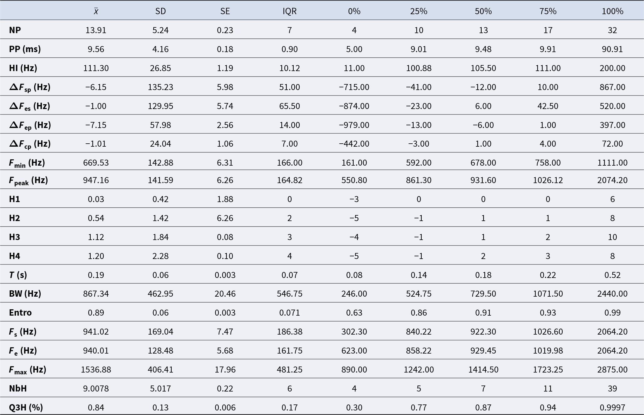
In the Ustica recordings, /kwa/ sounds occurred at rates from 0.3 to 47.7 per minute (mean ± SD: 5.5 ± 11.5). The Ustica /kwa/ sounds were pulse trains lasting 0.2 ± 0.06 s, with a peak frequency of 947.2 ± 141.6 Hz (Figure 2). Each sound comprised 13.9 ± 5.2 pulses, with an average PP of 9.3 ± 4.1 ms. Detailed acoustic characteristics are summarized in Table 1.
(a) Three spectrograms of /kwa/ sounds recorded at Ustica Island in 1999 (FFT = 256, overlap = 50%, Hann window). (b) Oscillogram of a /kwa/ sound recorded at Ustica Island in 1999.

Figure 2 Long description
Spectrogram plot in image A. The horizontal axis label is time (s), ranging from 0 to 1.6. The vertical axis label is frequency (kHz), ranging from 0 to 2.8 with tick labels at 0, 0.4, 0.8, 1.2, 1.6, 2.0, 2.4 and 2.8. The spectrogram contains three main vertical sub-panels separated across the time axis, with the /kwa/ sound visible as repeated curved stripe patterns within each sub-panel. Waveform plot in image B. The horizontal axis label is time (s), ranging from 0 to 0.30 with tick labels at 0, 0.05, 0.10, 0.15, 0.20, 0.25 and 0.30. The vertical axis label is Relative intensity (percent), ranging from negative 90 to 90 with tick labels at negative 90, negative 60, negative 30, 0, 30, 60 and 90. A single oscillating trace is centered around 0 and illustrates a /kwa/ sound recorded at Ustica Island in 1999,
Summary statistics of the acoustic features of /kwa/ sounds with at least four pseudo-harmonics

Table 1 Long description
Summary statistics for 512 /kwa/ sounds with at least four pseudo-harmonics are reported for multiple acoustic measures, including number of pulses, pulse period, frequency measurements, bandwidth, entropy, and harmonic-related measurements. Mean peak is around 947.16 Hz with a median of 931.60 Hz. Mean Fmin is around 669.53 Hz (median 678.00 Hz), while mean Fmax is around 1536.88 Hz (median 1414.50 Hz; maximum 2875.00 Hz). Bandwidth is broad and dispersed (mean 867.34 Hz; middle half from 524.75 to 1071.50 Hz; maximum 2440.00 Hz). Mean duration is around 0.19 s (middle half from 0.14 to 0.22 s; maximum 0.52 s).
N = 512. IQR, interquartile range; SD, standard deviation; SE, standard error.
Temporal description
During the 4 days and 3 nights of recordings, /kwa/ sounds were present both day and night, occurring during almost all of the analysed hours. However, their abundance showed marked diel variations (Figure 3). /Kwa/ sounds were most abundant at night, with a pronounced peak between 7 PM and 9 PM GMT (9–11 PM local time), corresponding to the beginning of the first peak in ambient noise observed each night (Figure 3). These 2 h represent only 8.33% of a 24-h cycle but accounted for 78.31% of all recorded sounds. A graphical comparison of /kwa/ sound abundance and ambient noise levels shows that the /kwa/ peak between 7 and 9 PM GMT coincides with the onset of the first nightly increase in overall sound levels (Figure 3).
Number of /kwa/ sounds per minute (right axis, blue) over time (GMT), compared to the normalized total power (left axis, in dB, black). Adapted from Hermand (Reference Hermand2003), CRC Press. Grey dots represent raw data points.

Figure 3 Long description
Normalized total power (decibel) and number of sounds per minute plotted against geotime (hour). The horizontal axis is labeled geotime (hour), with tick labels 18, 00, 06, 12, 18, 00, 06, 12, 18, 00, 06, 12. The left vertical axis is labeled Normalized total power (decibel), ranging from 0 to 1.0 with tick labels 0, 0.2, 0.4, 0.6, 0.8, 1.0. The right vertical axis is labeled Number of /kwa/ sounds per minute, ranging from 0 to 100 with tick labels 0, 20, 40, 60, 80, 100. A black line with many small grey point markers follows the left axis. It represents the normalized total power. The black line forms three repeating daily cycles across the time range. In each cycle, the black line rises from near 0 to near 1.0, then falls back toward 0, with additional smaller fluctuations between the main rises. A blue series uses the right axis and consists of vertical blue stems with circular markers. It represents the number of sounds. Blue markers appear at multiple times, generally between 19 and 21 h and similarly repeated across the subsequent day segments. Text above the plot shows three date labels: Sept. 23rd, Sept. 24th and Sept. 25th.
Temporal trends were similar across nights in terms of abundance and contribution to the soundscape, consistent with findings from a previous study (Hermand, Reference Hermand2003). No clear differences were observed between nights regarding most acoustic features. Of the 24 features calculated, only 4 showed significant differences: relative RLrms, relative SCL, entropy, and maximum frequency (Table 2, Kruskal–Wallis: χ2 = 22.22, 20.70, 6.67 & 6.22; p < 0.001, < 0.001, 0.04, and 0.04, respectively); and all four variables are known to be highly correlated (Di Iorio et al., Reference Di Iorio, Raick, Parmentier, Boissery, Valentini-Poirier and Gervaise2018).
Comparisons of /kwa/ acoustic features between the 3 nights (‘temporal’ column, Kruskal–Wallis tests, df = 2) and between Ustica and French /kwa/ sounds (‘spatial’ column, Wilcoxon–Mann–Whitney tests)

Table 2 Long description
Acoustic features of the /kwa/ sound are compared in two ways: changes across three recording nights and differences between Ustica and French recordings. For the across-nights tests, most features show no clear change, with p-values above 0.05 for Fpeak, NP, PP, multiple delta frequency measures, Fmin, H2, H3, H4, T, BW, Fs, Fe, NbH, Q3H and relative SNR. Significant across-night differences appear for Entro (p 0.04) and Fmax (p 0.04), and very strong differences for relative RLrms and relative SCL (both p less than 0.001). For the location comparison, several features differ strongly between Ustica and French datasets, including Fpeak, PP, Fmin, T, Fs, and Fe (all mean p-values less than 0.001), with Entro (mean p-value 0.004) and Fmax also differing (mean p-value 0.01). Other location comparisons are not different, such as NP, the delta frequency measures, BW, H2, H3, H4, NbH, and Q3H (mean p-values 0.13 to 0.53).
For the between-nights comparison, only data recorded between 7 PM and midnight GMT have been used. For the spatial comparison, five groups of 512 observations from both French and Ustica datasets were compared using bootstrap Wilcoxon–Mann–Whitney tests. p-values <0.05 are indicated in bold.
The 2-h period of high sound production begins approximately 2 h after sunset (based on sunset times for Palermo, Northern Sicily; NOAA/GML Solar Calculator). The duration of this period and its position within the day/night cycle are similar to the choruses described in southern metropolitan France (Di Iorio et al., Reference Di Iorio, Raick, Parmentier, Boissery, Valentini-Poirier and Gervaise2018), Corsica (Di Iorio et al., Reference Di Iorio, Raick, Parmentier, Boissery, Valentini-Poirier and Gervaise2018), and in Italian meadows (Ceraulo et al., Reference Ceraulo, Papale, Caruso, Filiciotto, Grammauta, Parisi, Mazzola, Farina and Buscaino2018). In winter, /kwa/ sounds are known to occur sporadically, with no choruses being recorded (Ceraulo et al., Reference Ceraulo, Papale, Caruso, Filiciotto, Grammauta, Parisi, Mazzola, Farina and Buscaino2018). This period and duration are also similar to those observed for kwa-like sounds from tropical reefs (Raick et al., Reference Raick, Di Iorio, Lecchini, Gervaise, Hédouin, Under The Pole, Pérez-Rosales, Rouzé, Bertucci and Parmentier2023, Reference Raick, Campisi, Under The Pole, Bertucci, Lecchini, Di Iorio and Parmentier2025).
Both RL and SCL, which represent the intensity levels of sound emission, differed significantly between nights. The fact that only this subset of features varies, while all others remain consistent, indicates that the /kwa/ sounds are essentially similar across nights in terms of duration, frequency, and shape, but differ in intensity. This finding aligns with observations of French /kwa/ choruses, where intensity varies from night to night (Di Iorio et al., Reference Di Iorio, Raick, Parmentier, Boissery, Valentini-Poirier and Gervaise2018). At a broader time scale, RL is known to peak in July, being higher in summer than in spring. However, more data are needed to better understand not only potential seasonal variations but also those occurring over shorter time frames.
Comparison with /kwa/ sounds from French meadows
When comparing /kwa/ sounds from Ustica and the French littoral, several differences were observed. First, all the frequency-related features (F min, F peak, F max, F s, F e) were significantly different (Table 2), with /kwa/ frequencies in Ustica being higher than those in France. All other features were equivalent, except for duration (T), entropy (Entro), and PP. The PP of /kwa/ in Ustica was shorter than in France (9.56 ± 4.16 ms compared to 13 ± 4 ms). The same was observed for T (0.19 ± 0.064 s vs. 0.27 ± 0.09 s) and the contrary for Entro (89.1 ± 6.1 vs. 86.6 ± 5.6). Notably, Ustica /kwa/ sounds exhibited the highest F peak values and the shortest durations. Entropy, duration, and frequency features (such as F peak) in Ustica /kwa/ were similar to those recorded at an equivalent period in the French meadows (Figure 4).
Normalized mean (ranging from 0 to 1) and standard deviation of selected key acoustic features from the French littoral as a function of time (adapted from Di Iorio et al. (Reference Di Iorio, Raick, Parmentier, Boissery, Valentini-Poirier and Gervaise2018): F peak in orange, PP in blue, BW in yellow, NP in green, and Entropy in grey. The red box highlights the Ustica data.

Figure 4 Long description
The multi-line graph presents normalized mean values of selected acoustic features from March to September. The x-axis represents months, while the y-axis shows normalized units ranging from negative 0.3 to 1.1. The top section compares Fpeak and PP as well as temperature (°C, right axis). The middle section displays BW and NP . The bottom section illustrates RL and Entropy . The red box highlights data from Ustica. Key trends include Fpeak′s increase, RL′s peak in July, and a decline for PP . The graph aims to demonstrate variations in acoustic features over time, highlighting fluctuation among the metrics.
The frequencies of Ustica /kwa/ sounds were higher than those recorded in the French datasets, a pattern also observed for PP. Variability in both F peak and PP has already been reported for French /kwa/ sounds (Di Iorio et al., Reference Di Iorio, Raick, Parmentier, Boissery, Valentini-Poirier and Gervaise2018), with F peak tending to be higher in summer than in spring, while the opposite trend was observed for PP. This seasonal variation was demonstrated in specific meadows in the South of France (Parc Marin de la Côte Bleue) and Corsica (Calvi), as well as through comparisons between different meadows. The peak frequency of the Ustica /kwa/ sounds was more than 100 Hz higher than that reported by Ceraulo et al. (Reference Ceraulo, Papale, Caruso, Filiciotto, Grammauta, Parisi, Mazzola, Farina and Buscaino2018) for the corresponding ‘MF-fish sounds’ (mean ± SE: 840 ± 75.37) (Ceraulo et al., Reference Ceraulo, Papale, Caruso, Filiciotto, Grammauta, Parisi, Mazzola, Farina and Buscaino2018); however, their data were collected over several months, which may have averaged out F peak values. The difference in F peak was smaller when compared with croak sounds recorded in Spain (González Correa et al., Reference González Correa, Bayle Sempere, Juanes, Rountree, Ruíz and Ramis2019) (mean ± SE: 900 ± 145.7 Hz), which are now considered synonymous with the /kwa/ sound type (Bolgan et al., Reference Bolgan, Soulard, Di Iorio, Gervaise, Lejeune, Gobert, Parmentier, Di Iorio, Gervaise, Lejeune, Gobert and Parmentier2019). It has also been shown that /kwa/ sounds recorded in Crete differ from those recorded in the western basin (Corsica and Mallorca) in terms of frequency characteristics (e.g., peak frequency) and temporal features (e.g., PP) (Bolgan et al., Reference Bolgan, Di Iorio, Dailianis, Catalan, Lejeune, Picciulin and Parmentier2022). While this sound dominated the 700–900 Hz range at western sites, it was most frequently observed between 900 and 1100 Hz in Crete (Bolgan et al., Reference Bolgan, Di Iorio, Dailianis, Catalan, Lejeune, Picciulin and Parmentier2022).
The previously mentioned features are influenced by the temperature [4]; as temperature increases, both the velocity and activation rate of fish muscles also increase. In Ustica, water temperatures in September are typically higher than those recorded at all French sites, including during the warmest months. Consequently, it is expected that temperature-dependent features would increase (F peak) or decrease (PP) in the Ustica recording. However, the difference in PP between Ustica and the French data is so substantial that it may also indicate an intrinsic difference. It is possible that, due to spatial separation, the populations of fish producing /kwa/ sounds are different, either two closely related species or distinct populations of the same species (Bolgan et al., Reference Bolgan, Di Iorio, Dailianis, Catalan, Lejeune, Picciulin and Parmentier2022). One of these species is Scorpaena maderensis, a subtropical species from the eastern Atlantic and parts of the Mediterranean Sea, including areas such as Greece, Spain, and Sicily (Hureau and Litvinenko, Reference Hureau, Litvinenko, White-head, Bauchot, Hureau, Nielsen and Tortonese1986; La Mesa et al., Reference La Mesa, Micalizzi, Giaccone and Vacchi2004). In 2001, S. maderensis was the most abundant cryptobenthic fish species off northern Sicily, far exceeding the abundance of species such as S. porcus (La Mesa et al., Reference La Mesa, Micalizzi, Giaccone and Vacchi2004). Off Corsica, where a significant portion of the comparative data used in this study originates, this species was first documented in 2003. By 2018, it had become the most prevalent Scorpaenidae species observed along the region’s rocky coast (Astruch et al., Reference Astruch, Belloni, Rouanet, Schohn, Harmelin‐Vivien, Harmelin and Boudouresque2022).
The higher peak frequencies and smaller PPs found in Ustica may therefore linked either to higher temperatures or to species/population differences compared to other Mediterranean sites. To differentiate between the two, more research is needed. First, to better understand the source of /kwa/ sounds at a fine species and population level within Scorpaenidae. Second, to better understand the seasonality of /kwa/ sounds in relation to temperature. These two lines of investigation are not independent and may potentially reveal a dual effect of global change on the biophony of P. oceanica meadows. Rising temperatures may impact sonic mechanisms at the physiological level, leading to increases in peak frequencies. A previous study found that when the abundance of the /kwa/ was higher, the range of spectral and temporal acoustic resources it exploited was also broader (Bolgan et al., Reference Bolgan, Di Iorio, Dailianis, Catalan, Lejeune, Picciulin and Parmentier2022). However, it remains unclear whether the sonic system possesses sufficient plasticity to accommodate higher frequencies. On the other hand, increasing temperatures are known to alter the relative abundance of Scorpaena species in shallow fish assemblages, which may further affect biophony, especially if all species within the genus produce this sound type. The two research directions highlighted above – the relationship between species differences in Scorpaena and the variability of /kwa/ sounds, and the influence of water temperature on the acoustic characteristics of /kwa/ sounds – are crucial for understanding potential modifications of soundscapes in the context of global change.
Acknowledgements
We thank Laura Velasi for comments on a previous version of the manuscript.
Author contributions
X.R. and J.-P.H. conceived the study. X.R. performed the acoustic and statistical analyses under the supervision of L.D.I. X.R. wrote the manuscript. Both L.D.I. and J.-P.H. contributed to the final version of the manuscript. All authors provided critical feedback and helped shape the research, analysis, and manuscript. X.R. supervised the project.
Declaration of interest
The authors declare that they have no conflicts of interest.
Data availability statement
The data supporting the findings of this study are available in Hermand (Reference Hermand2003) and Di Iorio et al. (Reference Di Iorio, Raick, Parmentier, Boissery, Valentini-Poirier and Gervaise2018). Additional data are available from the corresponding author upon reasonable request.
Ethics and approach
No ethical approval was required for this study, as passive acoustic monitoring is a non-invasive method and did not involve direct interaction with animals or humans.
Funding statement
We did not receive any funding for this specific work. During the final stages of the research, X.R. was funded by a Belgian American Educational Foundation fellowship and a Wallonia-Brussels International fellowship.




 Open access

