


1. Introduction
Incomplete and noisy information about a system is frequent in the analysis of fluid systems. Experiments typically involve partial access to flow information: hot-wire anemometry provides high sensitivity and time resolution, but for a limited number of spatial locations; particle image velocimetry (PIV) can provide considerably improved spatial resolution, but generally suffers from lower signal-to-noise ratio and sampling frequency. Stationary properties of the flow, such as the mean flow, can be obtained by moving sensors over a region of interest, and two-point statistics can be obtained by moving pairs of sensors. The process is tedious, time consuming and does not permit a time-resolved estimation of the flow state. It is therefore of interest to develop methods capable of estimating flow information from limited and noisy measurements.
Estimation has a long history. Landmark developments were obtained independently by Wiener (Reference Wiener1942) and Kolmogorov (Reference Kolmogorov1941), equivalent results being later obtained by Kalman (Reference Kalman1960) for problems where a system's time evolution is known; this restriction permits a simpler framework and is likely the reason for the more widespread use of the Kalman filter. These methods constitute optimal linear estimators for generic error norms. Assuming a known initial condition and an external forcing characterised by zero-mean Gaussian statistics, the two-point correlation of the state can be obtained by solution of a Riccati equation. Wiener and Kalman approaches can be shown to be equivalent (Gómez Reference Gómez2007). Specifically, the causal Wiener filter is equivalent to the Kalman filter and the non-causal Wiener filter is equivalent to the Kalman smoother.
Within Kalman's framework, estimation is categorised into three classes, depending on the information available for estimation of the state at time  $t_0$. If information is available for all
 $t \leq t_0$, estimation is referred to as a filter; if readings are available for
 $t<t_1$, with
 $t_1>t_0$, estimation is referred to as data smoothing; and if
 $t_1<t_0$, estimation is referred to as a prediction. The method we develop is a smoother with an infinite time horizon: information for
 $-\infty < t < \infty$ is assumed to be available. Note that the nomenclature used in Wiener's framework is different: a Wiener filter performs non-causal estimation, while a causal Wiener filter provides causal estimation.
The greater popularity of causal estimation is explained by its utility for flow control. Linear quadratic Gaussian (LQG) control can be implemented using Kalman-filter estimation, coupled with a linear quadratic regulator (LQR), which calculates optimal control based on state estimation (Hespanha Reference Hespanha2009). Linear quadratic Gaussian control of fluid systems has become widespread in recent years, particularly for delaying boundary layer transition and reducing drag (see, for instance, Fabbiane etal. Reference Fabbiane, Simon, Fischer, Grundmann, Bagheri and Henningson2015b; Fabbiane, Bagheri & Henningson Reference Fabbiane, Simon, Fischer, Grundmann, Bagheri and Henningson2015a). However, implementation is complicated by the large dimensionality of fluid systems. Traditional LQG methods require the solution of two Riccati equations, which is frequently too costly for direct application on flow systems of practical interest. An alternative approach involves the use of a reduced-order model (ROM), typically obtained by Galerkin projection of the system on a reduced basis. Bases can be constructed using eigenmodes of the observability and controllability Gramians, or balanced modes (Bagheri etal. Reference Bagheri, Henningson, Hœpffner and Schmid2009). Other possibilities include flow eigenmodes (Åkervik etal. Reference Åkervik, Hœpffner, Ehrenstein and Henningson2007), proper orthogonal decomposition (POD) modes (Kirby, Boris & Sirovich Reference Kirby, Boris and Sirovich1990), spectral proper orthogonal decomposition (SPOD) modes and a spectral version of balanced truncation modes (Dergham etal. Reference Dergham, Sipp, Robinet and Barbagallo2011). Balanced modes provide a quasi-optimal choice, having an a priori error bound (Sipp & Schmid Reference Sipp and Schmid2016). Eigensystem realisation algorithms (ERA) (Juang & Pappa Reference Juang and Pappa1985) have been shown to be equivalent to ROM based on balanced truncation (Ma, Ahuja & Rowley Reference Ma, Ahuja and Rowley2011), and have the advantage of being less costly and of avoiding the need to integrate adjoint systems. Matrix-free methods have been developed that permit optimal (Semeraro etal. Reference Semeraro, Pralits, Rowley and Henningson2013) and robust (Bewley, Temam & Ziane Reference Bewley, Temam and Ziane2000) flow control via iteration of the system's direct and adjoint equations. The ensemble Kalman filter approximates error covariances using a reduced ensemble, and this can be used to provide an approximation of Kalman-filter estimates (da Silva & Colonius Reference da Silva and Colonius2018).
In a number of recent studies of turbulent flows, flow models are obtained by linearising the Navier–Stokes equations about the time-averaged mean, and subjecting the resulting linear operator to an external forcing that would model the effects of nonlinearity. In the frequency domain, this problem can be formulated such that the resolvent of the linear operator appears as a transfer function between nonlinear forcing and linear response. Large gain separation between optimal and suboptimal resolvent force-response mode pairs implies a system whose response will be relatively insensitive to specifics of the forces; such a system tends to exhibit low-rank behaviour. This approach was first used by McKeon & Sharma (Reference McKeon and Sharma2010) in the study of wall-bounded turbulence, and later extended to non-parallel flows (Beneddine etal. Reference Beneddine, Sipp, Arnault, Dandois and Lesshafft2016). Similar ideas have been used to model turbulent jets (Towne, Schmidt & Colonius Reference Towne, Schmidt and Colonius2018; Cavalieri, Jordan & Lesshafft Reference Cavalieri, Jordan and Lesshafft2019; Lesshafft etal. Reference Lesshafft, Semeraro, Jaunet, Cavalieri and Jordan2019), to perform flow estimation with low computational cost (Beneddine etal. Reference Beneddine, Yegavian, Sipp and Leclaire2017; Sasaki etal. Reference Sasaki, Cavalieri, Jordan, Schmidt, Colonius and Brès2017a), to elaborate simplified control strategies (Sasaki etal. Reference Sasaki, Tissot, Cavalieri, Silvestre, Jordan and Biau2016) and for the modelling and estimation of a turbulent flow over an airfoil (Abreu, Cavalieri & Wolf Reference Abreu, Cavalieri and Wolf2017; Beneddine etal. Reference Beneddine, Yegavian, Sipp and Leclaire2017; Yeh & Taira Reference Yeh and Taira2019). In most of these studies it is assumed that the system has rank-1 behaviour at each frequency; thus, the cross-spectral density matrix can be approximated by considering a single resolvent mode, which corresponds to the dominant response mode of the system. Although not optimal, the lower costs of these approaches makes them attractive.
All of the methods described above have advantages and disadvantages: control using reduced-order models is not guaranteed to be optimal for the full system and the computation of large numbers of POD or eigenmodes can be costly; the frequency snapshot method is limited to low-rank forces, as harmonic responses for many frequencies need to be computed for each force component; matrix-free methods require routines to integrate the adjoint equations, they require many iterations to ensure convergence, and they are limited to low-rank external forces; and ERA methods are useful when external forces are low rank, but become prohibitively expensive otherwise. Low-rank approximations based on optimal response modes are not optimal, and can, depending on sensor placement, become unstable if a higher-rank model is used, as will be shown later. In all of these methods, force colouring can only be accounted for via a system expansion, in which a filter colours white-noise inputs. For an overview of estimation with coloured forces, we refer the reader to Kailath & Geesey (Reference Kailath and Geesey1971) and Kailath (Reference Kailath1974). One exception is the work of Hervé etal. (Reference Hervé, Sipp, Schmid and Samuelides2012), where a data-driven approach is elaborated based on an autoregressive moving average (ARMAX) system identification. Force colour effects are captured indirectly via data processing. Although effective, the approach does not provide insight regarding the underlying physical mechanisms.
Smoothers have received considerably less attention, particularly in the fluid mechanics community. In the Wiener framework, Bode & Shannon (Reference Bode and Shannon1950) presented a simplified derivation of a smoothing theory. Fraser & Potter (Reference Fraser and Potter1969) showed that Kalman smoothing is equivalent to the combination of two Kalman filters, one moving forward and another backward in time. Bell (Reference Bell1994) proposed an iterative Gauss–Newton method for the performance of Kalman smoothing. Pnevmatikakis etal. (Reference Pnevmatikakis, Rad, Huggins and Paninski2014) developed efficient filtering and smoothing techniques that can be obtained when the covariance between states and measurements is low rank, or permits a low-rank approximation: this can be a consequence of low-rank forces, large measurement noise or due to the way the system filters the forces.
While variations on the Kalman filter have been used in many studies to estimate flow state, to the best of the authors’ knowledge, the only application of the Wiener filter (causal and non-causal) is that of Martinelli (Reference Martinelli2009), where Wiener methods were applied to a turbulent channel flow. The study was restricted to the use of only one sensor and actuator, probably due to the complexity of solving higher-order Wiener–Hopf problems, and was, furthermore, restricted to a low-dimensional problem, as for flows with more than one inhomogeneous spatial dimension, the construction and manipulation of the system matrices becomes prohibitive. A similar method has recently been used to improve PIV data (Gillissen, Bouffanais & Yue Reference Gillissen, Bouffanais and Yue2019), but no explicit mention of Wiener's work was made.
In this work we explore estimation of linear systems, with an infinite time horizon: there are no transient effects, and readings for times before and after the estimated instant are available, i.e. in the post-processing of experimental data. Building on works by Beneddine etal. (Reference Beneddine, Sipp, Arnault, Dandois and Lesshafft2016, Reference Beneddine, Yegavian, Sipp and Leclaire2017) and Towne, Lozano-Durán & Yang (Reference Towne, Lozano-Durán and Yang2020) we derive an expression for force estimation considering underlying force statistics and sensor noise by looking for a stationary point of the error correlation matrix for forces and responses, and we show that optimal state estimation is obtained from the integration of estimated forces. The estimation kernels are obtained analytically in the frequency domain, with a corresponding time-domain representation obtained a posteriori by an inverse Fourier transform. When the forcing statistics are known, the method is shown to be equivalent to a multiple-input, multiple-output Wiener filter. On the other hand, when the forcing statistics are unknown and approximated as white, the method is equivalent to constructing an approximate Wiener filter using estimated statistics obtained from the resolvent-based statistical estimation method developed by Towne etal. (Reference Towne, Lozano-Durán and Yang2020). Contrary to previous work (Bagheri etal. Reference Bagheri, Henningson, Hœpffner and Schmid2009; Dergham etal. Reference Dergham, Sipp, Robinet and Barbagallo2011; Sipp & Schmid Reference Sipp and Schmid2016), no model reduction is performed: estimation is performed using the full system, without the need of iterative methods and subsequent integration of the estimation equations, as in Semeraro etal. (Reference Semeraro, Pralits, Rowley and Henningson2013).
The paper is organised as follows. In § 2 we present the derivation of optimal state and force estimations. In § 3 we provide a comparison between causal (Kalman-filter) and non-causal (resolvent-based) estimations of a stochastically forced, linearised Ginzburg–Landau model. The kernels of the two approaches are compared in § 3.3. In § 3.4 we compare the proposed method to truncation methods reported in the literature. The method is then applied to two fluid mechanics problems in § 4: a linearised, spatially evolving boundary layer is considered in § 4.1; and a turbulent channel flow in § 4.2. Conclusions are provided in § 5.
2. Resolvent-based estimation
Here we derive optimal methods for the recovery of system states and driving forces. As in previous studies (Kalman Reference Kalman1960; Bagheri etal. Reference Bagheri, Henningson, Hœpffner and Schmid2009; Murray Reference Murray2009), we work with the linear time-invariant model
 \begin{gather} \dfrac{\textrm{d}\boldsymbol{u}}{\textrm{d}t}(t) = \boldsymbol{\mathsf{A}} \boldsymbol{u}(t) + \boldsymbol{\mathsf{B}}\, \boldsymbol{f}(t), \end{gather}
 \begin{gather} \boldsymbol{y}(t) = \boldsymbol{\mathsf{C}} \boldsymbol{u}(t) + \boldsymbol{n}(t), \end{gather}
where  $\boldsymbol{\mathsf{A}},\boldsymbol{\mathsf{B}}$ and
 $\boldsymbol{\mathsf{C}}$ are the system evolution (
 $n_u\times n_u$), actuation (
 $n_u\times n_b$) and observation (
 $n_c\times n_u$) matrices,
 $\boldsymbol {u}$ and
 $\boldsymbol {y}$ are, respectively, the system state (
 $n_u$) and observation (
 $n_y$) vectors. Vectors
 $\boldsymbol {f}$ and
 $\boldsymbol {n}$ represent, respectively, the system's driving forces (
 $n_b$) and measurement noise (
 $n_y$), which are considered as zero-mean random processes with
 \begin{equation}\langle\, \boldsymbol{f}(t) \boldsymbol{f}(t')^{\dagger}\rangle = \boldsymbol{\mathsf{F}}(t-t'), \quad \langle \boldsymbol{n}(t) \boldsymbol{n}(t')^{\dagger} \rangle = \boldsymbol{\mathsf{N}}(t-t'),\quad \langle \boldsymbol{n}(t) \boldsymbol{f}^{\dagger}(t') \rangle =0, \end{equation}
where ‘ $\dagger$’ indicates the adjoint operator, where an unweighted inner product is assumed. Here
 $\boldsymbol{\mathsf{F}}(t-t')$ and
 $\boldsymbol{\mathsf{N}}(t-t')$ are Hermitian positive-definite matrices. In the control literature (2.1) is typically written using
 $\boldsymbol {x}$ and
 $\boldsymbol {d}$ to represent the system state and external disturbances,
 $\boldsymbol {u}$ denoting actuation. In this study we use the nomenclature presented above, which has become standard in fluid mechanics. Figure 1 presents a flowchart illustrating the system and the estimation that will be presented in the next subsections. We also assume that all variables and matrices are complex; real-valued matrices and vectors, as is the case in the Navier–Stokes system, is a special case.
Flowchart illustrating the system considered and the estimation proposed.

The forms used in (2.3) imply a more general framework than that of the Kalman filter, where forces are assumed to be uncorrelated in time and space, i.e.  $\boldsymbol{\mathsf{F}}(t-t')=\boldsymbol{\mathsf{I}}\delta (t-t')$, similar expressions are used to describe other cross-correlations. Coloured-force methods exist in the Kalman framework. Typically, an extended system can be obtained in which a filter is used to colour a white-noise force prior to application; the approach we propose handles force colour naturally. Forces and readings are assumed to be uncorrelated throughout the paper; but expressions obtained when this correlation is non-zero are provided in appendix A. Finally, we restrict our attention to stable systems: all eigenvalues of
 $\boldsymbol{\mathsf{A}}$ have a negative real part.
In what follows, we derive independent methods for optimal force and response estimations based on the time history of low-rank observations,  $\boldsymbol {y}(t)$.
2.1. Force estimation
Defining the instantaneous error,  $\boldsymbol{e}_f(t)$, between the force,
 $\boldsymbol {f}(t)$, and its estimation,
 $\tilde {\boldsymbol {f}}(t)$, as
 \begin{equation} \boldsymbol{e}_f(t) = \boldsymbol{f}(t)-\tilde{\boldsymbol{f}}(t), \end{equation}
we seek an optimal estimation such that a stationary point of the time-averaged error correlation matrix
 \begin{equation} \langle\boldsymbol{e}_f \boldsymbol{e}_f^{\dagger}\rangle=\int_{-\infty}^{\infty} \langle \boldsymbol{e}_f(t) \boldsymbol{e}_f^{\dagger}(t)\rangle\, \textrm{d}t = \dfrac{1}{2\pi}\int_{-\infty}^{\infty} \langle\hat{\boldsymbol{e}}_f(\omega)\hat{\boldsymbol{e}}_f^{\dagger} (\omega)\rangle\,\textrm{d}\omega \end{equation}
is found. Note that this is a generalization of root-mean-square errors, which is given by the trace of  $\langle \boldsymbol {e}_f \boldsymbol {e}_f^{\dagger }\rangle$. The integration limits reflect the estimation objective: to estimate
 $\boldsymbol {f}(t)$ for all times. Here
 $\langle \cdot \rangle$ represents an ensemble average,
 $\hat{\boldsymbol{e}}_{f}(\omega)$ is the Fourier transform of
 $\boldsymbol{e}_{f}(t)$, defined by
 \begin{equation} \hat{\boldsymbol{e}}_f (\omega) = \int_{-\infty}^{\infty} \boldsymbol{e}_f(t) \mathrm{e}^{ {\mathrm{i}} \omega t}\,\textrm{d}t, \end{equation}
and the equivalence of the time and frequency domains in (2.5) is given by Parseval's theorem (Arfken, Weber & Harris Reference Arfken, Weber and Harris2013, p. 595). No assumption is made regarding the underlying probability functions of forces, responses and errors. As discussed by Kalman (Reference Kalman1960), this provides the optimal estimation if forces are Gaussian distributed. For other force distributions, optimal estimation is nonlinear, the method above providing the optimal linear estimation. Note that this is analogous to a least-squares method for fitting curves: if errors have a Gaussian distribution, the method is equivalent to a maximum-likelihood method; however, the method is still effective for other distributions.
Formal solutions of (2.1) in time and frequency domains are obtained as
 \begin{equation}\boldsymbol{u}(t) = \int_{-\infty}^{t} e^{\boldsymbol{\mathsf{A}} (t-\tau)}\boldsymbol{\mathsf{B}}\, \boldsymbol{f}(\tau)\,\textrm{d}\tau,\quad \hat{\boldsymbol{u}} (\omega) = \boldsymbol{\mathsf{R}} (\omega) \boldsymbol{\mathsf{B}}\,\hat{f}(\omega), \end{equation}
where  $\boldsymbol{\mathsf{R}} = (-\boldsymbol{\mathsf{A}} -\mathrm {i}\omega \boldsymbol{\mathsf{I}})^{-1}$. We assume a time evolution from
 $-\infty$ to
 $\infty$, where an initial condition,
 $\boldsymbol {u}_0$, at time,
 $t_0$, can be represented via a forcing,
 $\boldsymbol{\mathsf{B}} \,\boldsymbol {f}(t)=\boldsymbol {u}_0\delta (t-t_0)$.
Considering the state  $\tilde {\boldsymbol {u}}$ obtained by integration of an estimated force
 $\tilde {\boldsymbol {f}}$,
 \begin{equation} \tilde{\boldsymbol{u}}(t) = \int_{-\infty}^{t} e^{\boldsymbol{\mathsf{A}} (t-\tau)}\boldsymbol{\mathsf{B}} \,\tilde{\boldsymbol{f}}(\tau)\, \textrm{d}\tau,\quad \hat{\tilde{\boldsymbol{u}}} (\omega) = \boldsymbol{\mathsf{R}} (\omega) \boldsymbol{\mathsf{B}}\, \hat{\tilde{\boldsymbol{f}}}(\omega), \end{equation}
we seek to obtain  $\tilde {\boldsymbol {f}}$ as a linear function of the readings
 \begin{equation}\tilde{\boldsymbol{f}}(t) = \int_{-\infty}^{\infty} \boldsymbol{\mathsf{T}}_{\boldsymbol{f}} (t-\tau) \boldsymbol{y}(\tau)\, \textrm{d}\tau,\quad \hat{\tilde{\boldsymbol{f}}}(\omega) = \skew4\hat{\boldsymbol{\mathsf{T}}}_{\boldsymbol{f}} (\omega) \hat{\boldsymbol{y}}(\omega), \end{equation}
such that the estimation problem involves finding an estimation function,  $\skew3\hat {\boldsymbol{\mathsf{T}}}_{\boldsymbol {f}}(\omega )$, that would minimise the norm of
 $\langle \hat {\boldsymbol {e}}_f \hat {\boldsymbol {e}}_f^{\dagger } \rangle$. Note that the estimation function in (2.9) is generally non-causal.
The error correlation matrix is rewritten, with frequency dependencies omitted for clarity, as
 \begin{align} \left\langle\hat{\boldsymbol{e}}_f \hat{\boldsymbol{e}}_f^{\dagger}\right\rangle & = \left\langle \left(\skew2\hat{\boldsymbol{f}} - \skew4\hat{\boldsymbol{\mathsf{T}}}_{\boldsymbol{f}} \left(\boldsymbol{\mathsf{R}}_{\boldsymbol{y}}\skew2\hat{\boldsymbol{f}}+\hat{\boldsymbol{n}} \right)\right) \left(\skew2\hat{\boldsymbol{f}} - \skew4\hat{\boldsymbol{\mathsf{T}}}_{\boldsymbol{f}} \left(\boldsymbol{\mathsf{R}}_{\boldsymbol{y}}\, \skew2\hat{\boldsymbol{f}}+\hat{\boldsymbol{n}} \right) \right)^{\dagger} \right\rangle, \nonumber\\ &= \left(\boldsymbol{\mathsf{I}} -\skew4\hat{\boldsymbol{\mathsf{T}}}_{\boldsymbol{f}} \boldsymbol{\mathsf{R}}_{\boldsymbol{y}} \right) \skew4\hat{\boldsymbol{\mathsf{F}}} \left(\boldsymbol{\mathsf{I}} -\skew4\hat{\boldsymbol{\mathsf{T}}}_{\boldsymbol{f}} \boldsymbol{\mathsf{R}}_{\boldsymbol{y}} \right)^{\dagger} + \skew4\hat{\boldsymbol{\mathsf{T}}}_{\boldsymbol{f}} \skew3\hat{\boldsymbol{\mathsf{N}}} \skew4\hat{\boldsymbol{\mathsf{T}}}_{\boldsymbol{f}}^{\,\dagger}. \end{align}
The operator  $\boldsymbol{\mathsf{R}}_{\boldsymbol {y}} = \boldsymbol{\mathsf{C}}\boldsymbol{\mathsf{R}} \boldsymbol{\mathsf{B}}$ relates forces to sensor readings, and the matrices
 $\skew4\hat {\boldsymbol{\mathsf{F}}}(\omega )$ and
 $\skew4\hat {\boldsymbol{\mathsf{N}}}(\omega )$ are Fourier transforms of
 $\boldsymbol{\mathsf{F}}(t)$ and
 $\boldsymbol{\mathsf{N}}(t)$, defined in (2.3). Typically, the forcing rank is much larger than the number of sensors,
 $n_y \ll n_b$, and, thus, it is natural that the forcing cannot be fully estimated. The estimation is limited to the subspace of observable forces (Towne etal. Reference Towne, Lozano-Durán and Yang2020). By definition, any force that generates a non-zero sensor reading has a non-zero projection in this subspace.
A connection can be made with the observability Gramian (Bagheri etal. Reference Bagheri, Henningson, Hœpffner and Schmid2009), which is obtained through a time integral
 \begin{equation} \mathcal{G} = \int_{0}^{\infty} \mathrm{e}^{\boldsymbol{\mathsf{A}}^{\dagger}\tau}\boldsymbol{\mathsf{C}}^{\,\dagger} \boldsymbol{\mathsf{C}} \mathrm{e}^{\boldsymbol{\mathsf{A}}\tau}\,\textrm{d}\tau. \end{equation}
Alternatively, the observability Gramian can be written using Parseval's theorem (Zhou, Salomon & Wu Reference Zhou, Salomon and Wu1999; Dergham etal. Reference Dergham, Sipp, Robinet and Barbagallo2011)
 \begin{equation} \mathcal{G} = \frac{1}{2\pi} \int_{-\infty}^{\infty} \boldsymbol{\mathsf{R}}^{\,\dagger}\boldsymbol{\mathsf{C}}^{\,\dagger} \boldsymbol{\mathsf{C}} \boldsymbol{\mathsf{R}}\,\textrm{d}\omega. \end{equation}
At a given frequency, the observable space is spanned by the eigenvectors of  $\boldsymbol{\mathsf{R}}^{\,\dagger }\boldsymbol{\mathsf{C}}^{\,\dagger } \boldsymbol{\mathsf{C}} \boldsymbol{\mathsf{R}}$ associated with non-zero eigenvalues. When viewed in the time domain through the observability Gramian, each force component is weighted by its overall observability at all frequencies. A low-rank truncation of this Gramian can be used to obtain a reduced basis for the construction of time-domain ROMs, implicitly favouring some frequencies over others. A similar reasoning applies to the construction of balanced modes (Bagheri etal. Reference Bagheri, Henningson, Hœpffner and Schmid2009). In the approach presented here, we use the full observable space at each frequency, without the aforementioned truncation.
As  $\langle \hat{\boldsymbol{e}}_f \hat{\boldsymbol {e}}_f^{\dagger}\rangle$ is a matrix, it is typically necessary to specify a minimisation criterion: minimisation of the trace, for instance, as is done in the design of Kalman filters, or of the determinant. We will show, however, that a stationary point can be obtained simultaneously for all matrix terms, illustrating a certain robustness of the method. We impose
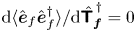 ${\textrm {d} {\langle \hat{\boldsymbol {e}}_f \hat {\boldsymbol {e}}_f^{\dagger }\rangle }}/{\textrm {d} {\skew4\hat {\boldsymbol{\mathsf{T}}}}_{\boldsymbol {f}}^{\,\dagger }}= 0$ and
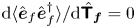 ${\textrm {d} {\langle \hat {\boldsymbol {e}}_f \hat {\boldsymbol {e}}_f^{\dagger }\rangle }}/{\textrm {d} {\skew4\hat {\boldsymbol{\mathsf{T}}}_{\boldsymbol {f}}}}= 0$, where
 ${\skew4\hat {\boldsymbol{\mathsf{T}}}}_{\boldsymbol {f}}^{\,\dagger }$ and
 ${\skew4\hat {\boldsymbol{\mathsf{T}}}_{\boldsymbol {f}}}$ are treated as independent variables (Ahlfors Reference Ahlfors1979, p. 79). It can be shown that both expressions lead to the same equation, we thus focus only on the first. As both
 $\langle \hat {\boldsymbol {e}}_f \hat {\boldsymbol {e}}_f^{\dagger }\rangle$ and
 ${\skew4\hat {\boldsymbol{\mathsf{T}}}}_{\boldsymbol {f}}^{\,\dagger }$ are matrices, the derivative is a fourth-order tensor, it is thus simpler to take the derivative using Einstein's summation convention. Equation (2.10) has the form
 \begin{equation} \left\langle\hat{\boldsymbol{e}}_f \hat{\boldsymbol{e}}_f^{\dagger}\right\rangle_{il} = \Gamma_{ij} {T_f}^{\dagger}_{jk} + \Lambda_{ik}, \end{equation}
with
 \begin{gather} \boldsymbol{\Gamma} = \skew4\hat{\boldsymbol{\mathsf{T}}}_{\boldsymbol{f}} \left( \boldsymbol{\mathsf{R}}_{\boldsymbol{y}} \skew4\hat{\boldsymbol{\mathsf{F}}} \boldsymbol{\mathsf{R}}_{\boldsymbol{y}} ^{\,\dagger} + \skew3\hat{\boldsymbol{\mathsf{N}}} \right) - \skew4\hat{\boldsymbol{\mathsf{F}}} \boldsymbol{\mathsf{R}}_{\boldsymbol{y}} ^{\,\dagger}, \end{gather}
 \begin{gather} \boldsymbol{\Lambda} = \left(\boldsymbol{\mathsf{I}}-\skew4\hat{\boldsymbol{\mathsf{T}}}_{\boldsymbol{f}} \boldsymbol{\mathsf{R}}_{\boldsymbol{y}}\right) \skew4\hat{\boldsymbol{\mathsf{F}}}. \end{gather}
The derivative is given by
 \begin{equation} \dfrac{\textrm{d} \langle\hat{\boldsymbol{e}}_f \hat{\boldsymbol{e}}_f^{\dagger}\rangle_{il}}{{\textrm{d} {\hat{T}_f}^{\dagger}}_{mn}} = \Gamma_{ij} \delta_{jm}\delta_{kn} = \Gamma_{im} \delta_{kn}, \end{equation}
where  $\delta _{ij}$ is the Kronecker delta. The expression is a tensor product between two matrices, and it is zero only if one of these is zero. As only
 $\boldsymbol{\Gamma}$ is a function of
 ${\boldsymbol{\mathsf{T}}}_{\boldsymbol {f}}$, the stationary point is found for
 \begin{equation} \skew4\hat{\boldsymbol{\mathsf{T}}}_{\boldsymbol{f}} \left( \boldsymbol{\mathsf{R}}_{\boldsymbol{y}} \skew4\hat{\boldsymbol{\mathsf{F}}} \boldsymbol{\mathsf{R}}_{\boldsymbol{y}} ^{\,\dagger} + \skew2\hat{\boldsymbol{\mathsf{N}}} \right) = \skew4\hat{\boldsymbol{\mathsf{F}}} \boldsymbol{\mathsf{R}}_{\boldsymbol{y}} ^{\,\dagger}. \end{equation}
As  $\boldsymbol{\mathsf{R}}_{\boldsymbol {y}} \skew3\hat {\boldsymbol{\mathsf{F}}} \boldsymbol{\mathsf{R}}_{\boldsymbol {y}} ^{\,\dagger }$ is semi-positive definite,
 $\boldsymbol{\mathsf{R}}_{\boldsymbol {y}} \skew3\hat {\boldsymbol{\mathsf{F}}} \boldsymbol{\mathsf{R}}_{\boldsymbol {y}} ^{\,\dagger } + \skew3\hat {\boldsymbol{\mathsf{N}}}$ is always invertible, and, thus,
 \begin{equation} \skew4\hat{\boldsymbol{\mathsf{T}}}_{\boldsymbol{f}} = \skew4\hat{\boldsymbol{\mathsf{F}}} \boldsymbol{\mathsf{R}}_{\boldsymbol{y}} ^{\,\dagger} \left( \boldsymbol{\mathsf{R}}_{\boldsymbol{y}} \skew4\hat{\boldsymbol{\mathsf{F}}} \boldsymbol{\mathsf{R}}_{\boldsymbol{y}} ^{\,\dagger} + \skew2\hat{\boldsymbol{\mathsf{N}}} \right)^{-1}. \end{equation}
Note that sensor noise has a similar role of Tikhonov regularization parameter, but instead of being a regularization which is imposed on the system, it arises naturally from the system considered.
2.2. Response estimation
Here we follow a procedure similar to that developed in the previous subsection, but with the objective of obtaining an optimal estimation of the system response. Defining the error as
 \begin{equation} \hat{\boldsymbol{e}}_u = \hat{\boldsymbol{u}} - \hat{\tilde{\boldsymbol{u}}} = \boldsymbol{\mathsf{R}} \boldsymbol{\mathsf{B}} \left(\skew3\hat{\boldsymbol{f}} - \hat{\tilde{\boldsymbol{f}}} \right), \end{equation}
the error cross-correlation is given by
 \begin{align} \left\langle \hat{\boldsymbol{e}}_u \hat{\boldsymbol{e}}_u^{\dagger}\right\rangle &= \left\langle \boldsymbol{\mathsf{R}} \boldsymbol{\mathsf{B}} \left(\skew2\hat{\boldsymbol{f}} - \skew4\hat{\boldsymbol{\mathsf{T}}}_{\boldsymbol{f}} \left(\boldsymbol{\mathsf{R}}_{\boldsymbol{y}}\,\skew2\hat{\boldsymbol{f}}+\hat{\boldsymbol{n}} \right)\right) \left(\skew2\hat{\boldsymbol{f}} - \skew4\hat{\boldsymbol{\mathsf{T}}}_{\boldsymbol{f}} \left(\boldsymbol{\mathsf{R}}_{\boldsymbol{y}} \,\skew2\hat{\boldsymbol{f}}+\hat{\boldsymbol{n}} \right) \right)^{\dagger} \boldsymbol{\mathsf{B}}^{\dagger} \boldsymbol{\mathsf{R}} ^{\dagger} \right\rangle\nonumber\\ & = \boldsymbol{\mathsf{R}} \boldsymbol{\mathsf{B}} \left( \left(\boldsymbol{\mathsf{I}} - \skew4\hat{\boldsymbol{\mathsf{T}}}_{\boldsymbol{f}} \boldsymbol{\mathsf{R}}_{\boldsymbol{y}} \right) \skew4\hat{\boldsymbol{\mathsf{F}}} \left(\boldsymbol{\mathsf{I}}- \skew4\hat{\boldsymbol{\mathsf{T}}}_{\boldsymbol{f}} \boldsymbol{\mathsf{R}}_{\boldsymbol{y}} \right)^{\dagger} + {\boldsymbol{\mathsf{T}}_{\boldsymbol{f}}} \skew2\hat{\boldsymbol{\mathsf{N}}} {\boldsymbol{\mathsf{T}}_{\boldsymbol{f}}}^{\dagger} \right) \boldsymbol{\mathsf{B}}^{\dagger} \boldsymbol{\mathsf{R}}^{\,\dagger}. \end{align}
The stationary point is given by
 \begin{equation} \skew4\hat{\boldsymbol{\mathsf{T}}}_{\boldsymbol{f}} = \skew4\hat{\boldsymbol{\mathsf{F}}} \boldsymbol{\mathsf{R}}_{\boldsymbol{y}} ^{\,\dagger} \left( \boldsymbol{\mathsf{R}}_{\boldsymbol{y}} \skew4\hat{\boldsymbol{\mathsf{F}}} \boldsymbol{\mathsf{R}}_{\boldsymbol{y}} ^{\,\dagger} + \skew2\hat{\boldsymbol{\mathsf{N}}} \right)^{-1}, \end{equation}
which is the same as that obtained for optimal force estimation (2.18).
The equivalence between optimal force and response estimation motivates use of the same nomenclature for  $\skew4\hat {\boldsymbol{\mathsf{T}}}_{\boldsymbol {f}}$. This equivalence between force and response estimation is expected in the Kalman framework: in optimal estimation, only components correlated with the sensor readings are estimated. As responses are correlated with their driving forces, estimation of the former is synonymous with estimation of the latter.
State estimation is thus obtained using (2.8) and (2.9) as
 \begin{equation} \hat{\tilde{\boldsymbol{u}}} = \boldsymbol{\mathsf{R}} \boldsymbol{\mathsf{B}} \boldsymbol{\mathsf{T}}_{\boldsymbol{f}} \hat{\boldsymbol{y}} = \boldsymbol{\mathsf{T}}_{\boldsymbol{u}} \hat{\boldsymbol{y}}. \end{equation}
The expressions (2.18) and (2.22) are related to Wiener filter estimation, commonly used in its scalar version (Meditch Reference Meditch1973), but also defined in vector form (Martinelli Reference Martinelli2009). The Wiener filter is given by a transfer function obtained from cross-spectral densities as  $\boldsymbol{\mathsf{S}}_{uy}\boldsymbol{\mathsf{S}}^{-1}_{yy}$, where
 $\boldsymbol{\mathsf{S}}_{uy}$ is the cross-spectrum between state and measurement and
 $\boldsymbol{\mathsf{S}}_{yy}$ is the measurement cross-spectral density (CSD). In the method proposed here, CSDs are computed a priori, assumptions being made regarding the system model and the forces. For force and sensor noise CSDs respectively given by
 $\skew3\hat {\boldsymbol{\mathsf{F}}}$ and
 $\skew3\hat {\boldsymbol{\mathsf{N}}}$, it is straightforward to show that
 $\boldsymbol{\mathsf{S}}_{uy} = \boldsymbol{\mathsf{F}} \boldsymbol{\mathsf{R}}_{\boldsymbol {y}}^{\dagger }$ and
 $\boldsymbol{\mathsf{S}}_{yy} = \boldsymbol{\mathsf{R}}_{\boldsymbol {y}}\skew3\hat {\boldsymbol{\mathsf{F}}} \boldsymbol{\mathsf{R}}_{\boldsymbol {y}}^{\dagger } +\skew3\hat {\boldsymbol{\mathsf{N}}}$.
As previously mentioned, classical derivations minimise the trace of the error CSD. This suggests that optimal estimation may involve trading accuracy in one region in favour of another, so as to obtain a global minimum. If this were the case, one could localise the region where estimation is desired in order to improve it. Our derivation shows that estimation is optimal everywhere.
2.3. Discussion
Insight into the estimation mechanisms is gained by analysing the terms in (2.18). For simplicity, we assume that  $\skew3\hat {\boldsymbol{\mathsf{F}}}=\boldsymbol{\mathsf{I}}$ and
 $\skew3\hat {\boldsymbol{\mathsf{N}}} = \epsilon \boldsymbol{\mathsf{I}}$, so that (2.18) becomes
 $\skew3\hat {\boldsymbol{\mathsf{T}}}_{\boldsymbol {f}} = \boldsymbol{\mathsf{R}}_{\boldsymbol {y}}^{\dagger }(\boldsymbol{\mathsf{R}}_{\boldsymbol {y}}\boldsymbol{\mathsf{R}}_{\boldsymbol {y}}^{\dagger } + \epsilon \boldsymbol{\mathsf{I}})^{-1}$. The observable forcing space is spanned by the columns of
 $\boldsymbol{\mathsf{R}}_{\boldsymbol {y}}^{\dagger }$ and, combined with the proper coefficients, describe the estimated force on this basis. Such coefficients are given by the term in parenthesis multiplied by
 $\hat {\boldsymbol {y}}$. As the number of sensors (
 $n_y$) is typically smaller than the dimension of the external forces space (
 $n_b$), it is not possible to reconstruct the full force field from these measurements. Only the observable force subspace (and forces correlated with them, as will be discussed later) can be estimated.
The transfer function can be decomposed as
 \begin{equation} \skew4\hat{\boldsymbol{\mathsf{T}}}_{\boldsymbol{f}} = \boldsymbol{\mathsf{R}}_{\boldsymbol{y}}^{\dagger} \left( \boldsymbol{\mathsf{R}}_{\boldsymbol{y}} \boldsymbol{\mathsf{R}}_{\boldsymbol{y}} ^{\,\dagger} +\epsilon \boldsymbol{\mathsf{I}} \right)^{-1} = \boldsymbol{\mathsf{V}}_{\boldsymbol{\mathsf{R}}_{\boldsymbol{y}} } \underbrace{{\left( \boldsymbol{\Sigma}_{\boldsymbol{\mathsf{R}}_{\boldsymbol{y}} }\left( \boldsymbol{\Sigma}_{\boldsymbol{\mathsf{R}}_{\boldsymbol{y}} }^{2} +\epsilon \boldsymbol{\mathsf{I}} \right)^{-1} \right)}}_{{{\boldsymbol{\Sigma}}_{\skew4\hat{\boldsymbol{\mathsf{T}}}_{\boldsymbol{f}}}}} {\boldsymbol{\mathsf{U}}}_{\boldsymbol{\mathsf{R}}_{\boldsymbol{y}} }^{\dagger}, \end{equation}
where 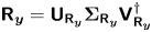 $\boldsymbol{\mathsf{R}}_{\boldsymbol {y}} = {\boldsymbol{\mathsf{U}}}_{\boldsymbol{\mathsf{R}}_{\boldsymbol {y}} } \boldsymbol {\Sigma }_{\boldsymbol{\mathsf{R}}_{\boldsymbol {y}} } {\boldsymbol{\mathsf{V}}}_{\boldsymbol{\mathsf{R}}_{\boldsymbol {y}} }^{\dagger }$ is the singular value decomposition of
 $\boldsymbol{\mathsf{R}}_{\boldsymbol {y}}$, such that
 ${\boldsymbol {\Sigma }}_{\boldsymbol{\mathsf{R}}_{\boldsymbol {y}} }$ is a diagonal matrix with elements
 $\sigma _i$, and
 ${\boldsymbol{\mathsf{U}}}_{\boldsymbol{\mathsf{R}}_{\boldsymbol {y}} }$ and
 ${\boldsymbol{\mathsf{V}}}_{\boldsymbol{\mathsf{R}}_{\boldsymbol {y}} }$ are unitary matrices describing forcing and response spaces, respectively. The matrix
 ${\boldsymbol {\Sigma }}_{\skew4\hat {\boldsymbol{\mathsf{T}}}_{\boldsymbol {f}}}$ is also diagonal, with elements
 ${\sigma _i}/({\sigma _i^{2}+\epsilon })$. In the limit of vanishing noise,
 \begin{equation} \lim_{\epsilon\to 0} \dfrac{\sigma_i}{\sigma_i^{2}+\epsilon} = \begin{cases} \dfrac{1}{\sigma_i}, & \sigma_i \neq 0, \\ 0, & \sigma_i = 0, \end{cases} \end{equation}
and, thus,
 \begin{equation}\lim_{\epsilon\to 0} \skew3\hat{\boldsymbol{\mathsf{T}}}_{\boldsymbol{f}} = \text{pinv}\left({\boldsymbol{\mathsf{R}}_{\boldsymbol{y}} }\right), \quad \lim_{\epsilon\to 0} \skew3\hat{\boldsymbol{\mathsf{T}}}_{\boldsymbol{u}}= \boldsymbol{\mathsf{R}}\boldsymbol{\mathsf{B}}\text{pinv}\left({\boldsymbol{\mathsf{R}}_{\boldsymbol{y}} }\right), \end{equation}
recovering the method proposed by Towne etal. (Reference Towne, Lozano-Durán and Yang2020). As the Moore–Penrose pseudo-inverse is equivalent to a least-square solution of a linear system (Lanczos Reference Lanczos1997, pp. 124–127), the estimated force can be understood as the minimum-norm force that generates a sensor reading. These results can be generalized to cases with a generic force CSD, where
 \begin{equation} \skew4\hat{\boldsymbol{\mathsf{T}}}_{\boldsymbol{f}} = \lim_{\epsilon\to 0} \skew4\hat{\boldsymbol{\mathsf{F}}}\boldsymbol{\mathsf{R}}_{\boldsymbol{y}}^{\dagger} (\boldsymbol{\mathsf{R}}_{\boldsymbol{y}}\skew4\hat{\boldsymbol{\mathsf{F}}}\boldsymbol{\mathsf{R}}_{\boldsymbol{y}}^{\dagger}+\epsilon\boldsymbol{\mathsf{I}})^{-1} = \skew2\hat{\boldsymbol{\mathsf{F}}}^{1/2} \text{pinv}\left({\boldsymbol{\mathsf{R}}_{\boldsymbol{y}}\skew2\hat{\boldsymbol{\mathsf{F}}}^{1/2}}\right). \end{equation}
A least-square estimation, using  $\skew2\hat {\boldsymbol{\mathsf{F}}}^{-1}$ as metric, is obtained. Expected force components are favoured by the estimation.
We illustrate the trend with a simple model, with two force components and one sensor, and CSDs given by
 \begin{equation}\boldsymbol{\mathsf{R}}_{\boldsymbol{y}} = \left[ \begin{matrix} 1 & 1 \end{matrix}\right],\quad \skew4\hat{\boldsymbol{\mathsf{F}}} = \left[ \begin{matrix} 1 & 0 \\ 0 & \gamma \end{matrix}\right],\quad \text{and}\quad \skew2\hat{\boldsymbol{\mathsf{N}}} = \left[ \begin{matrix} \epsilon \end{matrix}\right]. \end{equation}
Taking the limit  $\epsilon \to 0$,
 \begin{equation} \skew4\hat{\boldsymbol{\mathsf{T}}}_{\boldsymbol{f}} = \lim_{\epsilon\to 0} \frac{1} {1+\gamma+\epsilon} \left[ \begin{matrix} 1 \\ \gamma \end{matrix}\right] = \left[ \begin{matrix} \dfrac{1} {1+\gamma} \\ \dfrac{\gamma} {1+\gamma} \end{matrix}\right]. \end{equation}
If the second force component is expected to be small,  $\gamma \ll 1$, the estimated force is dominated by the first component. In the opposite scenario,
 $\gamma \gg 1$, the second component dominates the estimation.
For non-zero noise,  $\epsilon > 0$, a reduction in the estimation efficiency is expected. For the same readings, larger
 $\epsilon$ leads to smaller estimated force components, as is seen by inspection of
 $\boldsymbol {\Sigma }_{\boldsymbol{\mathsf{R}}_{\boldsymbol {y}}}$. Separating sensor readings into a noiseless component (
 $\boldsymbol {y}_0$) and a noise component (
 $\boldsymbol {n}$) such that
 $\hat {\boldsymbol {y}} = \hat {\boldsymbol {y}}_{0} + \hat {\boldsymbol {n}}$, the sensor CSD (
 $\skew3\hat {\boldsymbol{\mathsf{Y}}} = \langle \hat {\boldsymbol {y}}\hat {\boldsymbol {y}}^{\dagger }\rangle$) can be written as
 $\skew3\hat {\boldsymbol{\mathsf{Y}}} = \skew3\hat {\boldsymbol{\mathsf{Y}}}_0 + \hat {\epsilon } \boldsymbol{\mathsf{I}}$. The CSD of the estimated sensor reading is given by
 \begin{align} \skew3\hat{\skew3\tilde{\boldsymbol{\mathsf{Y}}}} &= \boldsymbol{\mathsf{C}}\hat{\boldsymbol{\mathsf{T}}_{\boldsymbol{u}}} \skew3\hat{\boldsymbol{\mathsf{Y}}} \boldsymbol{\mathsf{T}}_{\boldsymbol{u}}^{\dagger}\boldsymbol{\mathsf{C}}^{\,\dagger},\nonumber\\ &= \boldsymbol{\mathsf{R}}_{\boldsymbol{y}} \boldsymbol{\mathsf{R}}_{\boldsymbol{y}}^{\dagger}\left( \boldsymbol{\mathsf{R}}_{\boldsymbol{y}} \boldsymbol{\mathsf{R}}_{\boldsymbol{y}} ^{\,\dagger} +\epsilon \boldsymbol{\mathsf{I}} \right)^{-1} \left(\skew3\hat{\boldsymbol{\mathsf{Y}}}_0 +\epsilon \boldsymbol{\mathsf{I}} \right) \left( \boldsymbol{\mathsf{R}}_{\boldsymbol{y}} \boldsymbol{\mathsf{R}}_{\boldsymbol{y}} ^{\,\dagger} +\epsilon \boldsymbol{\mathsf{I}} \right)^{-1}\boldsymbol{\mathsf{R}}_{\boldsymbol{y}} \boldsymbol{\mathsf{R}}_{\boldsymbol{y}}^{\dagger}. \end{align}
By inspection it can be seen that the noiseless reading is only recovered for  $\epsilon \to 0$. Using
 $\skew3\hat {\boldsymbol{\mathsf{F}}} = \boldsymbol{\mathsf{I}}$, the expected sensor CSD is given by
 $\skew3\hat {\boldsymbol{\mathsf{Y}}}_0 = \boldsymbol{\mathsf{R}}_{\boldsymbol {y}} \boldsymbol{\mathsf{R}}_{\boldsymbol {y}}^{\dagger } = {\boldsymbol{\mathsf{U}}}_{\boldsymbol{\mathsf{R}}_{\boldsymbol {y}} } \boldsymbol {\Sigma }_{\boldsymbol{\mathsf{R}}_{\boldsymbol {y}} }^{2} {\boldsymbol{\mathsf{U}}}_{\boldsymbol{\mathsf{R}}_{\boldsymbol {y}} }^{\dagger }$, and (2.29) becomes
 \begin{equation} \skew3\hat{\skew3\tilde{\boldsymbol{\mathsf{Y}}}} = \boldsymbol{\mathsf{R}}_{\boldsymbol{y}} \boldsymbol{\mathsf{R}}_{\boldsymbol{y}}^{\dagger} \left( \boldsymbol{\mathsf{R}}_{\boldsymbol{y}} \boldsymbol{\mathsf{R}}_{\boldsymbol{y}} ^{\,\dagger} +\epsilon \boldsymbol{\mathsf{I}} \right)^{-1}\boldsymbol{\mathsf{R}}_{\boldsymbol{y}} \boldsymbol{\mathsf{R}}_{\boldsymbol{y}}^{\dagger} = {\boldsymbol{\mathsf{U}}}_{\boldsymbol{\mathsf{R}}_{\boldsymbol{y}} } \boldsymbol{\Sigma}_{\boldsymbol{\mathsf{R}}_{\boldsymbol{y}} }^{4} \left( \boldsymbol{\Sigma}_{\boldsymbol{\mathsf{R}}_{\boldsymbol{y}} }^{2} + \epsilon \boldsymbol{\mathsf{I}} \right)^{-1} {\boldsymbol{\mathsf{U}}}_{\boldsymbol{\mathsf{R}}_{\boldsymbol{y}} }^{\dagger}, \end{equation}
showing that for finite-noise levels the sensor CSD is underestimated.
2.4. Matrix-free approach
The simplest method for obtaining the resolvent-based estimator described above involves matrix inversion, followed by direct application of (2.18) and (2.22). The approach thus becomes prohibitively expensive for large matrices. Matrix inversion can be avoided by solution of the linear system
 \begin{equation} ( -\mathrm{i} \omega \boldsymbol{\mathsf{I}} - \boldsymbol{\mathsf{A}}) \hat{\boldsymbol{u}} = \boldsymbol{\mathsf{B}} \skew2\hat{\boldsymbol{f}}, \end{equation}
as done by Schmidt etal. (Reference Schmidt, Towne, Rigas, Colonius and Brès2018). Although less demanding, computational cost typically limits this approach to two-dimensional problems. Time-marching schemes have been used by Tam & Pastouchenko (Reference Tam and Pastouchenko2002), in which individual rows of  $\boldsymbol{\mathsf{R}}_{\boldsymbol {y}}$ are obtained via integration of harmonically forced adjoint equations; the approach is applicable for much larger systems. Repeating the procedure for different frequencies and sensors, an estimation based on (2.9), (2.21) and (2.22) can be obtained. Here we propose a method that significantly further reduces computational cost, providing solutions for all frequencies with a single time-march. This is achieved by integration of the direct and adjoint equations, similar to what is done in other matrix-free approaches (Semeraro etal. Reference Semeraro, Pralits, Rowley and Henningson2013).
For simplicity, we assume that  $\boldsymbol{\mathsf{F}}(t)=\boldsymbol{\mathsf{I}}\delta (t)$,
 $\boldsymbol{\mathsf{B}}=\boldsymbol{\mathsf{I}}$ and
 $\boldsymbol{\mathsf{N}}(t)=\epsilon \boldsymbol{\mathsf{I}}\delta (t)$.
Consider the system
 \begin{equation} -\dfrac{\textrm{d}\boldsymbol{w}_i}{\textrm{d}t} = \boldsymbol{\mathsf{A}}^{\dagger} \boldsymbol{w}_i + \boldsymbol{\mathsf{C}}_i^{\dagger} \delta(t), \end{equation}
with a null terminal condition, and where  $\boldsymbol{\mathsf{A}}^{\dagger }$ corresponds to the adjoint linearised Navier–Stokes operator and
 $\boldsymbol{\mathsf{C}}_i^{\dagger }$ is the
 $i$th column of the adjoint of
 $\boldsymbol{\mathsf{C}}$. The impulse response of (2.32) can be replaced by a terminal condition,
 $\boldsymbol {w}_i(0) = \boldsymbol{\mathsf{C}}_i^{\dagger }$. Taking the Fourier transform of (2.32) leads to
 \begin{equation} ({\rm i}\omega\boldsymbol{\mathsf{I}} - \boldsymbol{\mathsf{A}}^{\dagger} ) \hat{\boldsymbol{w}}_i = \boldsymbol{\mathsf{C}}_i^{\dagger} \end{equation}
and, thus,
 \begin{equation} \hat{\boldsymbol{w}}_i = \boldsymbol{\mathsf{R}}^{\,\dagger} \boldsymbol{\mathsf{C}}_i^{\dagger}. \end{equation}
The  $i$th component of
 $\boldsymbol{\mathsf{R}}_{\boldsymbol {y}}^{\dagger }$, given by
 $\boldsymbol{\mathsf{R}}^{\,\dagger }\boldsymbol{\mathsf{C}}_i^{\dagger }$, is the Fourier transform of the response of (2.32). The resolvent can thus be constructed row-by-row as
 \begin{equation} \hat{\boldsymbol{\mathsf{R}}_{\boldsymbol{y}}} (\omega) = \left[ \begin{matrix} - & \hat{\boldsymbol{w}}_1^{\dagger}(\omega) & - \\ - & \hat{\boldsymbol{w}}_2^{\dagger}(\omega) & - \\ & \vdots & \end{matrix} \right]. \end{equation}
The values of  $\boldsymbol {w}_i(-t)$ are the sensitivities of the
 $i$th measurement at time
 $t=0$ to forces at the instant
 $-t$; in the frequency domain the same information is contained in
 $\hat {\boldsymbol {w}}_i(\omega )$.
From solutions of the equation
 \begin{equation} \dfrac{\textrm{d}\boldsymbol{q}_i}{\textrm{d}t} = \boldsymbol{\mathsf{A}} \boldsymbol{q}_i + \boldsymbol{w}_i(t), \end{equation}
which has frequency domain representation
 \begin{equation} (-\textrm{i}\omega\boldsymbol{\mathsf{I}} - \boldsymbol{\mathsf{A}}) \hat{\boldsymbol{q}}_i = \hat{\boldsymbol{w}}_i \end{equation}
and, thus,
 \begin{equation} \hat{\boldsymbol{q}}_i = \boldsymbol{\mathsf{R}} \hat{\boldsymbol{w}}_i, \end{equation}
the operator  $\boldsymbol{\mathsf{R}}\boldsymbol{\mathsf{R}}_{\boldsymbol {y}}^{\dagger }$ can be constructed from Fourier transforms of the solutions as
 \begin{equation} \boldsymbol{\mathsf{R}} \boldsymbol{\mathsf{R}}_{\boldsymbol{y}}^{\dagger} (\omega) = \boldsymbol{\mathsf{R}} \left[ \begin{matrix} | & |& \\ \hat{\boldsymbol{w}}_1(\omega) & \hat{\boldsymbol{w}}_2(\omega) & \cdots \\ | & |& \end{matrix} \right] = \left[ \begin{matrix} | & |& \\ \hat{\boldsymbol{q}}_1(\omega) & \hat{\boldsymbol{q}}_2(\omega) & \cdots \\ | & |& \end{matrix} \right]. \end{equation}
As
 \begin{equation} \boldsymbol{\mathsf{R}}_{\boldsymbol{y}} \boldsymbol{\mathsf{R}}_{\boldsymbol{y}}^{\dagger}= \boldsymbol{\mathsf{C}}\boldsymbol{\mathsf{R}} \boldsymbol{\mathsf{R}}_{\boldsymbol{y}}^{\dagger}, \end{equation}
this term can be obtained from observations of the system  $\hat {\boldsymbol {y}}_i = \boldsymbol{\mathsf{C}} \hat {\boldsymbol {q}}_i$. State and force estimation functions,
 \begin{equation} \skew4\hat{\boldsymbol{\mathsf{T}}}_{\boldsymbol{u}} = \boldsymbol{\mathsf{R}} \boldsymbol{\mathsf{R}}_{\boldsymbol{y}} ^{\,\dagger} \left( \boldsymbol{\mathsf{R}}_{\boldsymbol{y}} \boldsymbol{\mathsf{R}}_{\boldsymbol{y}} ^{\,\dagger} + \epsilon \boldsymbol{\mathsf{I}} \right)^{-1}, \quad \skew4\hat{\boldsymbol{\mathsf{T}}}_{\boldsymbol{f}} = \boldsymbol{\mathsf{R}}_{\boldsymbol{y}} ^{\,\dagger} \left( \boldsymbol{\mathsf{R}}_{\boldsymbol{y}} \boldsymbol{\mathsf{R}}_{\boldsymbol{y}} ^{\,\dagger} + \epsilon \boldsymbol{\mathsf{I}} \right)^{-1}, \end{equation}
can then be constructed.
The procedure can be summarised in the following steps.
(i) Adjoint run: (2.32) is integrated for each sensor. Snapshots are saved on disk for later use.
(ii) Direct run: (2.35) is integrated for each sensor, with snapshots from the adjoint run loaded and interpolated at each time step, to provide the force term. The readings at the sensors and some other points of interest are calculated at each time step and saved separately.
Although the term  $\boldsymbol{\mathsf{R}}_{\boldsymbol {y}}\boldsymbol{\mathsf{R}}_{\boldsymbol {y}}^{\dagger }$ from (2.37) and (2.38) can be computed from flow snapshots of the direct run, saving sensor readings at each simulation time step is computationally cheap, and provides extra accuracy with negligible extra cost. Generalisation for any
 $\boldsymbol{\mathsf{B}}$ and
 $\boldsymbol{\mathsf{F}}$ is obtained by multiplying
 $\hat {\boldsymbol {w}}_i$ by
 $\boldsymbol{\mathsf{B}} \skew3\hat {\boldsymbol{\mathsf{F}}} \boldsymbol{\mathsf{B}}^{\dagger }$ prior to the integration of (2.35).
3. Comparison between causal and non-causal estimation
3.1. Model problem
We compare resolvent-based estimation (non-causal) and Kalman-filter estimation (causal) on a complex-valued linearised Ginzburg–Landau (GL) model, which is frequently used as a simple model that qualitatively mimics the behaviour of complex flows (Chomaz, Huerre & Redekopp Reference Chomaz, Huerre and Redekopp1991; Couairon & Chomaz Reference Couairon and Chomaz1999; Bagheri etal. Reference Bagheri, Henningson, Hœpffner and Schmid2009; Cavalieri etal. Reference Cavalieri, Jordan and Lesshafft2019; Towne etal. Reference Towne, Lozano-Durán and Yang2020), and, thus, constitutes a convenient benchmark. The comparison provides insights on advantages of using non-causal estimation tools when the necessary information for such is available.
The model takes the form
 \begin{equation} \frac{\partial \boldsymbol{u}(x,t)}{\partial t} = \boldsymbol{\mathsf{A}} \boldsymbol{u}(x,t) + \boldsymbol{f}(x,t), \quad \boldsymbol{\mathsf{A}} = - U \frac{\partial }{\partial x} + \mu(x) + \gamma \frac{\partial^{2} }{\partial x^{2}}, \end{equation}
and we use the parameters:  $U=6$,
 $\gamma =1-\mathrm {i}$ and
 $\mu (x)=\beta \mu _c(1-x/20)$, where
 $\mu _c=U^{2}\, {\rm Re} (\gamma)/|\gamma |^{2}$ is the critical value for onset of absolute instability (Bagheri etal. Reference Bagheri, Henningson, Hœpffner and Schmid2009). The parameters are similar to those used by Lesshafft (Reference Lesshafft2018). The terms in
 $\boldsymbol{\mathsf{A}}$ correspond to advection, growth/decay and diffusion, respectively. Dirichlet boundary conditions are considered at
 $x=0$ and
 $40$,
 $\boldsymbol {u}(0,t)=\boldsymbol {u}(40,t)=0$, and the initial condition
 $\boldsymbol {u}(x,0)=0$ is used. We consider a system with
 $\beta = 0.1$, leading to a moderate gain separation between optimal and suboptimal modes.
System observations are given by
 \begin{equation} \boldsymbol{y}(t) = \boldsymbol{\mathsf{C}} \boldsymbol{u}(x,t), \end{equation}
where the operator  $\boldsymbol{\mathsf{C}}$ imposes Gaussian-shaped sensors:
 $\boldsymbol{\mathsf{C}}$ is defined such that the
 $i$th entry of
 $\boldsymbol {y}(t)$ is
 \begin{equation} \boldsymbol{y}_i(t) = \frac{1} {\sqrt{2\pi\sigma_c^{2}}} \int \textrm{exp}{({-(x-x_i)^{2}}/{2\sigma_{c}^{2}})} \boldsymbol{u}(x,t)\,\textrm{d}x, \end{equation}
with  $\sigma _c=0.5$. The number and positions of sensors (
 $x_i$) will be indicated for each case we consider.
The spatial domain is discretised using a second-order upwind differentiation scheme at points evenly distributed between  $x=0$ and
 $40$, with
 ${\rm \Delta} x=0.1$, and the system is time integrated from
 $t=0$ to
 $t=500$ with a Crank–Nicolson scheme with time step,
 ${\rm \Delta} t = 10^{-2}$.
For application to a turbulent flow, the force term,  $\boldsymbol {f}(x,t)$, would represent nonlinear interactions contained in the nonlinear advection term of the Navier–Stokes equations (McKeon & Sharma Reference McKeon and Sharma2010). Various assumptions will be made regarding the statistics of this term. We first consider
 $\boldsymbol {f}(x,t)$ to be spatially and temporally white. With the parameters cited above,
 $\boldsymbol{\mathsf{A}}$ is globally stable; it is locally convectively unstable in the first part of the domain (
 $x<20$), and locally convectively stable in the second part (
 $x>20$). A realisation of the system response to spatiotemporally white forcing is shown in figure 2.
Sample of the response of the GL model under white noise forcing. Colour scale corresponds to responses real part. The growth of perturbations for  $x<20$, their decay for
 $x>20$, and the convection behaviour of the model can be observed.

System gains are shown in figure 3. Optimal force and response modes for the full-rank system are shown in figure 4. The force modes observable by two sensors, and their corresponding responses, are shown in figure 5. We note that forces observable by different sensors, although linearly independent, can be quite similar: this is typically the case when the system has large gain separations. In this scenario, the extra information that can be obtained by adding a given sensor is more clearly visualised by plotting an orthogonal basis for the observable space: i.e. the component of the newly added observable force that is orthogonal to the previous observable space.
Gains on the GL model.

Ginzburg–Landau response ( $a$) and force (
 $b$) modes. From top to bottom are the optimal and first two suboptimal modes. Solid lines correspond to the amplitude envelope and dashed lines show the real part.

Observable forces ( $\boldsymbol{\mathsf{R}}_{\boldsymbol {y}}^{\dagger } \boldsymbol{\mathsf{C}}^{\,\dagger }$ and their corresponding excited responses
 $\boldsymbol{\mathsf{R}}\boldsymbol{\mathsf{R}}_{\boldsymbol {y}}^{\dagger } \boldsymbol{\mathsf{C}}^{\,\dagger }$) for two Gaussian sensors at
 $x=10$ (blue) and
 $30$ (red). Solid and dotted lines correspond to the amplitude envelope and real part, the dashed back lines indicate sensor positions. On the right, observable forces and responses are made orthogonal.

Figure 6 compares Kalman-filter and resolvent-based estimations for  $\boldsymbol {u}(10,t)$ and
 $\boldsymbol {u}(30,t)$ using one sensor at
 $x=20$. Force estimation from the Kalman filter were obtained using the estimated state in (2.1). Alternatively, they can be estimated using the frequency-domain counterpart of (2.1); in that case, it is necessary to account for windowing effects. This can be accomplished by multiplying (2.1) by a window function
 $w(t)$ and manipulation of the terms, leading to
 \begin{equation} \dfrac{\textrm{d}(w\boldsymbol{u})}{\textrm{d}t}(t) = \boldsymbol{\mathsf{A}} (w\boldsymbol{u})(t) + \boldsymbol{\mathsf{B}} (w\boldsymbol{f})(t) + \dfrac{\textrm{d}w}{\textrm{d}t}(t) \boldsymbol{u}(t), \end{equation}
with frequency-domain representation given by
 \begin{equation} \overline{\boldsymbol{u}}(\omega) = \boldsymbol{\mathsf{R}} \left(\boldsymbol{\mathsf{B}} \overline{\boldsymbol{f}}(\omega) + \overline{\boldsymbol{u}}'(\omega) \right), \end{equation}
where
 \begin{equation} \overline{\boldsymbol{u}} (\omega) = \int_{-\infty}^{\infty} w(t)\boldsymbol{u}(t) \mathrm{e}^{ {\mathrm{i}} \omega t}\,\textrm{d}t, \quad \overline{\boldsymbol{u}}' (\omega) = \int_{-\infty}^{\infty} \frac{\textrm{d}w}{\textrm{d}t}(t)\boldsymbol{u}(t) \mathrm{e}^{ {\mathrm{i}} \omega t}\,\textrm{d}t \end{equation}
are respectively the estimation of  $\hat {u}(\omega )$ using a window
 $w(t)$, and an associated force correction term that must be included to account for the window function. The method is described in detail by Martini etal. (Reference Martini, Cavalieri, Jordan and Lesshafft2019), with a discussion of the impact of window choice on the accuracy for a given sampling rate.
Comparison between resolvent and Kalman-filter methods for state estimation with one sensor.

The Kalman-filter and resolvent-based estimations provide identical results for the downstream position, but only the resolvent-based estimation can estimate the upstream position,  $x=10$. Figure 7 compares root-mean-square (r.m.s.) errors of both methods for different sensor configurations. Both methods show the same error downstream of the last sensor, with the resolvent method consistently showing smaller errors in other regions.
Comparison between resolvent and Kalman-filter methods for states estimation with one, three and five sensors, indicated by vertical dotted lines. The dashed black line represents state r.m.s. on each position. Root-mean-square errors on each point are normalized by the global error r.m.s.

Two-point state correlations were constructed from the original and estimated systems. As seen in figure 8, the resolvent-based estimation requires a smaller number of sensors for an accurate estimation of two-point state statistics. Being smoother, responses are easier to estimate than forces, which, being white in space, are difficult to represent with a small number of force modes.
Response and force two-point correlations for zero time-lag, obtained using the raw data (left most), Kalman-filter and resolvent-based estimations. Colour scale indicates the absolute level, normalized by the maximum value found on the raw data. White markers indicate the sensor position. ( $a$) Response two-point correlations. (
 $b$) Force two-point correlations.

Cross-spectral density estimates were obtained for both forcing and state via the Welch (Reference Welch1967) method, with a window length of 40 % and 80 % overlap. Comparison of CSDs obtained with the original signal and results from Kalman-filter and resolvent-based estimations are shown in figure 9. Results again show that the resolvent-based approach leads to a more accurate CSD estimation for a given number of sensors. For cases with small numbers of sensors, it becomes clear that measurements may be used to estimate upstream information, which is not possible using a Kalman filter. Furthermore, the resolvent-based approach provides a faster convergence of both force and response estimations.
Same as figure 8 for CSD at  $\omega =1$. (
 $a$) Response CSD. (
 $b$) Force CSD.

3.2. Estimation of a system driven by coloured forcing
To assess the robustness of resolvent-based estimation when exact knowledge of force statistics is not available a priori, we construct resolvent-based and Kalman-filter estimators based on an assumption of spatiotemporally white forcing, and use these to estimate a system driven by coloured forces. We consider a forcing cross-spectral density model given by
 \begin{equation} \left\langle\,\skew2\hat{\boldsymbol{f}}(x_1,\omega) \skew2\hat{\boldsymbol{f}} (x_2,\omega)\right\rangle =
{\rm e}^{{\rm i}k_h(x_2-x_1)}{\rm e}^{-({(x_1-x_2)^{2}}/{L_c^{2}})}{\rm e}^{-({(x_1-x_c(\omega))^{2}}/{L^{2}})}
{\rm e}^{-({(x_2-x_c(\omega))^{2}}/{L^{2}})} + {\rm c.c.}, \end{equation}
where  $\langle \cdot \rangle$ represents an ensemble average. The first term creates wave-like behaviour, the second imposes a coherence length and the two final terms define an amplitude envelope (Cavalieri etal. Reference Cavalieri, Jordan and Lesshafft2019). The following parameters were used:
 $k_h = 0.42$,
 $L=4$,
 $L_c=5$ and
 $x_c(\omega ) = 25-5|\omega |$.
Estimation is performed under the assumption that  $\boldsymbol{\mathsf{F}}(t)=\boldsymbol{\mathsf{I}}\delta (t)$. Results for vanishing sensor noise are presented in figures 10 and 11. The method is capable of distinguishing the CSD for different frequencies, despite the underlying assumption of white forcing.
Same as figure 8 for frequency-dependent CSDs. Estimation for  $\omega =1$. (
 $a$)Response CSD. (
 $b$) Force CSD.

Same as figure 8 for frequency-dependent CSDs. Estimation for  $\omega =3$. (
 $a$)Response CSD. (
 $b$) Force CSD.

If, on the other hand, information is available concerning the force statistics, this can be used to improve the estimation performance. We illustrate this case using a rank-2 force CSD, constructed as
 \begin{gather} \langle\,\skew2\hat{\boldsymbol{f}}(x_1,\omega) \skew2\hat{\boldsymbol{f}} (x_2,\omega)\rangle = \boldsymbol{f}_1\ \boldsymbol{f}_1^{\dagger} + \boldsymbol{f}_2\ \boldsymbol{f}_2^{\dagger}, \end{gather}
 \begin{gather} \boldsymbol{f}_1(x) = e^{ -(x-5)^{2}}+e^{ -(x-35)^{2}}, \end{gather}
 \begin{gather} \boldsymbol{f}_2(x) = e^{ -(x-15)^{2}}+e^{ -(x-25)^{2}}. \end{gather}
This produces forces at  $x=5$ that are perfectly correlated with forces at
 $x=35$, and likewise for positions
 $15$ and
 $25$. Figure 12 compares resolvent-based estimations obtained using the white force assumption to those obtained using the real force CSD. Use of the correct force CSD leads to a substantial improvement in the estimation of both response and force when a single sensor is used, and an exact estimation when two sensors are used, as a result of the very low rank of the force considered.
Same as figure 8, comparing estimation with the assumption of white-noise forcing, and using the correct underlining force CSDs. Estimation for  $\omega =3$. (
 $a$) Response CSD. (
 $b$) Force CSD.

Although observable forces for this system are always upstream of the sensors, downstream forces are correlated with observable forces: these forces, and their responses are thus correctly estimated.
3.3. Resolvent-based estimation as an alternative to the Kalman filter
Towne etal. (Reference Towne, Lozano-Durán and Yang2020) suggested that resolvent-based estimation can provide a departure point for the control of complex turbulent flows. But real-time control requires causal estimation. We therefore consider a truncation of the kernel of the resolvent-based estimator to is causal component (Sasaki etal. Reference Sasaki, Tissot, Cavalieri, Silvestre, Jordan and Biau2016), and we compare this to kernels obtained using the standard Kalman filter.
The comparisons of figure 6 suggest that Kalman-filter and resolvent-based estimators may be equivalent at positions downstream of the sensor. This is an interesting possibility, as the Kalman filter is a central feature of LQG control methods. If the methods are indeed equivalent when the resolvent-based estimator is truncated to its causal component, then its low cost would enable extension of LQG methods to large systems. We proceed by comparing the kernels obtained for the two methods.
The resolvent-based kernel is obtained by converting the resolvent-based estimation function to the time domain by inverse Fourier transform of (2.22). A state estimation is then obtained via convolution of the kernel,  ${\boldsymbol{\mathsf{T}}}_{\boldsymbol {u}}$, and readings,
 $\boldsymbol {y}(t)$, i.e.
 \begin{equation} \boldsymbol{u}(t) = \int_{-\infty}^{\infty} \boldsymbol{\mathsf{T}}_{\boldsymbol{u}} (\tau) \boldsymbol{y}(t-\tau) \,\textrm{d} \tau, \end{equation}
where 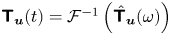 ${\boldsymbol{\mathsf{T}}}_{\boldsymbol {u}} (t) = \mathcal {F}^{-1}\left ({ \skew4\hat {\boldsymbol{\mathsf{T}}}_{\boldsymbol {u}}} (\omega ) \right )$ (Sasaki etal. Reference Sasaki, Tissot, Cavalieri, Silvestre, Jordan and Biau2016). The Kalman-filter estimation is obtained via integration of
 \begin{equation} \dfrac{\textrm{d}\tilde{\boldsymbol{u}}}{\textrm{d}t} = \boldsymbol{\mathsf{A}} \tilde{\boldsymbol{u}} + \boldsymbol{\mathsf{L}}(\boldsymbol{y}-\boldsymbol{\mathsf{C}} \tilde{\boldsymbol{u}}), \end{equation}
where  $\boldsymbol{\mathsf{L}}$ is the Kalman gain. A formal solution is
 \begin{equation} \tilde{\boldsymbol{u}}(t) = \int_{-\infty}^{t} \mathrm{e}^{\left(\boldsymbol{\mathsf{A}}-\boldsymbol{\mathsf{L}}\boldsymbol{\mathsf{C}}\right)(t-\tau)} \boldsymbol{\mathsf{L}} \boldsymbol{y}(\tau) \,\textrm{d} \tau = \int_{-\infty}^{\infty} \boldsymbol{\mathsf{T}}_{\boldsymbol{u}}^{kal}(\tau) \boldsymbol{y}(t-\tau) \,\textrm{d} \tau, \end{equation}
where
 \begin{equation} \boldsymbol{\mathsf{T}}_{\boldsymbol{u}}^{kal}(t) = \begin{cases} \mathrm{e}^{\left(\boldsymbol{\mathsf{A}}-\boldsymbol{\mathsf{L}}\boldsymbol{\mathsf{C}}\right)t} \boldsymbol{\mathsf{L}}, & t \ge 0, \\ 0, & t < 0, \end{cases} \end{equation}
is the Kalman-filter kernel.
The kernels,  ${\boldsymbol{\mathsf{T}}}_{\boldsymbol {u}}$ and
 ${\boldsymbol{\mathsf{T}}}_{\boldsymbol {u}}^{kal}$, are compared using different sensor configurations. Three probes, at locations
 $x=5,20$ and
 $35$, referred to as
 $z_1$,
 $z_2$ and
 $z_3$, are used. Figure 13 shows kernels constructed using one sensor. The Kalman-filter kernel for probe
 $z_3$ exactly reproduces the resolvent-based kernel for all values of sensor noise, and the causal part of the resolvent-based kernel closely approximates that of the Kalman filter for the probe
 $z_2$. While the Kalman filter makes no estimation on the probe
 $z_1$, the resolvent-based estimation provides a non-causal estimation.
Comparison between resolvent estimation (solid lines) and Kalman-filter estimation (dashed lines) kernels using one sensor for different values of sensor noise  $\epsilon$. Blue, red and yellow lines indicate kernels for probes
 $z_1$,
 $z_2$ and
 $z_3$, respectively. Sensor and probes locations are shown on the bottom. In the legend,
 $\mathcal {T}_{u,y_i,z_j}$, corresponds to the transfer function term to be convoluted with the
 $i$th sensor for obtaining estimates at the
 $j$th probe.

The match between the causal component of the resolvent-based kernel and that of the Kalman filter reinforces the idea that the latter can be obtained via a truncation of the resolvent-based kernel. This is in accordance with the results obtained by Fraser & Potter (Reference Fraser and Potter1969): an optimal non-causal (smoothing) estimation is equivalent to the combination of a pair of Kalman filters, one moving forward and the other backward in time; in systems where no information can be gained from the backward-directed filter, the optimal causal and non-causal estimates coincide.
Figure 14 shows the kernels obtained with inclusion of an additional upstream sensor. The kernels are similar for probes  $z_2$ and
 $z_3$. However, the resolvent-based kernel for probe
 $z_1$ has causal contributions from sensor
 $y_1$ and non-causal contributions from sensor
 $y_2$; and, as suggested by the foregoing argument, resolvent-based and Kalman-filter kernels do not match. Addition of a further downstream sensor leads to kernels that differ for all probe locations, as shown in figure 15.
Same as figure 13 using two sensors, with sensor noise of  $\epsilon =10^{-2}$.

Same as figure 13 using three sensors, with sensor noise of  $\epsilon =10^{-2}$.

When the methods are not equivalent, we note that the resolvent-based kernel is consistently lower than those of the Kalman filter. Truncation of the former to its causal components will thus lead to an underestimation. This can also be interpreted in terms of the results of Fraser & Potter (Reference Fraser and Potter1969): as the non-causal estimation is the average of the forward- and backward-moving Kalman filters, truncating the resolvent-based kernel to its causal part corresponds to a zeroing of the backward-directed filter, leading to an underestimation.
The dominance of the downstream-travelling mode in the present model makes it easy to identify sensor locations which will produce predominantly causal resolvent-based kernels, and from which Kalman-filter estimation can be obtained. Many fluid flows of interest are dominated by downstream-travelling modes (incompressible boundary layers and jets, see Beneddine etal. (Reference Beneddine, Yegavian, Sipp and Leclaire2017); Sasaki etal. (Reference Sasaki, Piantanida, Cavalieri and Jordan2017b) for examples) and may therefore be amenable to the obtention of a Kalman-filter estimator, using the resolvent-based approach we describe, at substantially lower computational cost and without requiring the construction of a reduced-order model. In more complex systems, where upstream- and downstream-travelling modes may be relevant, the procedure is not necessarily simple, or possible. In such cases optimal non-causal kernels can be converted to optimal causal kernels by solving associated Wiener–Hopf equations (Martinelli Reference Martinelli2009). Such equations are, however, not easily solved if more than one sensor is used.
3.4. Comparison with truncated response-mode estimation
The recognition that large resolvent gain separation implies that the response of a system may be relatively insensitive to the specific details of its underlying driving forces (McKeon & Sharma Reference McKeon and Sharma2010) has motivated several studies (Gomez Carrasco etal. Reference Gomez Carrasco, Blackburn, Rudman, Sharma and McKeon2014; Beneddine etal. Reference Beneddine, Yegavian, Sipp and Leclaire2017; Symon etal. Reference Symon, Dovetta, McKeon, Sipp and Schmid2017) in which the system response is estimated using the dominant response modes. We refer to such approaches as truncated response-mode estimation (TRME). Response-mode amplitudes and phases are obtained by fitting them to available flow data. Parabolized stability equations (PSE) have also been used with the same underlying idea (Sasaki etal. Reference Sasaki, Piantanida, Cavalieri and Jordan2017b): these track the fastest growing perturbation, which often approximates the optimal resolvent response mode (Towne, Rigas & Colonius Reference Towne, Rigas and Colonius2019), and can therefore be understood as a rank-1 truncated response-mode estimation.
Beneddine etal. (Reference Beneddine, Yegavian, Sipp and Leclaire2017) showed that sensors for a jet need to be located in regions where the optimal modes have significant amplitude; with this choice of sensor location, flow quantities downstream were estimated. Although successful, the approach lacks a rigorous justification: it is not expected that such a basis will be optimal for any choice of sensors. The authors argue that sensors should be located around the peak of the response mode, which should lead to better signal-to-noise ratios. Our results suggest that such locations are indeed desirable, but with a slightly different interpretation: the observable force subspace for sensors at these locations has a larger projection of the optimal force mode. A rank-1 TRME was also used to improve a data assimilation of the flow around an airfoil by Symon (Reference Symon2018), but to the best of our knowledge higher-rank estimations were not attempted. In what follows we show that higher-order TRMEs are not suitable for estimation, and we provide an explanation as to why this is the case.
The orthogonality of the response-mode basis suggests that this constitutes an efficient basis if the projection is made using an  $L^{2}$ inner product. This norm can be emulated using many sensors uniformly distributed throughout the flow. Figure 16 compares errors associated with resolvent-based and truncated response-mode estimations when uniformly spaced sensors are used. For the latter, the number of response modes corresponds to the number of sensors. Response-truncation errors are always larger than the resolvent-based estimation, but the results are similar.
Comparisons between r.m.s. errors of resolvent-based estimations and TRME. Allcurves are normalised by the global r.m.s. error.

A different picture emerges when sensors are not uniformly spaced, but concentrated in the upstream region of the domain. Figure 17 shows that TRME errors are orders of magnitude larger than the proposed method. This is a consequence of an ill-posed fit of the optimal response mode basis to the collocation points used. From figure 4 we see that only the optimal force mode is biased towards the upstream flow region, suboptimal force modes being spread throughout the domain. As a sensor in a convection-dominated system can only observe forces upstream of its location, the use of upstream sensors to obtain forces spread throughout the domain leads to an ill-posed fitting. The resolvent-based estimation, on the other hand, focuses on the observable force subspace, thus providing a naturally stable method.
Comparisons between r.m.s. errors of resolvent-based and TRME methods with sensors located at an upstream region. All curves are normalised by the global r.m.s. error.

We illustrate the origin of the TRME ill-posed fitting with a simpler problem: curve fitting using polynomials, as shown in figure 18. Fittings were obtained using uniformly spaced collocation points, Gauss–Lobatto collocation points and collocation points located on a small domain. Even though all fits use the same basis, fit performances vary considerably: Gauss–Lobatto points provide uniform, exponential convergence (Trefethen Reference Trefethen2000); equispaced points provide non-uniform convergence; and localised collocation points lead to large errors, which increase with the polynomial order. This situation can be understood as analogous to that which underpins the results of figure 17, once it is realised that the procedure is implicitly trying to represent the systems forces with a particular choice of basis: force modes in the case of TRME and observable forces in the case of the resolvent-based method.
Fitting of a Gaussian curve using polynomials of orders 4 and 15, markers indicate the collocation points used. Collocation points are ( $a$) uniformly spaced on the first half of the domain, (
 $b$) uniformly spaced throughout the domain, (
 $c$) on Gauss–Lobatto points.

For estimation purposes, the instability of TRME may be worked around by using more sensors than response modes, leading to a least-square minimisation of the sensor errors, as was done by Gomez Carrasco etal. (Reference Gomez Carrasco, Blackburn, Rudman, Sharma and McKeon2014). The sensors should be weighted in order to reproduce an inner product for which the response modes are orthogonal. This approach, however, discards sensor information, which could be used for higher accuracy. It can be justified if resolvent modes are readily available, but if they need to be constructed by traditional methods, this would be more demanding than using the method we propose.
4. Application in transitional and turbulent flows
4.1. Transitional flat-plate boundary layer
We perform state-estimation in a two-dimensional spatially evolving transitional boundary layer, with Reynolds number  $Re=1000$ based on the displacement thickness at the beginning of the domain. The free stream velocity is taken as the reference value for non-dimensional quantities. The base flow, obtained from a Blasius boundary layer solution, is shown together with sensors and probes used in figure 19. The linearised Navier–Stokes equations are solved using the spectral-element code Nek5000 (Fischer& Patera Reference Fischer, Patera, Kane, Carlson and Cox1989; Fischer Reference Fischer1998), which uses
 $n$th-order Lagrangian interpolants within each element to solve a weak formulation of the incompressible Navier–Stokes equations.
Boundary layer base flow. Colour contours indicate the streamwise velocity component, dotted and dashed lines indicate the boundary layer thickness ( $\delta _{0.99}$) and displacement thickness (
 $\delta ^{*}$). White markers correspond to the locations of perturbation sensors used for estimation and green markers show the control positions used in figures 22 and 23.

The computational domain is a box of size  $1000\times 20$, discretised with
 $250 \times 25$ elements using sixth-order polynomials, ninth-order polynomials being used for de-aliasing. Time integration was performed using a time step of
 $10^{-1}$. Convergence with mesh and time step were checked. Dirichlet boundary conditions for velocity fluctuations were used on all boundaries. At positions
 $x=0$ and
 $x=1000$ the boundary conditions create a viscous boundary which is not well resolved by the mesh. Outflow conditions can alternatively be obtained using extended domains together with sponge regions, as described by Bodony (Reference Bodony2006), but such treatment was not necessary here, as the regions around the boundary are stable with the numerical methods used here, and associated errors are both small and localised.
The flow is forced with a spatiotemporally white noise for  $y<5$. The distributed forcing excites, in addition to unstable Tollmien–Schlichting waves, many other stable modes, leading to a more challenging case for estimation in comparison to forcing in a limited upstream region, which is often considered in flow-control problems (Bagheri etal. Reference Bagheri, Henningson, Hœpffner and Schmid2009; Belson etal. Reference Belson, Semeraro, Rowley and Henningson2013; Sasaki etal. Reference Sasaki, Morra, Fabbiane, Cavalieri, Hanifi and Henningson2018).
Readings from control sensors at  $x=150,500$ and
 $850$ were saved during the direct run, defined in § 2.4. Estimation for these positions is obtained via the transfer function
 \begin{equation} \hat{\boldsymbol{\mathsf{T}}_{ \boldsymbol{z}}} = \boldsymbol{\mathsf{C}}_{ \boldsymbol{z}} \hat{\boldsymbol{\mathsf{T}}_{\boldsymbol{u}}} = \boldsymbol{\mathsf{C}}_{ \boldsymbol{z}}\boldsymbol{\mathsf{R}} \boldsymbol{\mathsf{R}}_{\boldsymbol{y}}^{\dagger} \left(\boldsymbol{\mathsf{R}}_{\boldsymbol{y}} \boldsymbol{\mathsf{R}}_{\boldsymbol{y}}^{\dagger} +\epsilon \boldsymbol{\mathsf{I}}\right), \end{equation}
which can be directly evaluated from the available direct-run readings. The observable force and response modes for each sensor are shown in figure 20. In figure 21 the modes observable by the second sensor are made orthogonal to those observable by the first, as was previously done for the Ginzburg–Landau model (cf. figure 5). Figure 22 shows estimations at these points using only one sensor at  $x=300$, and using sensors at
 $x=300$ and
 $700$. The estimates are especially accurate for the two downstream positions, and inclusion of the second sensor reduces the error for both. For the upstream point,
 $x=150$, a reasonable accuracy is obtained. The kernels are shown in figure 23. As in the Ginzburg–Landau model, estimation is causal for positions downstream of the last sensor; this suggests that resolvent-based estimation is equivalent to Kalman-filter estimation for these locations.
Observable forces ( $a,b$) and responses (
 $c,d$) for the sensors located at
 $x=300$ (
 $a,c$) and
 $x=700$ (
 $b,d$) for
 $f=0.004$. Dotted and dashed lines indicate the boundary layer thickness (
 $\delta _{0.99}$) and displacement thickness (
 $\delta ^{*}$).

Same as figure 20, with forces and responses on the right made orthogonal to the ones on the left.

Boundary layer time series estimation at  $x=150$ (
 $a$), 500 (
 $b$) and 850 (
 $c$). Reconstructions using one (red line) and two (blue line) sensors are shown along with the simulation signal at these position (dashed line).

Resolvent-based kernels for probes  $z_1,\ z_2 \ {\rm and}\ z_3$, at three positions (
 $x=150,500$ and
 $850$). Blue and red lines correspond to the term to be convoluted with
 $y_1$ and
 $y_2$, respectively. (
 $a$)Kernel using only the upstream sensor,
 $y_1$. (
 $b$) Kernel using both sensors,
 $y_1$ and
 $y_2$.

Appendix B shows how to estimate a flow snapshot in a memory efficient manner. Snapshots of the flow and its estimation, and their error, are seen in figure 24; the fields are virtually indistinguishable at downstream locations, slight differences being observed upstream: this region is not dominated by Tollmien–Schlichting waves, which here have low amplitudes; the flow here thus has higher rank, and the presence of multiple modes makes this region harder to estimate using downstream sensors. Nonetheless, the method provides a good overall estimation given that the upstream region contains less energy. The ratio between error energy, defined as
 \begin{equation} e_{err} = \dfrac{1}{2}\int \left( (u(x,y) - \tilde{u}(x,y))^{2} + (v(x,y) - \tilde{v}(x,y))^{2} \right)\,\textrm{d}v \end{equation}
and the flow energy is  $2.3\,\%$.
Snapshot of the  $u$ component of the boundary layer. (
 $a$) Real flow, (
 $b$) two-sensor estimation and (
 $c$) error. The plots are normalized by the maximum snapshot streamwise flow speed. Note the lower range of the colour scale of the error plot.

4.2. Turbulent channel flow
We now consider a turbulent channel flow with friction Reynolds number  $Re_{\tau }=180$. We use data obtained via direct numerical simulation (DNS) to compute the flow and nonlinear forcing statistic, both of which were previously documented by Morra (Reference Morra2020) and Morra etal. (Reference Morra, Nogueira, Cavalieri and Henningson2020), to compare with our estimation results. Inner (viscous) units can be defined in terms of a friction velocity
 ${ u_{\tau } = \sqrt {{\tau _w} / {\rho }}}$, where
 $\tau _w$ is the mean wall shear and
 $\rho$ the fluid density. These are denoted using the superscript ‘
 $+$’.
A direct numerical solution of the nonlinear Navier–Stokes equations was obtained using the channelflow code (Gibson, Halcrow & Cvitanović Reference Gibson, Halcrow and Cvitanović2008; Gibson Reference Gibson2012) version 2.0. Fourier bases are used for streamwise ( $x$) and spanwise (
 $z$) directions, Chebyshev polynomials being used in the wall-normal (
 $y$) direction. De-aliasing is performed in the
 $x$ and
 $z$ directions. A box of size
 $4\pi \times 2 \times 2\pi$ with
 $288 \times 129 \times 288$ grid points was used. The simulation was started with a random initial condition and run until transient effects vanished and stationary turbulence was obtained; only data after this time was used. A snapshot of the flow is shown in figure 25, and flow statistics (mean flow and r.m.s. profiles) are presented in figure 26. Comparison with previous DNS results from Del Alamo & Jiménez (Reference Del Alamo and Jiménez2003) validates the database.
Snapshot of the streamwise velocity component of the turbulent channel flow.

Turbulent-channel mean flow ( $a$), and perturbation root-mean-square values (
 $b$). Lines indicate results from the current study, while squares results from Del Alamo & Jiménez (Reference Del Alamo and Jiménez2003).

The nonlinear terms, considered as external forces of the linear operator as discussed earlier, were computed using Fourier and Chebyshev differentiation matrices (Weideman& Reddy Reference Weideman and Reddy2000) saved along with the responses. A total number of 2000 snapshots were saved every  ${\rm \Delta} t = 0.5$ in outer units (
 ${\rm \Delta} t^{+} = 5.7$). Force and response statistics were computed, CSDs being obtained using the Welch method with a Hanning window, 256 samples per block, and with a 75 % overlap. Force CSDs are denoted by
 $\skew4\hat {\boldsymbol{\mathsf{F}}}^{\,\prime} (\omega )$, while the symbol
 $\skew4\hat {\boldsymbol{\mathsf{F}}}(\omega )$ is reserved for the CSD model used to construct the estimator. Windowing effects were corrected using the method developed by Martini etal. (Reference Martini, Cavalieri, Jordan and Lesshafft2019) and described in § 3.1; Nogueira etal. (Reference Nogueira, Morra, Martini, Cavalieri and Henningson2020) showed that the correction is fundamental for the correspondence of force and response modes in turbulent flows.
The Navier–Stokes equations, linearised around the mean, are homogeneous in the  $x$ and
 $z$ directions. Applying a Fourier transform in the homogeneous directions, the streamwise perturbation velocity component,
 $u(x,y,z,t)$, can be written as
 $u'(\alpha,y,\beta,t)$. For brevity, the wavenumbers
 $\alpha$ and
 $\beta$ will be omitted in what follows.
It is well known that near-wall structures are dominated by  $({2\pi }/{\alpha _+},\ {2\pi }/{\beta _+})=(\lambda _{x}^{+},\lambda _{z}^{+})=(1000,100)$ (Del Alamo & Jiménez Reference Del Alamo and Jiménez2003), and we thus focus on this wavenumber. Two Fourier-mode sensors are used, each measuring streamwise and spamwise components of the wall shear stress. For these wavenumbers, the linearised Navier–Stokes operator depends only on
 $y$ and can thus be explicitly constructed and inverted to obtain the resolvent operator. Here we consider the standard linearised Navier–Stokes operator with terms nonlinear in fluctuations considered as forcing (McKeon & Sharma Reference McKeon and Sharma2010).
Non-causal resolvent-based estimation was performed using (2.18) and (2.22), using the following four different models for the force CSD.
(i) White. Spatiotemporally white forcing:
 $\skew3\hat {\boldsymbol{\mathsf{F}}}(\omega ) = \boldsymbol{\mathsf{I}}$.
(ii) White in time. White-noise in time, with spatial correlation given by the two-point correlation of the DNS:
$\skew3\hat {\boldsymbol{\mathsf{F}}}(\omega ) = \boldsymbol{\mathsf{F}}'(0)$.(iii) Estimated colour. Force statistics estimated from the CSD of streamwise and wall-normal velocity components.
(iv) True colour. Force statistics calculated from the DNS:
$\skew3\hat {\boldsymbol{\mathsf{F}}}(\omega ) = \skew4\hat{\boldsymbol{\mathsf{F}}}^{\,\prime}(\omega )$.


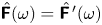
Force-statistic estimation (iii) was performed using the CSD of an auxiliary set of sensors, referred to as  $y'$, that consisted of streamwise and wall-normal velocity perturbations at
 $y^{+}=5,10,15,20,35$ and
 $40$. The force CSD was estimated as
 \begin{equation} \skew4\hat{\boldsymbol{\mathsf{F}}} = \skew4\hat{\boldsymbol{\mathsf{T}}}_{\boldsymbol{f}}^{\ \prime} \skew4\hat{\boldsymbol{\mathsf{Y}}}^{\ \prime} \skew4\hat{\boldsymbol{\mathsf{T}}}_{\boldsymbol{f}}^{\ \prime}, \end{equation}
where  $\skew4\hat{\boldsymbol{\mathsf{Y}}}^{\,\prime}$ is the CSD of the auxiliary sensor set:
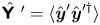 $\skew4\hat {\boldsymbol{\mathsf{Y}}}^{\ \prime} =\langle \hat {\boldsymbol {y}}' \hat {\boldsymbol {y}}'^{\dagger } \rangle$, and
 $\skew3\hat {\boldsymbol{\mathsf{T}}}_{\boldsymbol {f}}^{\ \prime}$ is the equivalent of (2.18) constructed for the auxiliary set of sensors
 $\boldsymbol {y}'$. This is similar to the procedure in Towne etal. (Reference Towne, Lozano-Durán and Yang2020), with the difference that here the estimated force CSD is used to improve estimation using a different set of measurements. Note that
 $\skew4\hat {\boldsymbol{\mathsf{Y}}}^{\,\prime}$ can be constructed in experiments using only two sensors. The auxiliary sensors are not used in the flow estimation described next. The choice of sensors was motivated by Nogueira etal. (Reference Nogueira, Morra, Martini, Cavalieri and Henningson2020), where correlations between wall-normal velocities and streamwise forces is shown to be important for the flow dynamics. Force CSDs for
 $\lambda _t^{+}=100$, where
 $\lambda _t^{+} = 2\pi /\omega ^{+}$ denotes the period in inner units, obtained directly from the DNS and estimated using the auxiliary sensors are shown in figure 27. The estimated colour has considerable differences when compared to the true colour. Nevertheless, as will be shown next, it contains the necessary information for an accurate state estimation.
Force CSDs ( $\skew3\hat {\boldsymbol{\mathsf{F}}}\,$) for
 $\lambda _t^{+} =100$ obtained directly form DNS data (Morra Reference Morra2020) (
 $a$) and estimated using the extra sensor set (
 $b$). Colour scale is saturated for the
 $\skew3\hat {\boldsymbol{\mathsf{F}}}_{f_x,f_x}$ component, which is an order of magnitude greater than the others as to make cross-correlations clearer.

A comparison of power spectral densities (PSD) obtained from the DNS and estimation at  $y^{+}=12$, where the PSD of the streamwise velocity component peaks, is presented in figure 28. The PSD for
 $\lambda _t^{+} = 100$ at different wall-normal positions is show in figure 29, and a time-series comparison is provided in figure 30. The largest velocity fluctuations are in the streamwise direction, and it is therefore the component for which estimation performance is best.
Turbulent-channel power-spectral densities for  $\lambda _{t}^{+} = 100$ of
 $u$,
 $v$ and
 $w$ from DNS and estimation using a different assumption of force statistics.

Turbulent-channel power-spectral densities of  $u$ at
 $y^{+} =12$ obtained from the DNS and estimation using a different assumption of force statistics.

Turbulent-channel streamwise velocity perturbation time series obtained from the DNS and estimation using a different assumption of force statistics. Estimation at  $y^{+}=12$.

The assumption of white-noise force in time and space does not provide a satisfactory flow estimation, as previously observed by Chevalier etal. (Reference Chevalier, Hœpffner, Bewley and Henningson2006). Studying the structure of the nonlinear force terms, Nogueira etal. (Reference Nogueira, Morra, Martini, Cavalieri and Henningson2020) showed that streaks generated by the lift-up mechanism have their amplitudes reduced by streamwise forces. This effect is not present if forces are assumed to be spatiotemporally white, leading to the overshoot observed in figure 28.
Chevalier etal. (Reference Chevalier, Hœpffner, Bewley and Henningson2006) explored spatial colouring of the forces, which were nonetheless simplified as white noise in time, probably due to the complexity of including full colour information in a Kalman-filter estimation. To the best of the authors’ knowledge, no previous study has included full force colour. With the resolvent-based estimation procedure we propose, estimation of relevant force components and their use for response estimation is straightforward.
The use of spatiotemporal forcing colour provides significant improvements in estimation performance. Low-rank forcing models can easily be obtained from experimental set-ups from sensor CSDs and the resolvent operator, and can thus be a useful tool to estimate full flow states in experimental set-ups, where one is typically limited to low-rank observations of the system.
5. Conclusions
We have presented an optimal method for the estimation of unsteady flow dynamics from sparse measurements. The approach is a generalization of the work of Towne etal. (Reference Towne, Lozano-Durán and Yang2020) and includes both force colour and sensor noise. Due to the explicit appearance of the resolvent operator, we refer to the method as resolvent-based estimation.
The method is suitable for application in transitional and turbulent flows. In the latter case the inhomogeneous linearised Navier–Stokes system is considered, nonlinear interactions being treated by means of an external forcing (McKeon & Sharma Reference McKeon and Sharma2010). Comparison with Kalman-filter estimation shows the resolvent-based approach to provide equal or better performance. A matrix-free procedure, involving the integration of one direct and one adjoint equation for each sensor, is elaborated that makes the method suitable for application in complex flows. Higher accuracy, lower computational cost and a simpler implementation renders the method attractive for the post-processing of experimental data.
When the resolvent-based estimator is truncated to its causal component it is shown to be equivalent to Kalman-filter estimation in certain scenarios. The approach may thus provide a viable means by which to perform real-time estimation and control of large systems without requiring the construction of reduced-order models.
In addition to clear computational benefits, the method provides a framework for interpretation of the mechanics of estimation. The foundation of this is resolvent analysis, which recent studies have shown to be a promising tool for the study and modelling of turbulent flows (McKeon & Sharma Reference McKeon and Sharma2010; Abreu etal. Reference Abreu, Cavalieri and Wolf2017; Beneddine etal. Reference Beneddine, Yegavian, Sipp and Leclaire2017; Schmidt etal. Reference Schmidt, Towne, Rigas, Colonius and Brès2018; Yeh & Taira Reference Yeh and Taira2019; Nogueira etal. Reference Nogueira, Morra, Martini, Cavalieri and Henningson2020; Towne etal. Reference Towne, Lozano-Durán and Yang2020). Thanks to this framework, the resolvent-based estimation can be understood in terms of an observable forcing subspace associated with the sparse measurements. Estimation accuracy depends on the extent to which the key forcing activity is observable by the sensors. Furthermore, we have shown that with limited knowledge of underlying force correlations, or a model of these, information from unobservable regions of the force space can be leveraged for estimation thanks to their correlation with the observable subspace. We show, using a turbulent channel flow, how modelling of the force statistics is necessary for accurate estimation.
Acknowledgments
A.V.G.C. was supported by CNPq, grant 310523/2017-6. E.M. acknowledges financial support from CAPES, grant 88881.190271/2018-01.
Declaration of interests
The authors report no conflict of interest.
Appendix A. Expressions for sensor noises correlated with forces
Given the system
 \begin{gather} \dfrac{\textrm{d}\boldsymbol{u}}{\textrm{d}t}(t) = \boldsymbol{\mathsf{A}} \boldsymbol{u}(t) + \boldsymbol{\mathsf{B}} \boldsymbol{f}(t), \end{gather}
 \begin{gather} \boldsymbol{y}(t) = \boldsymbol{\mathsf{C}} \boldsymbol{u}(t) + \boldsymbol{n}(t), \end{gather}
with
 \begin{equation} \langle \boldsymbol{f}(t) \boldsymbol{f}(t')^{\dagger}\rangle = \boldsymbol{\mathsf{F}}(t-t'), \quad \langle \boldsymbol{n}(t) \boldsymbol{n}(t')^{\dagger} \rangle = \boldsymbol{\mathsf{N}}(t-t'),\quad \langle \boldsymbol{n}(t) \boldsymbol{f}(t')^{\dagger} \rangle =\boldsymbol{\mathsf{M}} (t-t'). \end{equation}
Optimal force and state estimations, following an analogous derivation as presented in § 2, are stationary points of
 \begin{align} \langle\hat{\boldsymbol{e}}_u \hat{\boldsymbol{e}}_u^{\dagger}\rangle &= \langle \boldsymbol{\mathsf{R}} \boldsymbol{\mathsf{B}} \left(\skew2\hat{\boldsymbol{f}} - \skew4\hat{\boldsymbol{\mathsf{T}}}_{\boldsymbol{f}} \left(\boldsymbol{\mathsf{R}}_{\boldsymbol{y}}\skew2\hat{\boldsymbol{f}}+\hat{\boldsymbol{n}} \right)\right) \left(\skew2\hat{\boldsymbol{f}} - \skew4\hat{\boldsymbol{\mathsf{T}}}_{\boldsymbol{f}} \left(\boldsymbol{\mathsf{R}}_{\boldsymbol{y}} \skew2\hat{\boldsymbol{f}}+\hat{\boldsymbol{n}} \right) \right)^{\dagger} \boldsymbol{\mathsf{B}}^{\dagger} \boldsymbol{\mathsf{R}} ^{\dagger} \rangle \end{align}
 \begin{align} &= \boldsymbol{\mathsf{R}} \boldsymbol{\mathsf{B}} \Theta \boldsymbol{\mathsf{B}}^{\dagger} \boldsymbol{\mathsf{R}} ^{\dagger}, \end{align}
where
 \begin{align} \Theta & = \left(\boldsymbol{\mathsf{I}} -\skew4\hat{\boldsymbol{\mathsf{T}}}_{\boldsymbol{f}} \boldsymbol{\mathsf{R}}_{\boldsymbol{y}} \right) \skew4\hat{\boldsymbol{\mathsf{F}}} \left( \boldsymbol{\mathsf{I}} -\skew4\hat{\boldsymbol{\mathsf{T}}}_{\boldsymbol{f}} \boldsymbol{\mathsf{R}}_{\boldsymbol{y}} \right)^{\dagger} + \skew4\hat{\boldsymbol{\mathsf{T}}}_{\boldsymbol{f}} \skew2\hat{\boldsymbol{\mathsf{N}}} \skew4\hat{\boldsymbol{\mathsf{T}}}_{\boldsymbol{f}}^{\,\dagger} -\left( \boldsymbol{\mathsf{I}}-\skew4\hat{\boldsymbol{\mathsf{T}}}_{\boldsymbol{f}} \boldsymbol{\mathsf{R}}_{\boldsymbol{y}} \right) \boldsymbol{\mathsf{M}}^{\dagger}\skew4\hat{\boldsymbol{\mathsf{T}}}_{\boldsymbol{f}}^{\,\dagger} \nonumber\\ & \quad -\boldsymbol{\mathsf{M}}\skew4\hat{\boldsymbol{\mathsf{T}}}_{\boldsymbol{f}} \left( \boldsymbol{\mathsf{I}}-\skew4\hat{\boldsymbol{\mathsf{T}}}_{\boldsymbol{f}} \boldsymbol{\mathsf{R}}_{\boldsymbol{y}} \right)^{\dagger} \end{align}
for state estimation, and of
 \begin{equation} \left\langle\hat{\boldsymbol{e}}_f \hat{\boldsymbol{e}}_f^{\dagger}\right\rangle = \left\langle \left(\skew2\hat{\boldsymbol{f}} - \skew4\hat{\boldsymbol{\mathsf{T}}}_{\boldsymbol{f}} \left(\boldsymbol{\mathsf{R}}_{\boldsymbol{y}}\skew2\hat{\boldsymbol{f}}+\hat{\boldsymbol{n}} \right)\right) \left(\skew2\hat{\boldsymbol{f}} - \skew4\hat{\boldsymbol{\mathsf{T}}}_{\boldsymbol{f}} \left(\boldsymbol{\mathsf{R}}_{\boldsymbol{y}} \skew2\hat{\boldsymbol{f}}+\hat{\boldsymbol{n}} \right) \right)^{\dagger} \right\rangle = \Theta \end{equation}
for force estimation. Both stationary points are given by
 \begin{equation} \skew4\hat{\boldsymbol{\mathsf{T}}}_{\boldsymbol{f}} = \left(\skew4\hat{\boldsymbol{\mathsf{F}}} \boldsymbol{\mathsf{R}}_{\boldsymbol{y}}^{\dagger} +\boldsymbol{\mathsf{M}}^{\dagger}\right) \left( \boldsymbol{\mathsf{R}}_{\boldsymbol{y}} \skew4\hat{\boldsymbol{\mathsf{F}}} \boldsymbol{\mathsf{R}}_{\boldsymbol{y}} ^{\,\dagger} + \skew2\hat{\boldsymbol{\mathsf{N}}} + \boldsymbol{\mathsf{R}}_{\boldsymbol{y}} \boldsymbol{\mathsf{M}}^{\dagger} + \boldsymbol{\mathsf{M}} \boldsymbol{\mathsf{R}}_{\boldsymbol{y}} ^{\,\dagger} \right)^{-1}. \end{equation}
Appendix B. Memory efficient estimation of flow snapshots
The estimation expression in (2.39) reads as
 \begin{equation} \hat{\tilde{\boldsymbol{u}}} = \boldsymbol{\mathsf{R}} \boldsymbol{\mathsf{R}}_{\boldsymbol{y}}^{\dagger} (\boldsymbol{\mathsf{R}}_{\boldsymbol{y}} \boldsymbol{\mathsf{R}}_{\boldsymbol{y}}^{\dagger} + \epsilon \boldsymbol{\mathsf{I}})^{-1} \hat{\boldsymbol{y}}. \end{equation}
From § 2.4, the terms  $\boldsymbol{\mathsf{R}}_{\boldsymbol {y}} \boldsymbol{\mathsf{R}}_{\boldsymbol {y}}^{\dagger }$ and
 $\boldsymbol{\mathsf{R}} \boldsymbol{\mathsf{R}}_{\boldsymbol {y}}^{\dagger }$ can be obtained from integration of the direct and adjoint equations as
 \begin{equation} \boldsymbol{\mathsf{R}} \boldsymbol{\mathsf{R}}_{\boldsymbol{y}}^{\dagger} = \hat{\boldsymbol{q}}\quad \text{and} \quad \boldsymbol{\mathsf{R}}_{\boldsymbol{y}} \boldsymbol{\mathsf{R}}_{\boldsymbol{y}}^{\dagger} = \boldsymbol{\mathsf{C}} \hat{\boldsymbol{q}}, \end{equation}
where  $\hat {\boldsymbol {q}}$ contains the Fourier transform of the direct systems response. In order to estimate one snapshot of the flow, the large convolutions can be avoided using the following strategy: constructing
 $\skew3\hat {\boldsymbol{\mathsf{G}}} = (\boldsymbol{\mathsf{R}}_{\boldsymbol {y}} \boldsymbol{\mathsf{R}}_{\boldsymbol {y}}^{\dagger } + \epsilon \boldsymbol{\mathsf{I}})^{-1} \hat { \boldsymbol {z}}$, which can be calculated using only sensor readings from the direct run and from the flow to be estimated. Estimations can be obtained as
 \begin{equation} \hat{\tilde{\boldsymbol{u}}}(\omega) = \hat{\boldsymbol{q}}(\omega) \skew2\hat{\boldsymbol{\mathsf{G}}}(\omega), \end{equation}
which in the time domain is expressed as
 \begin{equation} \tilde{\boldsymbol{u}}(t) = \int_{-\infty}^{\infty} \boldsymbol{q}(\tau) \boldsymbol{\mathsf{G}}(t-\tau)\,\textrm{d}\tau, \end{equation}
which amounts to a single integral to construct one estimated flow snapshot. Thus, the only large data operation is the weighted sums of snapshots of the direct run, and only requires storing one snapshot in memory at a time.



