I. INTRODUCTION
Nanoindentation has been widely used to measure the Young's modulus of materials over the past decade due to its effectiveness in measuring mechanical properties. The theoretical analysis for the indentation problem with a spherical tip on semi-infinite medium was initially provided by Hertz over a century ago using elasticity theory.Reference Hertz1,Reference Hertz2 Advancement in experimental techniques using indentation gave rise to further studies on this problem. SneddonReference Sneddon3 obtained a relation between load, indentation depth, and Young's modulus for tips that could be described as revolution of a smooth function. KingReference King4 provided an expression for load–displacement curves when indentation was performed by flat ended punches. The expression could then be used to determine Young's modulus of the sample. Pharr et al.Reference Pharr, Oliver and Brotzen5 extended the analysis in Ref. Reference Sneddon3 by looking into the derivative of load–displacement curve and showed that the relation between surface stiffness, contact area, and Young's modulus was independent of the tip shape. Based on this generalized relation and the experimental work by Doerner and Nix,Reference Doerner and Nix6 Oliver and PharrReference Pharr, Oliver and Brotzen5 provided a technique to measure Young's modulus from nanoindentation data, which was later widely accepted as a standard testing procedure. Details of the procedure will be discussed in the following sections.
Over the past two decades, the Oliver–Pharr model has been applied to analyze nanoindentation data collected from various kinds of samples, including thin films or coatings on substrates which is of specific interest for this study. However, it was reportedReference Hay and Crawford7–Reference Wei, Zhang, Chen, Luo, Liu and Guo10 that the film modulus calculated using the Oliver–Pharr model could be impacted by the substrate particularly when the discrepancy in stiffness between the moduli of the thin film and substrate is significant and the depth of indentation is very large. Modifications to the original Oliver–Pharr model were delivered by many researchers to address these concerns, including Doerner and Nix,Reference Doerner and Nix6 Gao,Reference Gao, Chiu and Lee11 Mencik et al.,Reference Mencik, Munz, Quandt, Weppelmann and Swain12 Saha and Nix,Reference Saha and Nix8 Li and Vlassak,Reference Li and Vlassak13 Wei et al.,Reference Wei, Zhang, Chen, Luo, Liu and Guo10 Zhou and Prorok,Reference Zhou and Prorok14 and more recently, Hay and Crawford.Reference Hay and Crawford7 It should be noted that all these modifications were based on different assumptions and consequently validity of these models varied with conditions test and material parameters. Yet to the knowledge of the authors of this study, comparison between validity of these models has seldom been done. In particular, the case where an elastoplastic film was much more compliant than the substrate has not been rigorously examined. In the case of nanoindentation tests on nanoscale films of polymers on inorganic substrates, maximum displacements readily approach 40% of the film thickness, even under very low loadings. Thus, a detailed understanding of the models' performance in these conditions is needed.Reference Watcharotone, Wood, Friedrich, Chen, Qiao, Putz and Brinson9,Reference Miyake, Satomi and Sasaki15
This study provides a critical and quantitative comparison between some of the widely used models with the help of finite element (FE) simulations of nanoindentation of a compliant film bonded to stiff substrate. In the following sections of the study, a brief description of several widely used nanoindentation models will be provided. A general form of these models is proposed such that the difference between these models is characterized by comparison of weighting factors. A direct method of removing substrate effect demonstrated in Ref. Reference Watcharotone, Wood, Friedrich, Chen, Qiao, Putz and Brinson9 is also discussed. A description of the FE simulated nanoindentation test follows. Load–displacement data are collected from simulated nanoindentation tests and then processed with the selected models. By comparing the input film modulus to FE and output film modulus from the models, the validity of these approaches is checked and compared over a range of experimental parameters. The results from the FE analysis are discussed and the different models are evaluated and compared to each other for the compliant film/stiff substrate system. Finally, a demonstration using experimental data is presented.
Before proceeding, it should be noted that some different semi-analytical models have also been developed to exclude the substrate effect. In contrast to the models discussed thus far, which focused mostly on developing approximate mathematical methods to correct substrate effect based on the Oliver–Pharr method, some studies have been dedicated to understand the stress and strain fields generated in the film due to indentation. In the semi-analytical methods, a numerical solution is sought for the problem well defined by elasticity theory. For instance, ChenReference Chen16 and Chen and EngelReference Chen and Engel17 decomposed the stress field in purely elastic layered medium experiencing indentation as a combination of eigenfunctions with respect to thickness over contact radius. Yu et al.Reference Yu, Sanday and Rath18 developed another solution for the same problem with the help of a numerically solved Fredholm integral equation. Implementation of this method to elastoplastic film was provided by Zhao et al.Reference Zhao, Chen, Xiang, Vlassak, Lee, Ogasawara, Chiba and Gan19 Da Silva Botelho et al.Reference Da Silva Botelho, Progri, Inglebert and Robbe-Valloire20 further investigated into this problem by adopting Chen's previous work into Hertz's solution, with an additional assumption that strain was constant through the thickness of the film. Chen et al.Reference Chen, Zhou, Keer and Wang21 also developed another semi-analytical code to simulate the stress field of indentation based on the Chen's theory. The equivalent inclusion method was combined with continuous gradient methodReference Polonsky and Keer22 and used fast Fourier transform algorithmReference Liu, Wang and Liu23 to lower the computational cost. Although all these methods were of great value in understanding the indentation problem, they do not focus on direct analysis of the load–displacement data following the procedure used in the experiments and thus are not further considered in this study.
A. Oliver–Pharr model
Oliver and PharrReference Oliver and Pharr24–Reference Pharr, Strader and Oliver26 developed the most widely used nanoindentation model based on Sneddon's theoretical analysis in 1965 (Ref. Reference Sneddon3) and experimental work completed by Doerner and Nix.Reference Doerner and Nix6 This model can be credited with two significant advantages. First, a power function was used to describe the load–displacement at unloading stage, instead of the linear function as in Ref. Reference Doerner and Nix6. This led to improved accuracy when fitting the experimental data. Furthermore, the analysis in Ref. Reference Sneddon3 was extended. Using the initial slope of the unloading curve, the reduced modulus could be obtained from a simple expression that was independent of indenter tip geometry as long as the tip could be described as a revolution of a smooth function. If the tip geometry was not axisymmetric, for example, a pyramid tip or Berkovich tip, this general expression was also applicable after a correction parameter was implemented. These two advancements made it possible for material modulus to be obtained with considerable accuracy directly from load–displacement curves without any measurement of the indent on the sample. Nanoindentation tests were consequently simplified by this procedure and thus the Oliver–Pharr method was widely taken as a standard approach for measurement of modulus from indentation. Below, the derivation in Ref. Reference Pharr, Oliver and Brotzen5 is briefly revisited to facilitate the comparison to other models.
Assuming that the unloading process was purely elastic, SneddonReference Sneddon3 gave the expression for tip displacement, h, and load, P within the contact region indented by an axisymmetric tip. Pharr et al.Reference Pharr, Oliver and Brotzen5 continued this work and defined the surface stiffness, S, as:
 $$S = \beta {{{\rm{d}}P} \over {{\rm{d}}h}} = {{4\mu r} \over {1 - \nu }} = {2 \over {\sqrt \pi }}\sqrt {{A_{\rm{c}}}} {{{E_{\rm{r}}}} \over {1 - {\nu ^2}}}\quad ,$$
where μ and ν are the shear modulus and the Poisson's ratio of the sample, respectively. A c is the projected contact area, r is the contact radius, and E r is the reduced modulus of the sample. Note that the expression of S is independent of tip geometry as long as the indenter is axisymmetric. β is a correction factor applied to Sneddon's original analysis, which is discussed in detail in Ref. Reference Hay, Bolshakov and Pharr27. Hereafter, in the model comparison work, we take β = 1.06 for the conical tip based on the results in Ref. Reference Hay, Bolshakov and Pharr27.
It was further demonstrated that the contact area could be determined by the contact depth which was calculated using the following equation:
 $${h_{\rm{c}}} = {h_{{\rm{max}}}} - \varepsilon {{{P_{{\rm{max}}}}} \over S}\quad ,$$
where h c is the contact depth, h max is the maximum penetration depth of the tip, ε is a coefficient related to shape of the tip, and P max is the penetrating force at h = h max. The film modulus can be obtained from E r, which is obtained by combining Eqs. (1) and (2), using the following expression:
 $${1 \over {{E_{\rm{r}}}}} = {{1 - \nu _{\rm{f}}^2} \over {{E_{\rm{f}}}}} + {{1 - \nu _{\rm{i}}^2} \over {{E_{\rm{i}}}}}\quad ,$$
where E f is the Young's modulus of the sample (in our case, film) (The subscript f is used in E f as the sample Young's modulus value for consistency since we are ultimately concerned with the film samples in this study. However, the Oliver–Pharr model as shown in Eq. (3) is generally applicable to any sample tested.), E i is the Young's modulus of indenter tip, νf is the sample Poisson's ratio, νi is the Poisson's ratio of indenter tip, and β is the correction factor for non-axisymmetric tips. The Oliver–Pharr model focused on load and displacement, which were readily accessible to the experiment. Since the authors have specific interest in polymeric films coated on silica substrates, the modulus of the indenter is much larger than that of the sample, effectively removing the second term on the right hand side of Eq. (3).
Further studyReference Pharr and Oliver28,Reference Chen, Chen and Ou29 showed that applying the Oliver–Pharr model to thin films on substrates resulted in overestimation of the film modulus when indentation depth was higher than 10% of the film thickness, which motivated refinements to the original method. Bolshakov and PharrReference Bolshakov and Pharr30 investigated the impact of pile-up and sink-in problem to reach a more accurate estimate for contact radius. Stone et al.Reference Stone, Yoder and Sproul31 and Saha and NixReference Saha and Nix8 suggested using P/S 2 to characterize the property of the material since it was independent of the contact area, especially in a case where film and substrate had similar moduli. Yet it should be noted that, the models reviewed in the following sections all use the Oliver–Pharr method to provide essential input.
B. Saha–Nix model
In their early model predating the Oliver–Pharr model, Doerner and NixReference Doerner and Nix6 pointed out that the elastic modulus could be better predicted from a series of tests with different indentation depths based on the Hertz's indentation theory. However, as the indentation depth approached film thickness, the reduced modulus would be influenced by the substrate modulus. To account for the “substrate effect”, Doerner and Nix proposed an empirical equation characterizing the relation between the reduced modulus and the indentation depth which could be approximately expressed using the following form:
 $${1 \over {{E_{\rm{r}}}}} = {{1 - \nu _{\rm{f}}^{\rm{2}}} \over {{E_{\rm{f}}}}}\left( {1 - {e^{{{ - \alpha t} \mathord{\left/ {\vphantom {{ - \alpha t} {{h_{\rm{c}}}}}} \right. \kern-\nulldelimiterspace} {{h_{\rm{c}}}}}}}} \right) + {{1 - \nu _{\rm{s}}^2} \over {{E_{\rm{s}}}}}{e^{{{ - \alpha t} \mathord{\left/ {\vphantom {{ - \alpha t} {{h_{\rm{c}}}}}} \right. \kern-\nulldelimiterspace} {{h_{\rm{c}}}}}}} + {{1 - \nu _{\rm{i}}^2} \over {{E_{\rm{i}}}}}\quad ,$$
where t is the film thickness and α = 0.25 is an empirical parameter obtained through fitting a series of indentation results. The subscript “s” refers to the substrate, whereas the superscripts “f” and “i” refer to the film and indenter tip as mentioned above. KingReference King4 modified this model for flat punches and found that α was not a constant but a function with respect to ratio between the shape of indenter tip and the film thickness. Following the King's notation, the equation reads as follows:
 $${1 \over {{E_{\rm{r}}}}} = {{1 - \nu _{\rm{f}}^2} \over {{E_{\rm{f}}}}}\left( {1 - {e^{{{ - \alpha t} \mathord{\left/ {\vphantom {{ - \alpha t} a}} \right. \kern-\nulldelimiterspace} a}}}} \right) + {{1 - \nu _{\rm{s}}^2} \over {{E_{\rm{s}}}}}{e^{{{ - \alpha t} \mathord{\left/ {\vphantom {{ - \alpha t} a}} \right. \kern-\nulldelimiterspace} a}}} + {{1 - \nu _{\rm{i}}^2} \over {{E_{\rm{i}}}}}\quad ,$$
where a is the square root of contact area. Numerical solution of α was calculated for different types of flat punch tip in Ref. Reference King4. To extend the King's analysis to nonflattened tips such as Berkovich tip, Saha and NixReference Saha and Nix8 assumed that indentation with flat punch on a film with thickness t was equivalent to indentation with Berkovich tip on the same film but with effective thickness given by (t − h max). Based on this assumption, Saha and Nix utilized α for a triangular flat punch given in Ref. Reference King4 to estimate the weighting function for a Berkovich tip. Hence Eq. (6) was obtained:
 $${1 \over {{E_{\rm{r}}}}} = {{1 - \nu _{\rm{f}}^{\rm{2}}} \over {{E_{\rm{f}}}}}\left( {1 - {e^{{{ - \alpha \left( {t - {h_{{\rm{max}}}}} \right)} \mathord{\left/ {\vphantom {{ - \alpha \left( {t - {h_{{\rm{max}}}}} \right)} a}} \right. \kern-\nulldelimiterspace} a}}}} \right) + {{1 - \nu _{\rm{s}}^{\rm{2}}} \over {{E_{\rm{s}}}}}{e^{{{ - \alpha \left( {t - {h_{{\rm{max}}}}} \right)} \mathord{\left/ {\vphantom {{ - \alpha \left( {t - {h_{{\rm{max}}}}} \right)} a}} \right. \kern-\nulldelimiterspace} a}}} + {{1 - \nu _{\rm{i}}^2} \over {{E_{\rm{i}}}}}\quad .$$
Compared with Eq. (3), Eq. (6) indicated that the measurement of Young's modulus using the Oliver–Pharr procedure would be influenced by the substrate when the indentation depth approaches the substrate. As the tip is usually far stiffer than film and substrate, the last term on the right hand side of Eq. (6) is neglected in the following discussion. Saha and NixReference Saha and Nix8 experimentally showed the substrate effect for nanoindentation of Al thin films of different thicknesses on different substrates using a Berkovich tip. Furthermore, they applied this model to remove the “substrate effect” from the experimental data.
C. Gao model
Based on the experimental results by Doerner and Nix,Reference Doerner and Nix6 Gao et al.Reference Gao, Chiu and Lee11 provided an analysis starting from the energy perturbation introduced by the flat-ended indenter tip. With the assumption of a constant strain field, Gao et al. applied Neuber's solution for stress and strain field of flat punch indenting on a homogeneous isotropic solid,Reference Neuber32 and consequently expressed the force–displacement relation as:
 $$P = {{4r{\mu _{\rm{s}}}h} \over {1 - {{{\nu _{\rm{f}}} - {\nu _{\rm{s}}}} \over {1 - {\nu _{\rm{s}}}}}{I_1}\left( {{t \mathord{\left/ {\vphantom {t r}} \right. \kern-\nulldelimiterspace} r}} \right) - {{{\mu _{\rm{f}}} - {\mu _{\rm{s}}}} \over {{\mu _{\rm{s}}}}}{I_0}\left( {{t \mathord{\left/ {\vphantom {t r}} \right. \kern-\nulldelimiterspace} r}} \right)}}\quad ,$$
where μf and μs are the shear moduli of film and substrate, respectively, whereas other variables are as previously defined. Gao et al. further demonstrated that this approximation had first order accuracy for conical and Berkovich tips.
The effective modulus of this film–substrate system is expressed as:
 $${{1 - {\nu _{\rm{r}}}} \over {{\mu _{\rm{r}}}}} = {{1 - {\nu _{\rm{s}}} - ({\nu _{\rm{f}}} - {\nu _{\rm{s}}}){I_{1\_{\rm{Gao}}}}\left( {{t \mathord{\left/ {\vphantom {t r}} \right. \kern-\nulldelimiterspace} r}} \right)} \over {{\mu _{\rm{s}}} + ({\mu _{\rm{f}}} - {\mu _{\rm{s}}}){I_{0\_{\rm{Gao}}}}\left( {{t \mathord{\left/ {\vphantom {t r}} \right. \kern-\nulldelimiterspace} r}} \right)}}\quad ,$$
where μr and νr are the effective shear modulus and the Poisson's ratio that corresponds to E r term in previous definition, respectively. The weighting integrals I 0_Gao and I 1_Gao are expressed as follows:
 $${I_{0\_{\rm{Gao}}}}\left( {t/r} \right) = {2 \over \pi }\;\arctan \;{t \over r} + {1 \over {2\pi \left( {1 - {\nu _{\rm{r}}}} \right)}}\left[ {\left( {1 - 2{\nu _{\rm{r}}}} \right){t \over r}\ln {{1 + {{\left( {t/r} \right)}^2}} \over {{{\left( {t/r} \right)}^2}}} - {{{{(t/r)}^2}} \over {1 + {{\left( {t/r} \right)}^2}}}} \right]\quad ,$$
 $${I_{1\_{\rm{Gao}}}}\left( {t/r} \right) = {2 \over \pi }\;\arctan \;{t \over r} + {1 \over \pi }\left( {{t \over r}} \right)\ln {{1 + {{\left( {t/r} \right)}^2}} \over {{{\left( {t/r} \right)}^2}}}\quad .$$
“Effective” Poisson's ratio of the system is expressed as:
 $${\nu _{\rm{r}}} = {\nu _{\rm{s}}} + \left( {{\nu _{\rm{f}}} - {\nu _{\rm{s}}}} \right){I_{1\_{\rm{Gao}}}}\quad .$$
Gao also suggested that this relation could be compared with the models presented in Refs. Reference Doerner and Nix6 and Reference King4, which was later implemented by Xu and Pharr.Reference Xu and Pharr33 The latter concluded that a linear combination of the King’s model as shown in Eq. (5) and the Gao model can be used to match analytical predictions to FE simulation. Note that even though the Gao's model is developed for a flat punch and thus will not be directly applicable to the axisymmetric indentation demonstrated further here, the form of the model and the weighting functions are useful in comparison and provide the basis for part of the next model.
D. Hay model
Gao's indentation model was further modified by SongReference Song34 to give a simpler form of solution by separating the impact of Poisson's ratio from Eq. (8). Hay and CrawfordReference Hay and Crawford7 modified the “Song–Pharr” modelReference Xu and Pharr33,Reference Song34 to include both hard film on soft substrate and soft film on hard substrate. The Hay model argued that the increasing film modulus from measurement was attributed to two factors, namely, (a) misprediction of contact area by the Oliver–Pharr model and (b) stronger impact of substrate stiffness to composite stiffness of film–substrate at higher indentation depth. Correspondingly the contact depth was corrected through measurement from FE results while a phenomenological spring model with a fitting parameter determined also from FE simulation results was utilized to account for the composite stiffness issue.Reference Hay and Crawford7
 $${1 \over {{\mu _{\rm{r}}}}} = {{1 - {I_{0\_{\rm{Hay}}}}} \over {{\mu _{\rm{s}}} + F{I_{0\_{\rm{Hay}}}}{\mu _{\rm{f}}}}} + {{{I_{0\_{\rm{Hay}}}}} \over {{\mu _{\rm{f}}}}}\quad ,$$
where F is a fitting parameter obtained from analyzing the simulation results. I 0_Hay is the weight function derived from the Gao's model with a film thickness correction suggested by Mencik,Reference Mencik, Munz, Quandt, Weppelmann and Swain12 which is expressed in the following equation,
 $${I_{0\_{\rm{Hay}}}} =\; {2 \over \pi }\;\arctan \;{{t - {h_{\rm{c}}}} \over r} + {1 \over {2\pi \left( {1 - \nu } \right)}}\left[ {\left( {1 - 2\nu } \right){{t - {h_{\rm{c}}}} \over r}\ln {{1 + {{\left[ {\left( {{{t - {h_{\rm{c}}}} \mathord{\left/ {\vphantom {{t - {h_{\rm{c}}}} r}} \right. \kern-\nulldelimiterspace} r}} \right)} \right]}^2}} \over {{{\left[ {\left( {{{t - {h_{\rm{c}}}} \mathord{\left/ {\vphantom {{t - {h_{\rm{c}}}} r}} \right. \kern-\nulldelimiterspace} r}} \right)} \right]}^2}}} - {{{{\left[ {\left( {{{t - {h_{\rm{c}}}} \mathord{\left/ {\vphantom {{t - {h_{\rm{c}}}} r}} \right. \kern-\nulldelimiterspace} r}} \right)} \right]}^2}} \over {1 + {{\left[ {\left( {{{t - {h_{\rm{c}}}} \mathord{\left/ {\vphantom {{t - {h_{\rm{c}}}} r}} \right. \kern-\nulldelimiterspace} r}} \right)} \right]}^2}}}} \right]\quad .$$
Note that in Ref. Reference Hay and Crawford7, in the simulation where the film was purely elastic material, the difference between the moduli obtained using contact areas calculated by the Oliver–Pharr model and measured in the FE simulation was only around 5%. Also note that in the case that the substrate is much stiffer than the film, which is of interest of this study, the second term at the right hand side of Eq. (12) is much more significant than the first term. Thus, the weight of the film modulus term in the Hay model is approximately I 0_Hay.
E. Comparison between weight functions
The models presented above were developed to correct substrate effect that results when applying the original Oliver–Pharr model to determine the modulus of thin film on a substrate. Although the details of the equations differed, a common feature of these models was that the film modulus term and the substrate modulus term are weighted using specific functions. Thus, it is of interest to present a direct comparison between weighting functions of the film modulus term in the different models, so that a better understanding of these models is achieved. This idea is similar to the comparison suggested by Gao et al. in Ref. Reference Gao, Chiu and Lee11. As shown below, the Saha–Nix, Gao, and Hay models are able to be transformed into the following general form:
 $${1 \over {{E_{\rm{r}}}}} = {{1 - \nu _{\rm{f}}^{\rm{2}}} \over {{E_{\rm{f}}}}}I + {{1 - \nu _{\rm{s}}^{\rm{2}}} \over {{E_{\rm{s}}}}}\left( {1 - I} \right)\quad ,$$
where I is the weight of film modulus in the expression of reduced modulus. Generally speaking, I ∼ 1 when maximum indentation depth is low, which indicates that tip is “sensing” the film only. When indentation depth is large, I ∼ 0, and the substrate plays a significant role. Transforming each model into the proposed general form, the expression of I in each model is obtained. Numerical comparison between these weight factors is performed for compliant films on stiff substrates. We also assume that the Poisson's ratio of both film and substrate is 0.25 and a conical tip with half angle as 70.3°, which is consistent with the parameters used in Ref. Reference Hay and Crawford7. Hence, the relation between the geometric parameters, i.e., a, h c, and r is:
 $$a = 4.95{h_{\rm{c}}},\;r = 2.79{h_{\rm{c}}}\quad .$$
The Gao model is developed for a flat-ended punch and thus not completely suitable for indentation with conical tip, however, it is still compared with other models here for completeness since the modified form of the derived parameters from the Gao model is used in the Hay model.Reference Hay and Crawford7 Hereafter, the expression of the Gao model [Eq. (8)] is transformed into the following equation to perform the comparison,
 $${1 \over {{E_{\rm{r}}}}} = {{1 - \nu _{\rm{f}}^2} \over {{E_{\rm{f}}}}}{I_{{\rm{Gao}}}} + {{1 - \nu _{\rm{s}}^2} \over {{E_{\rm{s}}}}}\left( {1 - {I_{{\rm{Gao}}}}} \right)\quad ,$$
where I Gao is the weight function of film modulus in the Gao model. To obtain I Gao, we first express the left hand side of Eq. (16), i.e., 1/E r in terms of μr and νr:
 $${1 \over {{E_{\rm{r}}}}} = {1 \over {2{\mu _{\rm{r}}}\left( {1 + {\nu _{\rm{r}}}} \right)}}\quad .$$
Combining Eqs. (8) and (11), one can express Eq. (17) as:
 $${1 \over {{E_{\rm{r}}}}} = {1 \over {2\left[ {{\mu _{\rm{s}}} + \left( {{\mu _{\rm{f}}} - {\mu _{\rm{s}}}} \right){I_{{\rm{0\_Gao}}}}} \right]\left[ {1 + {\nu _{\rm{s}}} + \left( {{\nu _{\rm{f}}} - {\nu _{\rm{s}}}} \right){I_{{\rm{1\_Gao}}}}} \right]}}\quad .$$
In the meantime, Eq. (16) can also be expressed as:
 $${1 \over {{E_{\rm{r}}}}} = \left( {{{1 - {\nu _{\rm{f}}}} \over {2{\mu _{\rm{f}}}}} - {{1 - {\nu _{\rm{s}}}} \over {2{\mu _{\rm{s}}}}}} \right){I_{{\rm{Gao}}}} + {{1 - {\nu _{\rm{s}}}} \over {2{\mu _{\rm{s}}}}}\quad .$$
Combining Eqs. (18) and (19), one can express I Gao as:
 $${ {I_{{\rm{Gao}}}} = {{{1 \over {2\left[ {{\mu _{\rm{s}}} + \left( {{\mu _{\rm{f}}} - {\mu _{\rm{s}}}} \right){I_{0\_{\rm{Gao}}}}} \right]\left[ {1 + {\nu _{\rm{s}}} + \left( {{\nu _{\rm{f}}} - {\nu _{\rm{s}}}} \right){I_{1\_{\rm{Gao}}}}} \right]}} - {{1 - {\nu _{\rm{s}}}} \over {2{\mu _{\rm{s}}}}}} \over {{{1 - {{\rm{\nu }}_{\rm{f}}}} \over {2{{\rm{\mu }}_{\rm{f}}}}} - {{1 - {{\rm{\nu }}_{\rm{s}}}} \over {2{{\rm{\mu }}_{\rm{s}}}}}}} \cr = {{{{{\mu _{\rm{f}}}} \over {{\mu _{\rm{s}}}}} \cdot \left[ {{1 \over {\left( {1 - {I_{0\_{\rm{Gao}}}}} \right) + {{{\mu _{\rm{f}}}} \over {{\mu _{\rm{s}}}}}{I_{0\_{\rm{Gao}}}}}} \cdot {1 \over {1 + {\nu _{\rm{s}}} + \left( {{\nu _{\rm{f}}} - {\nu _{\rm{s}}}} \right){I_{1\_{\rm{Gao}}}}}} - \left( {1 - {\nu _{\rm{s}}}} \right)} \right]} \over {\left( {1 - {\nu _{\rm{f}}}} \right) - \left( {1 - {\nu _{\rm{s}}}} \right){{{\mu _{\rm{f}}}} \over {{\mu _{\rm{s}}}}}}}\quad . \cr}$$
As mentioned above, both the film and the substrate are with the same Poisson's ratio which is also the effective Poisson's ratio of the system, i.e., νr = νf = νs. In this case, the ratio between shear moduli of the film and the substrate equals to that of Young's moduli, i.e., μf/μs = E f/E s. Hence Eq. (20) can be simplified as:
 $$ {I_{{\rm{Gao}}}} = {{{{{E_{\rm{f}}}} \over {{E_{\rm{s}}}}} \cdot \left[ {{1 \over {\left( {1 - {I_{0\_{\rm{Gao}}}}} \right) + {{{E_{\rm{f}}}} \over {{E_{\rm{s}}}}}{I_{0\_{\rm{Gao}}}}}} \cdot {1 \over {1 + {\nu _{\rm{r}}} + \left( {{\nu _{\rm{r}}} - {\nu _{\rm{r}}}} \right){I_{1\_{\rm{Gao}}}}}} - \left( {1 - {\nu _{\rm{r}}}} \right)} \right]} \over {\left( {1 - {\nu _{\rm{r}}}} \right) - \left( {1 - {\nu _{\rm{r}}}} \right){{{E_{\rm{f}}}} \over {{E_{\rm{s}}}}}}}= {1 \over {\left( {1 - {\nu _{\rm{r}}}} \right)}}{{{{{E_{\rm{f}}}} \over {{E_{\rm{s}}}}}} \over {\left( {1 - {{{E_{\rm{f}}}} \over {{E_{\rm{s}}}}}} \right)}}\left[ {{1 \over {\left( {1 - {I_{0\_{\rm{Gao}}}}} \right) + {{{E_{\rm{f}}}} \over {{E_{\rm{s}}}}}{I_{0\_{\rm{Gao}}}}}} \cdot {1 \over {1 + {\nu _{\rm{r}}}}} - \left( {1 - {\nu _{\rm{r}}}} \right)} \right] = {{{{{E_{\rm{f}}}} \over {{E_{\rm{s}}}}}} \over {\left( {1 - {{{E_{\rm{f}}}} \over {{E_{\rm{s}}}}}} \right)}}\left[ {{1 \over {\left( {1 - {I_{0\_{\rm{Gao}}}}} \right) + {{{E_{\rm{f}}}} \over {{E_{\rm{s}}}}}{I_{0\_{\rm{Gao}}}}}} \cdot {1 \over {1 - \nu _{\rm{r}}^{\rm{2}}}} - 1} \right]\quad . \cr}$$
Modification is needed when the Saha–Nix model is applied to a conical tip since it is originally developed for Berkovich tip. Two terms are adjusted here. First, the effective normalized indentation depth is changed from (t − h max)/a to (t − h c)/r which follows the dimensionless scaling factor used in Ref. Reference Hay and Crawford7, instead of (t − h max)/a in Ref. Reference Saha and Nix8. Moreover, α in Ref. Reference Saha and Nix8, which is originally obtained in Ref. Reference King4 to evaluate weight function of the film modulus term when a triangular flat punch is used as the tip, is replaced with α in Ref. Reference King4 for circular punch since a conical tip is assumed here and also in the FE simulation section. Equation (6) is hence transformed to:
 $${1 \over {{E_{\rm{r}}}}} = {{1 - \nu _{\rm{f}}^2} \over {{E_{\rm{f}}}}}\left( {1 - {e^{{{ - \alpha \left( {t - {h_{\rm{c}}}} \right)} \mathord{\left/ {\vphantom {{ - \alpha \left( {t - {h_{\rm{c}}}} \right)} r}} \right. \kern-\nulldelimiterspace} r}}}} \right) + {{1 - \nu _{\rm{s}}^2} \over {{E_{\rm{s}}}}}{e^{{{ - \alpha \left( {t - {h_{\rm{c}}}} \right)} \mathord{\left/ {\vphantom {{ - \alpha \left( {t - {h_{\rm{c}}}} \right)} r}} \right. \kern-\nulldelimiterspace} r}}}\quad .$$
In which weight of film modulus term in the Saha–Nix model is obtained for conical tip:
 $${I_{{\rm{SN}}}} = 1 - \exp \left( { - \alpha {{t - {h_{\rm{c}}}} \over r}} \right)\quad .$$
Assuming that the substrate is much stiffer than the film, we wish to find a generalized weight factor, I Hay, that allows us to express the Hay model in the form of Eq. (14):
 $${1 \over {{E_{\rm{r}}}}} = {{1 - \nu _{\rm{f}}^2} \over {{E_{\rm{f}}}}}{I_{{\rm{Hay}}}} + {{1 - \nu _{\rm{s}}^2} \over {{E_{\rm{s}}}}}\left( {1 - {I_{{\rm{Hay}}}}} \right)\quad .$$
With the prescribed assumption, Eq. (12) can be expressed in terms of Young's modulus and Poisson's ratio, as shown below:
 $${1 \over {{{{E_{\rm{r}}}} \over {2\left( {1 + {\nu _{\rm{r}}}} \right)}}}} = {{1 - {I_{0\_{\rm{Hay}}}}} \over {{{{E_{\rm{s}}}} \over {2\left( {1 + {\nu _{\rm{s}}}} \right)}} + F{I_{0\_{\rm{Hay}}}}{{{E_{\rm{f}}}} \over {2\left( {1 + {\nu _{\rm{f}}}} \right)}}}} + {{{I_{0\_{\rm{Hay}}}}} \over {{{{E_{\rm{f}}}} \over {2\left( {1 + {\nu _{\rm{f}}}} \right)}}}}\quad .$$
Equation (25) can also be simplified with the prescribed assumption that νr = νf = ν = 0.25s:
 $${1 \over {{E_{\rm{r}}}}} = {{1 - {I_{{\rm{0\_Hay}}}}} \over {{E_{\rm{s}}} + F{I_{{\rm{0\_Hay}}}}{E_{\rm{f}}}}} + {{{I_{{\rm{0\_Hay}}}}} \over {{E_{\rm{f}}}}}\quad .$$
Combining Eqs. (24) and (26) to eliminate the E r term, the weight function in the Hay model can be expressed as:
 $${ {I_{{\rm{Hay}}}} = {{{{{I_{0\_{\rm{Hay}}}}} \over {{E_{\rm{f}}}}} + {{1 - {I_{0\_{\rm{Hay}}}}} \over {{E_{\rm{s}}} + F{I_{0\_{\rm{Hay}}}}{E_{\rm{f}}}}} - {{1 - \nu _{\rm{r}}^{\rm{2}}} \over {{E_{\rm{s}}}}}} \over {{{1 - \nu _{\rm{r}}^{\rm{2}}} \over {{E_{\rm{f}}}}} - {{1 - \nu _{\rm{r}}^{\rm{2}}} \over {{E_{\rm{s}}}}}}} = {1 \over {1 - \nu _{\rm{r}}^{\rm{2}}}}{{{I_{0\_{\rm{Hay}}}} + {{{E_{\rm{f}}}\left( {1 - {I_{0\_{\rm{Hay}}}}} \right)} \over {{E_{\rm{s}}} + F{I_{0\_{\rm{Hay}}}}{E_{\rm{f}}}}} - {{{E_{\rm{f}}}} \over {{E_{\rm{s}}}}}\left( {1 - \nu _{\rm{r}}^{\rm{2}}} \right)} \over {\left( {1 - {{{E_{\rm{f}}}} \over {{E_{\rm{s}}}}}} \right)}}\quad . \cr}$$
Since E f < E s as assumed here and the constant F = 0.0626,Reference Hay and Crawford7 FI 0_HayE f « E s. Under this assumption, the Hay model converges to Song–Pharr modelReference Xu and Pharr33,Reference Song34 and Eq. (27) can be further simplified into the following form:
 $${ {I_{{\rm{Hay}}}} = {1 \over {1 - \nu _{\rm{r}}^{\rm{2}}}}{{{I_{0\_{\rm{Hay}}}} + {{{E_{\rm{f}}}} \over {{E_{\rm{s}}}}}\left( {1 - {I_{0\_{\rm{Hay}}}}} \right) - {{{E_{\rm{f}}}} \over {{E_{\rm{s}}}}}\left( {1 - \nu _{\rm{r}}^{\rm{2}}} \right)} \over {\left( {1 - {{{E_{\rm{f}}}} \over {{E_{\rm{s}}}}}} \right)}} & <$$><$$>= {1 \over {1 - \nu _{\rm{r}}^{\rm{2}}}}{{{I_{0\_{\rm{Hay}}}}\left( {1 - {{{E_{\rm{f}}}} \over {{E_{\rm{s}}}}}} \right) + {{{E_{\rm{f}}}} \over {{E_{\rm{s}}}}}\nu _{\rm{r}}^{\rm{2}}} \over {\left( {1 - {{{E_{\rm{f}}}} \over {{E_{\rm{s}}}}}} \right)}} & <$$><$$>= {1 \over {1 - \nu _{\rm{r}}^{\rm{2}}}}\left[ {{I_{0\_{\rm{Hay}}}} + {{{{{E_{\rm{f}}}} \over {{E_{\rm{s}}}}}\nu _{\rm{r}}^{\rm{2}}} \over {\left( {1 - {{{E_{\rm{f}}}} \over {{E_{\rm{s}}}}}} \right)}}} \right]\quad . &\cr}$$
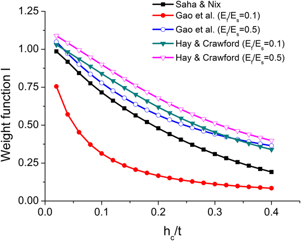
The weight functions of the film modulus term in the models discussed above are a function of contact depth, with E f, E s, Poisson's ratio, and film thickness given. With the expressions for weighting functions obtained for all the three models [Eqs. (20), (23), and (28)], a numerical comparison is shown in Fig. 1. Although the scaling factors are different in these models, they can all be converted to functions of h c/t with the help of Eq. (15). As I Gao and I Hay are explicitly dependent on the ratio of film modulus over substrate modulus, the ratio of E f/E s is set as 0.1 and 0.5 for illustration.
Comparison between weight of the film modulus term in different models contact depth normalized by film thickness.

The magnitude of the correction differs significantly across the modulus as can be seen in Fig. 1. At small indentation depths, the weighting function I in most of the models approaches 1, indicating that only film modulus is sensed, providing results similar to the Oliver–Pharr model in Eq. (3). When the indentation depth is large, however, the weighting functions decrease and thus the film moduli extracted from these models are lower than that from the Oliver–Pharr model. Thus, the overestimation of film modulus when indentation is performed on compliant films on a stiff substrate is improved by these models. To directly examine the validity of these models when applied to elastic–plastic materials, a FE simulation of nanoindentation is performed as described in “Methods” section. It should be noted that, however, the weight function of the Hay model exceeds the limit of unity at very shallow indentation depth. This fact, however, does not indicate the bound values of the Hay model were not carefully considered in the original work. The original weight function in the Hay model, i.e., I 0_Hay is strictly bounded to 0–1. Yet as we transform the Hay model into the form of Eq. (24), the weight function, I Hay, deviates from I 0_Hay due to the fact that we are calculating the Young's modulus in Eq. (24), rather than the shear modulus in the original Hay model.
F. Direct finite element method
An alternative approach to the numerical models reviewed in the previous sections is to use FE simulation to extract the substrate effect from experimental data directly.
Simulated nanoindentation tests via FE have been used to improve analysis on the data collected in experiments, as shown in Refs. Reference Hay and Crawford7 and Reference Cheng and Cheng35–Reference Chollacoop, Li and Gouldstone40. Cheng and Cheng,Reference Cheng and Cheng35 Knapp et al.,Reference Knapp, Follstaedt, Myers, Barbour and Friedmann36 and Zeng and ShenReference Zeng and Shen38 examined the error of h c determination in the indentation tests on materials with different mechanical properties using FE modeling. Xu and RowcliffeReference Xu and Rowcliffe39 checked the validity of the substrate effect predicted by the Doerner and Nix's modelReference Doerner and Nix6 when indentation simulation was performed on elastoplastic materials. Chollacoop et al.Reference Chollacoop, Li and Gouldstone40 predicted the error in modulus measurements of indentation tests on the film/substrate with similar modulus but different yield strength.
Another different approach is to use a series of FE models to explicitly calculate the substrate effect for different h c/t values for a soft film on a stiff substrate. The experimental results can then be directly corrected without applying empirical models and the real film modulus can be found. This strategy was implemented in Ref. Reference Watcharotone, Wood, Friedrich, Chen, Qiao, Putz and Brinson9 to correct the experimental results of indentation on compliant polymer films coated on stiff inorganic substrate. The existence of interphase polymer (altered polymer near the substrate) was assumed in the polymer films, which caused the measured elastic modulus of the film to deviate from that of the elastic modulus of the bulk film, E 0.
It was assumed in Ref. Reference Watcharotone, Wood, Friedrich, Chen, Qiao, Putz and Brinson9 that at each indentation depth:
 $$E_{{\rm{f}}\_{\rm{OP}}}^{{\rm{expt}}} = {E_{\rm{f}}} + E_{\rm{f}}^{{\rm{substrate}}\_{\rm{effect}}\_{\rm{expt}}}\quad ,$$
where OP and superscript expt indicates the
Oliver–Pharr approach, which was used on the experimental data.  $E_{\rm{f}}^{{\rm{substrate\_effect\_expt}}}$ is the deviation from true modulus value
caused by the substrate effect. Meanwhile, in the simulated nanoindentation
tests performed in FE, if the Oliver–Pharr approach was followed to
process the load–displacement data,
 $$E_{{\rm{f}}\_{\rm{OP}}}^{{\rm{FE}}} = E_{\rm{f}}^{{\rm{input}}} + E_{\rm{f}}^{{\rm{substrate}}\_{\rm{effect}}\_{\rm{FE}}}\quad ,$$
where superscript FE indicated that the data
were from FE simulation.  $E_{\rm{f}}^{{\rm{substrate}}\_{\rm{effect}}\_{\rm{FE}}}$ was then obtained from Eq. (30) after FE simulation. The
substrate effect from FE normalized by the input film modulus can be related to
that from experiment normalized by an estimated true film modulus,
E 0, which in Ref. Reference Watcharotone, Wood, Friedrich, Chen, Qiao, Putz and Brinson9 is chosen as the Young's modulus of the film sample
with largest thickness measured at low indentation depth, which is believed to
be free of substrate effect.
 $${{E_{\rm{f}}^{{\rm{substrate}}\_{\rm{effect}}\_{\rm{FE}}}} \over {E_{\rm{f}}^{{\rm{input}}}}} = {{E_{\rm{f}}^{{\rm{substrate}}\_{\rm{effect}}\_{\rm{expt}}}} \over {{E_0}}}\quad .$$
Thus, the true film modulus, i.e., E f could be expressed as:
 $${ {E_{\rm{f}}} = E_{{\rm{f}}\_{\rm{OP}}}^{{\rm{expt}}} - E_{\rm{f}}^{{\rm{substrate}}\_{\rm{effect}}\_{\rm{expt}}} <$$><$$>= E_{{\rm{f}}\_{\rm{OP}}}^{{\rm{expt}}} - {E_0}{{E_{\rm{f}}^{{\rm{substrate}}\_{\rm{effect}}\_{\rm{FE}}}} \over {E_{\rm{f}}^{{\rm{input}}}}} <$$><$$> = E_{{\rm{f}}\_{\rm{OP}}}^{{\rm{expt}}} - {E_0}{{E_{{\rm{f}}\_{\rm{OP}}}^{{\rm{FE}}} - E_{\rm{f}}^{{\rm{input}}}} \over {E_{\rm{f}}^{{\rm{input}}}}} <$$><$$> = E_{{\rm{f}}\_{\rm{OP}}}^{{\rm{expt}}} + {E_0} - {E_0}{{E_{{\rm{f}}\_{\rm{OP}}}^{{\rm{FE}}}} \over {E_{\rm{f}}^{{\rm{input}}}}}\quad . \cr}$$
II. METHODS
In the case of indentation performed for polymeric films with elastoplastic constitutive relation coated on stiff substrates, the discrepancy between the moduli of film and the substrate can be from one to several orders of magnitude. Yet these models have not been validated under these conditions. Furthermore, while surface stiffness of the material is often assumed to be independent of the plasticity properties, for compliant elastoplastic films it has been observedReference Oliver and Pharr25,Reference Cheng and Cheng35,Reference Zeng and Shen38,Reference Chollacoop, Li and Gouldstone40 that the shape of the unloading curve varies with the ratio between modulus and yield strength of the film. Based on these considerations, we hereby present a thorough comparison of some of the widely used models with the help of FE simulation to improve understanding of the models' performance as well as to evaluate the possible errors incurred by the assumptions of each model when applied to elastoplastic film/substrate systems.
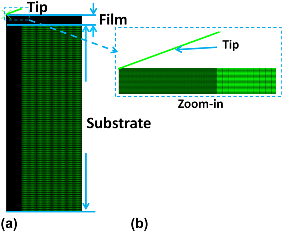
FE simulations of nanoindentation of thin films on a stiff substrate are carried out using the ABAQUS software package. Axisymmetric models are used as shown in Fig. 2. A conical tip with half angle of 70.3° is modeled. The film thickness is set to be 500 nm, whereas the thickness of the substrate is 10,000 nm. Both the film and substrate are 2000 nm in radius. Film and substrate are modeled as homogeneous materials and meshed with approximately 41,000 elements in total. The mesh is refined using triangular elements in regions where stress concentrations are expected. This refinement also ensures an accurate measurement of contact depth during post-processing. An elastic-perfectly plastic constitutive relation is assigned to film. When benchmarking with reported results in Ref. Reference Hay and Crawford7 we change the constitutive relation to linear elasticity to be consistent with FE models in Ref. Reference Hay and Crawford7. Although load is time-related in realistic experiments, we simplify the problem by using static steps of loading and unloading along with frictionless interaction along the tip–film interface and a perfect bonding at the film–substrate interface. The bottom boundary of the substrate is fixed along vertical direction and free to move along radial direction, while the lateral boundary of both film and substrate, shown on the right hand side of Fig. 2 left, is free to move. To avoid spurious penetration of the surface elements, a normal contact between tip and film is defined as “soft contact” in which an exponential function is used to describe the pressure-overclosure relation. The maximum indentation depth is set to 20–180 nm, which is 4–36% of the film thickness.
Mesh and geometry of FE model for model comparison. (a) Overview of meshed geometry. (b) Zoom-in of the tip contact region shown in (a).

The Oliver–Pharr method relies on contact depths predicted from a simple expression using indentation depth and information from the load–displacement curve, as shown in Eq. (2). This precludes the need for measurement of the contact depth from experiment that is not easily accessible during an indentation test. However, as plasticity is included in the FE model, pile-ups can lead to an error in determination of h cReference Cheng and Cheng35,Reference Tsui, Vlassak and Nix41 and consequently film modulus.Reference Hay and Crawford7 In the FE models, contact depth can be measured directly with the accuracy of the mesh size and compared to the prediction from the Oliver–Pharr approach. This procedure is demonstrated in the FE model in Ref. Reference Hay and Crawford7 and is followed here for measuring contact radius and depth. In this procedure, the boundary of the contact region is determined by locating the intersection of the lines defined by the last 2 nodes within contact and the first 2 nodes outside the contact.
The load–displacement data are obtained from the FE simulations. These data are then processed using each of the models exactly as experimental data would be, except that the contact area is obtained from both the load–displacement curve and the measured value in FE simulation for some of the models. Output film modulus with substrate effect removed by the models is compared to the known input modulus value. Calculations are repeated for various moduli input to the FE simulation over a range of E f/E s and indentation (h max/t) ratios. In all the tests, the E s is fixed to 100 GPa, with the yield stress of the substrate as 0.02E s. E f/E s is chosen as 5, 10, 20, 25, and 50%, where the lower end is representative of a typical glassy polymer film on the silica substrate. Two different E f/σy values (50 and 20) are considered in each case, where σy is the yield stress of the film.
III. RESULTS
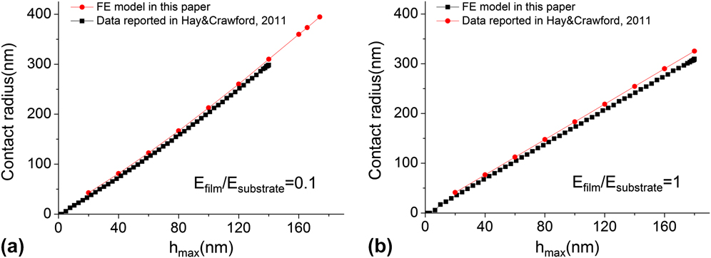
Hay and Crawford used a similar axisymmetric model to simulate nanoindentation test on film–substrate system.Reference Hay and Crawford7 We have benchmarked our FE model to the one described in Ref. Reference Hay and Crawford7 where a linear elastic constitutive law is assigned to film. After the simulated indentation test is performed, the contact radius is measured in FE and compared with the reported data in Ref. Reference Hay and Crawford7. Good agreement is found in contact radius as shown in Fig. 3, suggesting that our axisymmetric simulations are equivalent to the model used in Ref. Reference Hay and Crawford7.
Comparison between contact radii extracted from axisymmetric FE model and data obtained from the axisymmetric FE model reported in Ref. Reference Hay and Crawford7, when (a) E film/E substrate is equal to 0.1 and (b) E film/E substrate is equal to 1.

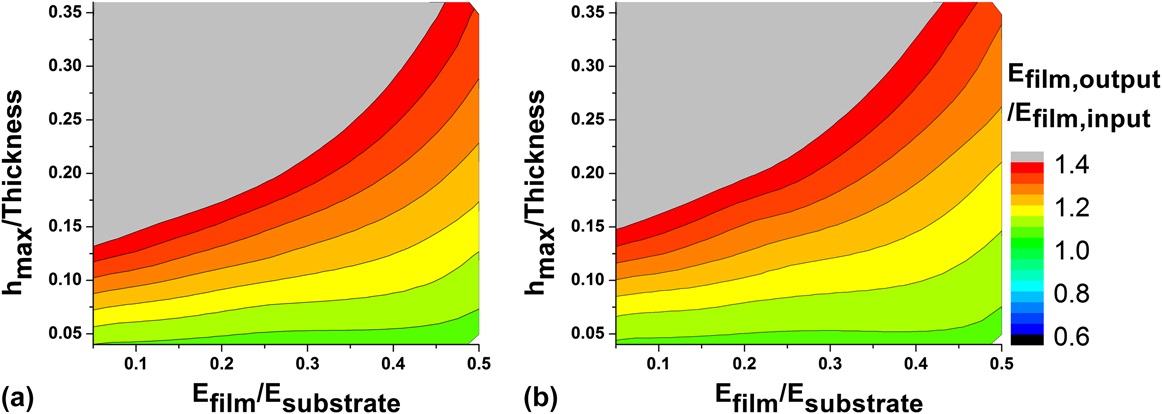
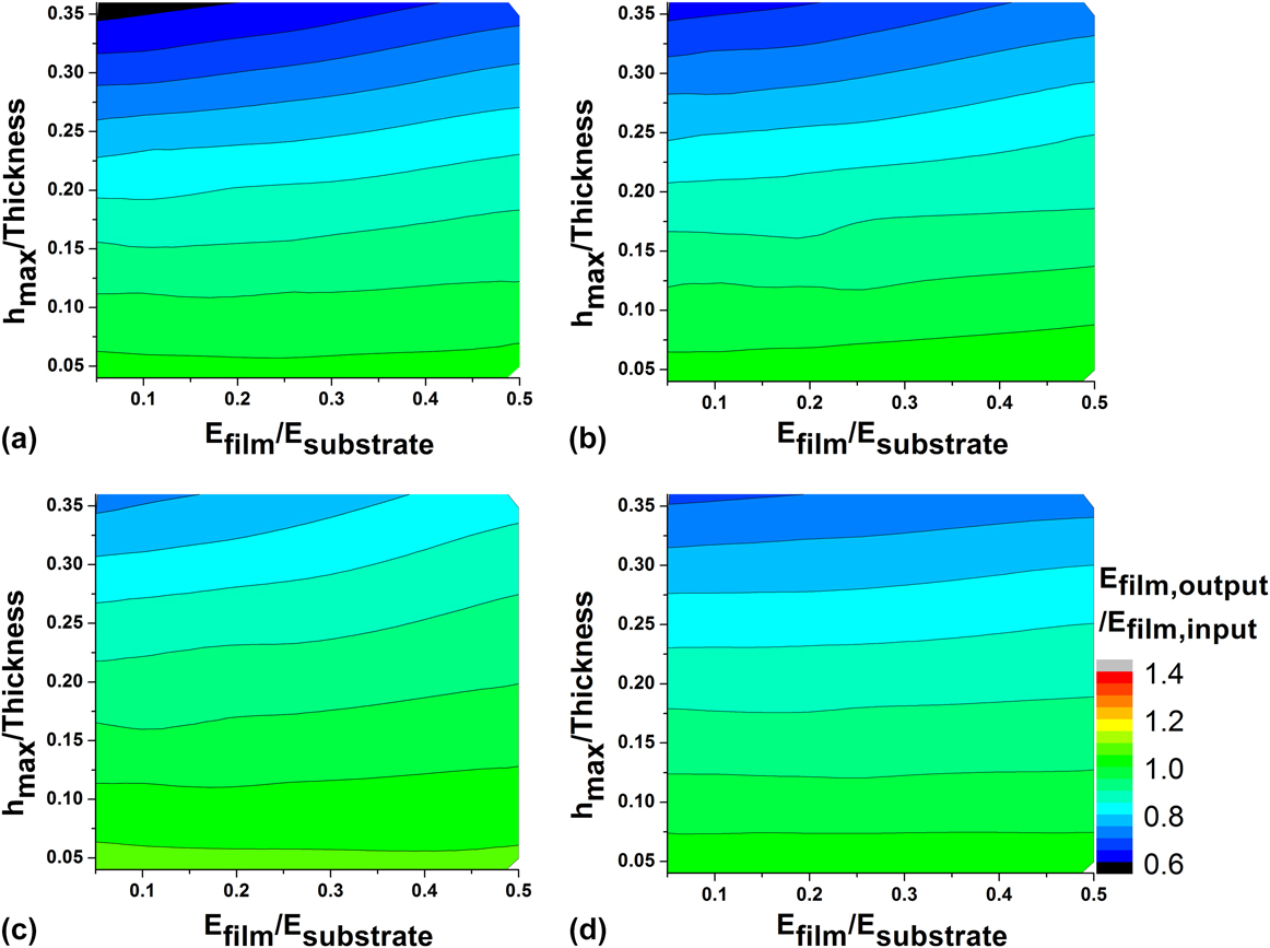
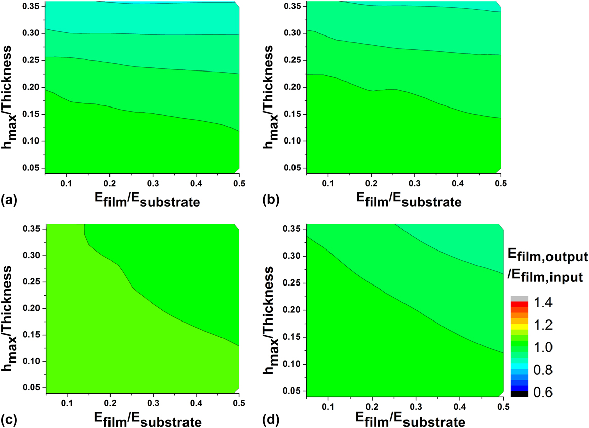
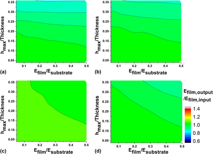
Three different models for various E f/E s are systematically applied over a range of h max/t for two different E f/σy ratios to probe the efficacy of these models in predicting the film modulus, as shown in Figs. 4–6. In each contour of Figs. 4–6, the green region indicates that predicted film moduli from the models are close to input film moduli (E film, output/E film, input = 1) at the given indenting ratio (max indentation depth/film thickness) and film/substrate modulus mismatch ratio (E f/E s). In these green regions, the substrate effect is considered to be fully removed. In contrast, in blue or red/gray regions, the predicted film moduli from the models are significantly smaller or larger than input film moduli. Thus, in the red, gray, or blue regions, the performance of the models is not acceptable under the given conditions.
E film, output/E film, input results are obtained using the Oliver–Pharr model with contact depth measured from FE simulation results. The data are reported for two values of E f/σy, (a) 50 and (b) 20.

E film, output/E film, input results for the Saha–Nix model, data in (a) and (b) are using corrected h c measured in the FE model as described in Ref. Reference Hay and Crawford7, whereas in (c) and (d) contact depth is extracted from fitting the load–displacement curve, as indicated in the Oliver–Pharr model in Eq. (2). Two values of E f/σy are reported, (a, c) 50 and (b, d) 20.

E film, output/E film, input results obtained from the Hay's model. Contact depth is measured in FE models as described in Ref. Reference Hay and Crawford7. Two values of E f/σy are reported, (a) 50 and (b) 20.

Figure 4 shows the film modulus calculated by the Oliver–Pharr method plotted as a control. Since the substrate effect is not considered in the original Oliver–Pharr model, the film moduli are dramatically over-predicted in nearly the entire testing range conducted here. Difference between output film moduli and input moduli is found to be relatively small only if E f is close to E s or indenting ratio is low (h max/t < 0.05).
Originally in the Saha–Nix model, h c is estimated only using the Oliver–Pharr method as shown in Eq. (2). We also considered using the h c correction demonstrated in the Hay model with the Saha–Nix model since h c is directly measured from simulation as mentioned above. Figure 5 shows the results of the Saha–Nix model with contact depth measured in FE model and predicted using Eq. (4) to evaluate its impact. Compared to the original Oliver–Pharr model (Fig. 4), the Saha–Nix model performs significantly better over a wider range of the parameters studied. However, it should be noted that in our case where the parameters in the Saha–Nix model are adjusted for the conical tip, the Saha–Nix model tends to underestimate the film modulus at high indentation ratio. After the contact depth correction using FE data [Figs. 5(a) and 5(b)], the underestimation is more significant.
Among all the models listed in this section, the Hay model with the contact depth from FE simulation gives the best overall performance, as shown in Fig. 6. At lower E f/E s ratios, it is more effective in matching the input modulus of the film in FE simulations. Although the calculated film modulus is slightly lower than the input modulus at very high indentation ratio, in general, it provides excellent results over a wider range of parameters studied.
Note that the Gao model is not compared directly in these examples since it is developed for a flat punch and therefore not directly applicable to the axisymmetric conical indentation demonstrated here. The direct FE approach, not shown, results in a perfect field of green for all indentation depths and film/substrate moduli since the FE simulation is the reference for all results.
IV. DISCUSSION
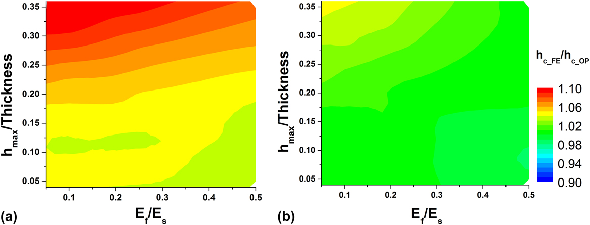
Although the unloading data from load–displacement were originally believed to involve only elastic properties,Reference Oliver and Pharr24 pile-up and sink-in are observed in indentations performed on elastoplastic materials, which accounts for the deviation of h c from the value predicted by Eq. (2).Reference Oliver and Pharr25,Reference Cheng and Cheng35,Reference Zeng and Shen38,Reference Chollacoop, Li and Gouldstone40 The FE simulation results in Figs. 4–6 show evidence to support that E f/σy can slightly impact the predicted moduli. This result is contrary to the commonly accepted conclusion that the reduced modulus determined from the load–displacement curve is completely independent of plasticity. It is observed in our FE simulation results that the load and the contact depth are both modestly affected by the change of yield stress for the model with the same film modulus. The comparison between the measured h c and the h c predicted using Eq. (2) is shown in Fig. 7 where around 5% difference in this ratio is observed between the two tested E f/σy. Though as reported in Ref. Reference Hay and Crawford7 Eq. (2) worked generally well for elastic films when E f < E s, our results show that larger deviations result for elastoplastic films. The h c correction increases in importance as the yield strength of the material decreases for a given film modulus.
Comparison between h c measured in FE model (E f/σy = 50) and h c predicted using Eq. (2). E f/σy = 50 in (a) and E f/σy = 20 in (b).

The Oliver–Pharr model was originally developed for bulk samples and does not explicitly account for the “substrate effect” that occurs when using nanoindentation to report the properties of thin films on substrates. Indeed, significant deviation of film modulus from known input is observed in cases where the film is much more compliant than substrate in Fig. 4. The current results also clearly demonstrate that high indenting ratios lead to dramatic overestimation of film modulus when the Oliver–Pharr approach is utilized to analyze the experimental data. However, this concern diminishes when the film modulus is comparable to the substrate modulus at low indenting ratios (E f/E s > 0.25 and h max/t < 0.05, green contours in Fig. 4).
The Saha–Nix model works generally well for compliant films, as the green region occupies the majority of the validity contours in Fig. 5. However, it should be noted that the film modulus from the Saha–Nix model deviates significantly from the input film modulus at high indenting ratios. As addressed in Ref. Reference Saha and Nix8, when E f/E s is small, the film modulus obtained from the Saha–Nix model is lower than expected. Additionally, it is found in our simulation that the underestimation of film modulus of the Saha–Nix model at high indentation ratio is also observed when the plasticity is included in the simulation. At low indentation ratio, the Saha–Nix model provides good estimation of film modulus as observed.
Furthermore, it is observed that when the “true contact depth” from FE is used to calculate weight functions in the Saha–Nix model [i.e., Figs. 5(a) and 5(b)], the underestimation of film modulus is generally more significant compared with the result from the same model but using the contact depth extracted from load–displacement curve with Eq. (2) [Figs. 5(c) and 5(d)]. Since parameters of the Saha–Nix model are calibrated based on the h c coming from Eq. (2), it does not perform as well when “true contact depth” is applied as shown in Fig. 5. In other words, the error in h c calculated from Eq. (2) partially balances the error in the analytical modulus calculations in Eq. (6) to provide “better” results. However, in other situations these errors might be additive. Contact depth from the Oliver–Pharr method is still commonly used in application since it can be easily calculated from experimental load–displacement curve without additional testing. Our results provide a note of caution regarding this application, especially in the case that the film material tends to yield at small strains.
The Hay model is also effective in predicting the film modulus within the parametric space as shown in Fig. 6, and performs better for compliant films on stiff substrates. With h c measured from simulation, it is shown in Ref. Reference Hay and Crawford7 that an almost perfect match is found between input and output moduli of FE modeling. While our results confirm the excellent performance of the Hay model when applied to elastoplastic films and using h c both from load–displacement data using Eq. (2) and direct measurement in the FE model, it also indicates that the Hay model is more accurate when the yield stress of the film is higher as a larger green region is observed in Figs. 6(b) and 6(d) compared to Figs. 6(a) and 6(c). Since the Hay model is tuned and examined for purely elastic films, this is actually expected. Application of the Hay model might also need caution if film yields at extremely small strain, but examining this case is beyond the scope of this study.
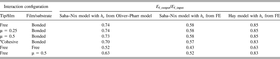
To examine the influence of the boundary conditions in both experimental and FE simulations, additional simulations are carried out on film/substrate systems with different contact properties, as shown in Table I. In these examples, E f/E s is maintained at 0.1 with E f/σy = 50 and the indenting ratio is held at 0.36, representative of a thin polymer film on a stiff substrate. The following cases are considered: (a) friction coefficient between tip and film surface (μ) of 0 (free), 0.25 or 0.5, (b) film and substrate interface varies from perfect bonding to friction coefficient of 0 (friction-free) or 0.5, and (c) cohesive interaction between tip and film, i.e., slight adhesion is assigned to the interface between tip and film, in which the additional traction on elements along the film surface is characterized by a linear function of separation between tip and film surfaces. The first (bolded) row in the table shows the results under the same condition considered for all simulations earlier in this study. The assumption of the frictionless interaction between the tip and the film is also applied in the models chosen for comparison. It is noted that by adding the friction or cohesive interaction between the film and the tip into the FE simulation, the calculated film modulus only slightly differs from the value in the frictionless model, which validates such assumption. One observes from the last two rows that altering interaction between film and substrate can result in significant changes in the measured modulus. It indicates that if a delamination between the film and the substrate takes place in the experiments, the film modulus will be underestimated. This stiffer effective response should be expected with tip adhesion due to the additional confinement of the thin film under the indenter tip. The results in Table I suggest that a systematic investigation of the tip/film interaction and the film/substrate interaction can be valuable for the analysis of the nanoindentation test.
Output film modulus from different tip/film and film/substrate interfacial conditions and processed with selected models. E f/E s is chosen to be 0.1, while indenting ratio (h max/film thickness) is 0.36. The interaction configuration in the first row is used in the simulations shown in previous sections of this study and acts as control set here.

a The cohesive interaction between the tip and the film is characterized using a traction-separation relation in with the value as 1 MPa/nm in ABAQUS.
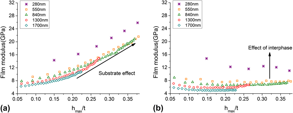
We end this study with a brief example of application of the models to experimental data of a polymer thin film on a stiff silica substrate. An added complication of thin polymer films is the presence of a significant regime of altered polymer behavior in the vicinity of the confining surface – thus the properties are altered from the bulk polymer properties in a gradient fashion from the substrate.Reference Watcharotone, Wood, Friedrich, Chen, Qiao, Putz and Brinson9,Reference Hamming, Qiao, Messersmith and Brinson42–Reference Rittigstein, Priestley, Broadbelt and Torkelson46 Here, data from Ref. Reference Watcharotone, Wood, Friedrich, Chen, Qiao, Putz and Brinson9 for films with different thickness are plotted in Fig. 8(a) using the original Oliver–Pharr model. The modulus increases both with increasing h c/t due to the substrate effect and with decreasing thickness due to the stiffer interphase polymer near the substrate. The overestimation of the film modulus is obvious, especially when h max/t is high. However, application of the Hay model to the data, as shown in Fig. 8(b), effectively removes the substrate effect, leaving the properties of the polymer interphase clearer to observe. These results are similar to the removal of the substrate effect using the direct FE approach as demonstrated in Eq. (32). With the help of enhanced understanding of different nanoindentation models, substrate effect can be removed from experimental data on compliant films such that a systematic knowledge on interphase in different film–substrate combinations is developed.
Experimental data of nanoindentation on PMMA film with various thicknesses in Ref. Reference Watcharotone, Wood, Friedrich, Chen, Qiao, Putz and Brinson9 are processed with the Oliver–Pharr model and results are shown in (a). The same data are processed with the Saha–Nix model to remove substrate effect in (b). After substrate effect is removed, thinner film still shows higher elastic modulus, which indicates the presence of interphase region in the PMMA film.

V. CONCLUSIONS
A direct comparison of several widely used nanoindentation models for thin film/substrate systems is presented in this study. FE simulations are performed to examine the validity of the different models over a range of experimental conditions, E f/E s and h max/t, with a focus on soft films on a stiff substrate. It is found that the performance of models in removal of the substrate effect varies especially as film compliance and indentation depth increase. The Saha–Nix and the Hay model are found to provide much more accurate analysis than the original Oliver–Pharr model. Although most of the nanoindentation models are developed based on the assumption that film is purely elastic, their performance is generally good with elastoplastic film. Subject to the validity regimes indicated in the results here, these models can effectively be used to remove the substrate effect analytically from experimental data without recourse to FE simulation for each case. The example of application of the models to experimental data of a glassy polymer film on silica is presented. The results demonstrate the importance of removing the substrate effect for compliant films and the possibility of using nanoindentation data to investigate the properties of the polymer interphase.
Supplementary Material
To view supplementary material for this article, please visit http://dx.doi.org/10.1557/jmr.2015.126.
ACKNOWLEDGMENTS
The authors gratefully acknowledge the financial support from the National Science Foundation (NSF grant CMMI-0928050) and the Office of Naval Research (ONR grant N00014-10-1-0043/P00007 and A12161//N000014-10-1-0244). Additionally, we acknowledge the helpful discussion with Ms. Jennifer Hay at Agilent Technology and Dr. Karl Putz, Dr. Charles Wood, and Xu Cheng in the department of Mechanical Engineering at Northwestern University. We also thank the critical attention of the reviewers who provided important comments and encouraged us to greatly improve the study.