1 Introduction
Orszag & Crow (Reference Orszag and Crow1970) considered the unsteady potential flow past the edge of a splitter plate with incompressible uniform flow on one side and stagnant fluid on the other side in the absence of external forcing. This simplest of inhomogeneous flows exhibits a concentrated vortex sheet in an unbounded inviscid fluid. They sought spatial growth, in contrast to the temporal growth more commonly sought in traditional stability theory, and left open the choice of Kutta condition, which determines how the sheet is attached to the plate. Crighton (Reference Crighton1972) studied the compressible version of Orszag & Crow’s problem and showed that spatial growth is unavoidable if a causal solution is required. In order to apply causality, Jones & Morgan (Reference Jones and Morgan1972) had considered an initial value problem in which linear theory is applied to acoustic radiation incident on a moving stream. The Helmholtz instability of an infinite vortex sheet must be present, along with an edge-scattered instability. Crighton & Leppington (Reference Crighton and Leppington1974), in the context of scattering of a point source of sound by a subsonic splitter plate, showed that causality can be enforced by allowing the frequency to be temporarily complex-valued. Use of the full-Kutta condition, in which the sheet has zero slope at its attachment, is thereby established. Daniels (Reference Daniels1978) confirmed this choice by including a triple-deck structure to demonstrate that a full-Kutta condition solution can be matched to a viscous inner solution but a no-Kutta condition cannot do likewise. Crighton (Reference Crighton1985) reviewed the application of Kutta conditions to a much wider range of flow problems than considered here. Peake (Reference Peake1994) considered another model problem, namely the flow resulting from the interaction between the trailing edge of a supersonic splitter plate and sound waves incident on the trailing edge from upstream. This is essentially the supersonic version of Jones & Morgan’s subsonic study. More recently, Samanta & Freund (Reference Samanta and Freund2008) noted that accepted practice is to use a full-Kutta condition, for which Bechert & Pfizenmaier (Reference Bechert and Pfizenmaier1975) provided experimental support. Rabchuk (Reference Rabchuk2000) identified trailing edge receptivity as disturbances converted into flow instabilities at the trailing edge, where the pressure is singular, in a mixing layer or wake. Triple-deck theory achieves theoretical consistency and gives clear physical justification for the unsteady Kutta condition, which accounts implicitly for viscosity but is inappropriate for the flow structure.
The splitter plate geometry permits solution via the Fourier transform. A natural question to consider is the effect of the local geometry of the trailing edge on the flow characteristics. The usual Kutta condition suggests that any sharp (non-reentrant) corner should lead to similar exponential growth but in the absence of other solutions to the problem, quantitative results are not known. The driving force behind the original work of Orszag & Crow (Reference Orszag and Crow1970) and subsequently of Crighton (Reference Crighton1972) and Crighton & Leppington (Reference Crighton and Leppington1974) was fundamentally the instability of the vortex sheet. The critical contribution of Crighton (Reference Crighton1972) was the explanation of the spatial growth. As a result we focus here on the instability. The full solution is obtained from the present formulation, but is not pursued computationally, as this would be lengthy and unmanageable. In addition the solution would be dominated by the instability, so that the extra work would be irrelevant. The finite-thickness unbounded shear layer is inviscidly unstable, with a short-wavelength cutoff. Hence the unphysical short-wavelength instability of the vortex sheet (Kelvin–Helmholtz instability) is not a problem and the present calculation is useful.
The paper is structured as follows. Section 2 formulates the problem: a uniform inviscid stream on one side of a rigid right-angled wedge is separated by a vortex sheet from stagnant inviscid fluid in the fourth quadrant. Unsteady potential flow is forced by an oscillatory doublet placed in the stream alongside the rigid quadrant. The resultant pressure forcing at the sheet is translated, by use of Mellin transforms, into a second-order functional difference equation system of period 2, which is equivalent to a first-order equation of period 4. The corresponding simpler equations for the semi-infinite plate have periods 2 and unity respectively and, for illustrative purposes, are solved in § 3 by each of two distinct methods. The second of these forms the basis of the
 $90^{\circ }$
trailing edge solution given in § 4. Its construction requires both the solution of the homogeneous difference equation of period 4 and the embedding of an inhomogeneous solution of period unity. The former uses the Barnes double Gamma function (Barnes Reference Barnes1899), ably described by Lawrie & King (Reference Lawrie and King1994), whose relevant results are listed in appendix A. The embedding exploits the fourth roots
 $(\pm 1\pm \text{i})$
of
 $-4$
to derive suitable functions of period unity. The four unknown constants are determined by eliminating poles within the strip of regularity. Causality is enforced by selecting a particular phase of the temporarily complex-valued frequency, whence the Helmholtz instability is shown to be present. Finally § 5 describes our conclusions. Some mathematical details are presented in appendix A.
2 Formulation
Consider incompressible, inviscid fluid in the three-quadrant region
 $r>0$
,
 $-\unicode[STIX]{x03C0}/2<\unicode[STIX]{x1D703}<\unicode[STIX]{x03C0}$
bounded by rigid walls, and suppose that a vortex sheet at
 $\unicode[STIX]{x1D703}=0$
is created by an imposed streaming flow
 $U\boldsymbol{e}_{x}$
in the half-space
 $y>0$
(region 1, with region 2 corresponding to
 $y<0$
). Assume that the perturbed flow
 $$\begin{eqnarray}\displaystyle & \displaystyle U\boldsymbol{e}_{x}+\unicode[STIX]{x1D735}\unicode[STIX]{x1D719}_{1}(x,y)\text{e}^{\text{i}kUt}\quad (-\infty <x<\infty ,y>0), & \displaystyle\end{eqnarray}$$
 $$\begin{eqnarray}\displaystyle & \displaystyle \unicode[STIX]{x1D735}\unicode[STIX]{x1D719}_{2}(x,y)\text{e}^{\text{i}kUt}\quad (0<x<\infty ,y<0), & \displaystyle\end{eqnarray}$$
 $$\begin{eqnarray}\displaystyle \unicode[STIX]{x1D6FB}^{2}\unicode[STIX]{x1D719}_{1}=0,\quad \unicode[STIX]{x1D6FB}^{2}\unicode[STIX]{x1D719}_{2}=0, & & \displaystyle\end{eqnarray}$$
in regions (1) and (2) respectively, the wall conditions are
 $$\begin{eqnarray}\displaystyle \frac{\unicode[STIX]{x2202}\unicode[STIX]{x1D719}_{1}}{\unicode[STIX]{x2202}y}(x,0)=0\,(x<0),\quad \frac{\unicode[STIX]{x2202}\unicode[STIX]{x1D719}_{2}}{\unicode[STIX]{x2202}x}(0,y)=0\,(y<0), & & \displaystyle\end{eqnarray}$$
the pressure is continuous when
 $$\begin{eqnarray}\displaystyle \text{i}k\unicode[STIX]{x1D719}_{1}(x,0)+\frac{\unicode[STIX]{x2202}\unicode[STIX]{x1D719}_{1}}{\unicode[STIX]{x2202}x}(x,0)=\text{i}k\unicode[STIX]{x1D719}_{2}(x,0)\quad (x>0), & & \displaystyle\end{eqnarray}$$
and the kinematic conditions, involving the interface displacement
 $\unicode[STIX]{x1D702}(x)\text{e}^{\text{i}kUt}$
, are
 $$\begin{eqnarray}\displaystyle \text{i}kU\unicode[STIX]{x1D702}+U\frac{\unicode[STIX]{x2202}\unicode[STIX]{x1D702}}{\unicode[STIX]{x2202}x}=\frac{\unicode[STIX]{x2202}\unicode[STIX]{x1D719}_{1}}{\unicode[STIX]{x2202}y}(x,0),\quad \text{i}kU\unicode[STIX]{x1D702}=\frac{\unicode[STIX]{x2202}\unicode[STIX]{x1D719}_{2}}{\unicode[STIX]{x2202}y}(x,0)\quad (x>0). & & \displaystyle\end{eqnarray}$$
If the forcing disturbance is described by the potential
 $\unicode[STIX]{x1D713}_{1}$
in region (1), then the potentials
 $$\begin{eqnarray}\displaystyle & \displaystyle \unicode[STIX]{x1D719}_{1}(x,y)+\unicode[STIX]{x1D713}_{1}(x,y)+\unicode[STIX]{x1D713}_{1}(x,-y)\quad (y>0), & \displaystyle\end{eqnarray}$$
 $$\begin{eqnarray}\displaystyle & \displaystyle \unicode[STIX]{x1D719}_{2}(x,y)\quad (y<0), & \displaystyle\end{eqnarray}$$
 $$\begin{eqnarray}\displaystyle \left(\text{i}k+\frac{\unicode[STIX]{x2202}}{\unicode[STIX]{x2202}x}\right)2\unicode[STIX]{x1D713}_{1}(x,0), & & \displaystyle\end{eqnarray}$$
from which we deduce that only pressure jump forcing need be considered here. The ‘image’ structure is made apparent by the acoustic solution given by Crighton & Leppington (Reference Crighton and Leppington1974) for the semi-infinite plate.
For a convenient and fundamental forcing, upstream of the vortex sheet, we set
 $$\begin{eqnarray}\displaystyle \unicode[STIX]{x1D713}_{1}(x,y)=\frac{Ur_{0}}{2\unicode[STIX]{x03C0}k}\frac{(x+x_{0})\cos \unicode[STIX]{x1D712}+(y-y_{0})\sin \unicode[STIX]{x1D712}}{(x+x_{0})^{2}+(y-y_{0})^{2}}\quad (x_{0},y_{0}>0), & & \displaystyle\end{eqnarray}$$
in which the angle
 $\unicode[STIX]{x1D712}$
allows the dipole at
 $(-x_{0},y_{0})=r_{0}(-\text{cos}\,\unicode[STIX]{x1D709}_{0},\sin \unicode[STIX]{x1D709}_{0})$
to be arbitrarily oriented. Then the flow is forced by the pressure condition
 $$\begin{eqnarray}\displaystyle \hspace{-15.00002pt}\unicode[STIX]{x1D719}_{2}(x,0)-\unicode[STIX]{x1D719}_{1}(x,0)-\frac{1}{\text{i}k}\frac{\unicode[STIX]{x2202}\unicode[STIX]{x1D719}_{1}}{\unicode[STIX]{x2202}x}(x,0) & = & \displaystyle \frac{Ur_{0}}{2\unicode[STIX]{x03C0}k}\left(1+\frac{1}{\text{i}k}\frac{\unicode[STIX]{x2202}}{\unicode[STIX]{x2202}x_{0}}\right)\nonumber\\ \displaystyle & & \displaystyle \times \!\left[\frac{\text{e}^{\text{i}\unicode[STIX]{x1D712}}}{x+x_{0}-\text{i}y_{0}}+\frac{\text{e}^{-\text{i}\unicode[STIX]{x1D712}}}{x+x_{0}+\text{i}y_{0}}\right]\quad (x>0).\end{eqnarray}$$
In view of (2.2) and the given geometry, define the usual Mellin transform
 $$\begin{eqnarray}\displaystyle \unicode[STIX]{x1D6F7}(s,\unicode[STIX]{x1D703})=\int _{0}^{\infty }\unicode[STIX]{x1D719}(r,\unicode[STIX]{x1D703})r^{s-1}\,\text{d}r, & & \displaystyle\end{eqnarray}$$
where
 $0<\text{Re}(s)<1$
is required for the transform to exist. Then the transformed conditions at
 $\unicode[STIX]{x1D703}=0$
are
 $$\begin{eqnarray}\displaystyle & \displaystyle \frac{\unicode[STIX]{x2202}\unicode[STIX]{x1D6F7}_{1}}{\unicode[STIX]{x2202}\unicode[STIX]{x1D703}}(s,0)=\frac{\unicode[STIX]{x2202}\unicode[STIX]{x1D6F7}_{2}}{\unicode[STIX]{x2202}\unicode[STIX]{x1D703}}(s,0)-\frac{s}{\text{i}k}\frac{\unicode[STIX]{x2202}\unicode[STIX]{x1D6F7}_{2}}{\unicode[STIX]{x2202}\unicode[STIX]{x1D703}}(s-1,0), & \displaystyle\end{eqnarray}$$
 $$\begin{eqnarray}\displaystyle & \displaystyle \unicode[STIX]{x1D6F7}_{2}(s,0)-\unicode[STIX]{x1D6F7}_{1}(s,0)+\frac{s-1}{\text{i}k}\unicode[STIX]{x1D6F7}_{1}(s-1,0)=\frac{Ur_{0}}{\unicode[STIX]{x03C0}}\frac{\unicode[STIX]{x1D6E4}(s)}{k^{s}}F(s), & \displaystyle\end{eqnarray}$$
 $\text{Re}(s)<1$
,
 $$\begin{eqnarray}\displaystyle F(s) & = & \displaystyle \left(1+\frac{1}{\text{i}k}\frac{\unicode[STIX]{x2202}}{\unicode[STIX]{x2202}x_{0}}\right)\frac{\unicode[STIX]{x1D6E4}(1-s)}{2}\left[\frac{\text{e}^{\text{i}\unicode[STIX]{x1D712}}}{(kr_{0}\text{e}^{-\text{i}\unicode[STIX]{x1D709}_{0}})^{1-s}}+\frac{\text{e}^{-\text{i}\unicode[STIX]{x1D712}}}{(kr_{0}\text{e}^{\text{i}\unicode[STIX]{x1D709}_{0}})^{1-s}}\right]\nonumber\\ \displaystyle & = & \displaystyle \frac{\unicode[STIX]{x1D6E4}(1-s)}{2(kr_{0})^{2-s}}\left\{\text{e}^{\text{i}[\unicode[STIX]{x1D712}+(2-s)\unicode[STIX]{x1D709}_{0}]}[k(x_{0}-\text{i}y_{0})-\text{i}(s-1)]\right.\nonumber\\ \displaystyle & & \displaystyle \left.+\,\text{e}^{-\text{i}[\unicode[STIX]{x1D712}+(2-s)\unicode[STIX]{x1D709}_{0}]}[k(x_{0}+\text{i}y_{0})-\text{i}(s-1)]\right\}.\end{eqnarray}$$
Dimensional coordinates
 $x$
,
 $y$
,
 $r$
are retained so that the Mellin transforms depend on
 $k$
.
Laplace’s equation (2.2) requires
 $\unicode[STIX]{x1D6F7}_{1}$
,
 $\unicode[STIX]{x1D6F7}_{2}$
to be linear combinations of
 $\cos s\unicode[STIX]{x1D703}$
,
 $\sin s\unicode[STIX]{x1D703}$
and then the conditions at the rigid boundaries are satisfied by writing
 $$\begin{eqnarray}\displaystyle \unicode[STIX]{x1D6F7}_{1} & = & \displaystyle Ur_{0}\frac{\unicode[STIX]{x1D6E4}(s)}{\unicode[STIX]{x03C0}k^{s}}\unicode[STIX]{x1D6FC}(s)\frac{\cos s(\unicode[STIX]{x03C0}-\unicode[STIX]{x1D703})}{\cos s\unicode[STIX]{x03C0}},\end{eqnarray}$$
 $$\begin{eqnarray}\displaystyle \unicode[STIX]{x1D6F7}_{2} & = & \displaystyle Ur_{0}\frac{\unicode[STIX]{x1D6E4}(s)}{\unicode[STIX]{x03C0}k^{s}}\unicode[STIX]{x1D6FE}(s)\frac{\cos s(\unicode[STIX]{x03C0}+\unicode[STIX]{x1D703})+\cos s\unicode[STIX]{x1D703}}{\cos s\unicode[STIX]{x03C0}},\end{eqnarray}$$
 $$\begin{eqnarray}\displaystyle N(s)=\int _{0}^{\infty }\unicode[STIX]{x1D702}(x)x^{s-1}\,\text{d}x=\text{i}r_{0}\frac{\unicode[STIX]{x1D6E4}(s)}{\unicode[STIX]{x03C0}k^{s}}\unicode[STIX]{x1D6FE}(s-1)\tan s\unicode[STIX]{x03C0}. & & \displaystyle\end{eqnarray}$$
So the interface conditions (2.11a ) yield, in matrix form,
 $$\begin{eqnarray}\displaystyle \left[\begin{array}{@{}c@{}}\unicode[STIX]{x1D6FE}(s-1)\\ \unicode[STIX]{x1D6FC}(s-1)\end{array}\right]-\text{i}\left[\begin{array}{@{}cc@{}}1 & 1\\ -(1+\sec s\unicode[STIX]{x03C0}) & 1\end{array}\right]\left[\begin{array}{@{}c@{}}\unicode[STIX]{x1D6FE}(s)\\ \unicode[STIX]{x1D6FC}(s)\end{array}\right]=\text{i}F(s)\left[\begin{array}{@{}c@{}}0\\ 1\end{array}\right], & & \displaystyle\end{eqnarray}$$
in which the matrix has period
 $2$
as a function of
 $s$
. Therefore we have to solve a second-order functional difference equation system of period
 $2$
, which is equivalent to a first-order system of period
 $4$
.
To identify the required strip of regularity, first note that the velocity components have Mellin transforms
 $$\begin{eqnarray}\displaystyle & \displaystyle \int _{0}^{\infty }\frac{\unicode[STIX]{x2202}\unicode[STIX]{x1D719}_{j}}{\unicode[STIX]{x2202}r}(r,\unicode[STIX]{x1D703})r^{s-1}\,\text{d}r=-(s-1)\unicode[STIX]{x1D6F7}_{j}(s-1,\unicode[STIX]{x1D703}), & \displaystyle\end{eqnarray}$$
 $$\begin{eqnarray}\displaystyle & \displaystyle \int _{0}^{\infty }\frac{1}{r}\frac{\unicode[STIX]{x2202}\unicode[STIX]{x1D719}_{j}}{\unicode[STIX]{x2202}\unicode[STIX]{x1D703}}(r,\unicode[STIX]{x1D703})r^{s-1}\,\text{d}r=\frac{\unicode[STIX]{x2202}\unicode[STIX]{x1D6F7}_{j}}{\unicode[STIX]{x2202}\unicode[STIX]{x1D703}}(s-1,\unicode[STIX]{x1D703}). & \displaystyle\end{eqnarray}$$
 $$\begin{eqnarray}\displaystyle N(s)=\frac{1}{\text{i}kU}\frac{\unicode[STIX]{x2202}\unicode[STIX]{x1D6F7}_{2}}{\unicode[STIX]{x2202}\unicode[STIX]{x1D703}}(s-1,0). & & \displaystyle\end{eqnarray}$$
These functions involve
 $\unicode[STIX]{x1D6FE}(s-1)$
and
 $\unicode[STIX]{x1D6FC}(s-1)$
, whose regularity in
 $0<\text{Re}(s)<1$
is achieved by ensuring the regularity of
 $\unicode[STIX]{x1D6FE}(s)$
and
 $\unicode[STIX]{x1D6FC}(s)$
in
 $-1<\text{Re}(s)<0$
.
3 The semi-infinite plate
We use this simpler problem first considered by Orszag & Crow (Reference Orszag and Crow1970) to demonstrate features and structure of the solution that we construct below for the rigid quadrant problem. With region (2) extended to
 $\unicode[STIX]{x1D703}=-\unicode[STIX]{x03C0}$
, the second wall condition is replaced by
 $$\begin{eqnarray}\displaystyle \frac{\unicode[STIX]{x2202}\unicode[STIX]{x1D719}_{2}}{\unicode[STIX]{x2202}y}(x,0)=0\quad (x<0). & & \displaystyle\end{eqnarray}$$
The conditions at the rigid plate
 $\unicode[STIX]{x1D703}=\pm \unicode[STIX]{x03C0}$
are satisfied by modifying the second condition in (2.13b
) and writing
 $$\begin{eqnarray}\displaystyle \unicode[STIX]{x1D6F7}_{1}=Ur_{0}\frac{\unicode[STIX]{x1D6E4}(s)}{\unicode[STIX]{x03C0}k^{s}}\unicode[STIX]{x1D6FC}(s)\frac{\cos s(\unicode[STIX]{x03C0}-\unicode[STIX]{x1D703})}{\cos s\unicode[STIX]{x03C0}},\quad \unicode[STIX]{x1D6F7}_{2}=Ur_{0}\frac{\unicode[STIX]{x1D6E4}(s)}{\unicode[STIX]{x03C0}k^{s}}\unicode[STIX]{x1D6FE}(s)\frac{\cos s(\unicode[STIX]{x03C0}+\unicode[STIX]{x1D703})}{\cos s\unicode[STIX]{x03C0}}, & & \displaystyle\end{eqnarray}$$
whence the interface conditions yield (2.14) and, in matrix form,
 $$\begin{eqnarray}\displaystyle \left[\begin{array}{@{}c@{}}\unicode[STIX]{x1D6FE}(s-1)\\ \unicode[STIX]{x1D6FC}(s-1)\end{array}\right]-\text{i}\left[\begin{array}{@{}cc@{}}1 & 1\\ -1 & 1\end{array}\right]\left[\begin{array}{@{}c@{}}\unicode[STIX]{x1D6FE}(s)\\ \unicode[STIX]{x1D6FC}(s)\end{array}\right]=\text{i}F(s)\left[\begin{array}{@{}c@{}}0\\ 1\end{array}\right]. & & \displaystyle\end{eqnarray}$$
The eigenvectors of the constant matrix facilitate the rearrangement of (3.3) as a pair of disjoint first-order equations,
 $$\begin{eqnarray}\displaystyle \unicode[STIX]{x1D6FC}(s-1)\pm \text{i}\unicode[STIX]{x1D6FE}(s-1)-(\text{i}\mp 1)[\unicode[STIX]{x1D6FC}(s)\pm \text{i}\unicode[STIX]{x1D6FE}(s)]=\text{i}F(s). & & \displaystyle\end{eqnarray}$$
Particular solutions of the form
 $$\begin{eqnarray}\displaystyle \unicode[STIX]{x1D6FC}(s)\pm \text{i}\unicode[STIX]{x1D6FE}(s)=\frac{1}{2\unicode[STIX]{x03C0}}\int _{\unicode[STIX]{x1D708}-\text{i}\infty }^{\unicode[STIX]{x1D708}+\text{i}\infty }F(u)I_{\pm }(u-s)\,\text{d}u\quad (\unicode[STIX]{x1D708}-1<\text{Re}(s)<\unicode[STIX]{x1D708}), & & \displaystyle\end{eqnarray}$$
exist provided that
 $$\begin{eqnarray}\displaystyle \int _{\unicode[STIX]{x1D708}-1-\text{i}\infty }^{\unicode[STIX]{x1D708}-1+\text{i}\infty }F(u)I_{\pm }(u-s+1)\,\text{d}u-(\text{i}\mp 1)\int _{\unicode[STIX]{x1D708}-\text{i}\infty }^{\unicode[STIX]{x1D708}+\text{i}\infty }F(u)I_{\pm }(u-s)\,\text{d}u=2\unicode[STIX]{x03C0}\text{i}F(s), & & \displaystyle\end{eqnarray}$$
which requires that
 $I_{\pm }(u-s+1)=(\text{i}\mp 1)I_{\pm }(u-s)$
with
 $I_{\pm }(u-s)$
regular in the strip
 $\unicode[STIX]{x1D708}-1<\text{Re}(s)<\unicode[STIX]{x1D708}$
except at
 $u=s$
where its residue is
 $(-\text{i}\pm 1)^{-1}$
. A suitable choice is
 $I_{\pm }(v)=\unicode[STIX]{x03C0}(-\text{i}\pm 1)^{v-1}/\sin \unicode[STIX]{x03C0}v$
, whence (3.4) has solution, in the strip
 $-1<\text{Re}(s)<0$
,
 $$\begin{eqnarray}\displaystyle \unicode[STIX]{x1D6FC}(s)\pm \text{i}\unicode[STIX]{x1D6FE}(s)=C_{\pm }(\text{i}\mp 1)^{-s}+\frac{1}{2}\int _{-\text{i}\infty }^{\text{i}\infty }\frac{F(u)}{\sin \unicode[STIX]{x03C0}(u-s)}(-\text{i}\pm 1)^{u-s-1}\,\text{d}u. & & \displaystyle\end{eqnarray}$$
The physically necessary elimination of the poles in
 $\unicode[STIX]{x1D6F7}_{1},\unicode[STIX]{x1D6F7}_{2}$
at
 $s=-1/2$
is achieved by setting
 $\unicode[STIX]{x1D6FE}(-1/2)=0=\unicode[STIX]{x1D6FC}(-1/2)$
. The second interface condition then eliminates the pole in
 $\unicode[STIX]{x1D6F7}_{2}$
at
 $s=-3/2$
, corresponding to applying the full-Kutta condition (tangential contact of the interface; see Daniels (Reference Daniels1978)). Thus, we choose
 $$\begin{eqnarray}\displaystyle C_{\pm }(\text{i}\mp 1)^{1/2}=-\frac{1}{2}\int _{-\text{i}\infty }^{\text{i}\infty }\frac{F(u)}{\cos \unicode[STIX]{x03C0}u}(-\text{i}\pm 1)^{u-1/2}\,\text{d}u. & & \displaystyle\end{eqnarray}$$
For
 $\unicode[STIX]{x1D6F7}_{1}$
and
 $\unicode[STIX]{x1D6F7}_{2}$
to be proper Mellin transforms, they must decay as
 $\text{Im}(s)\rightarrow \pm \infty$
within the strip of regularity. This can be achieved, as explained by Crighton & Leppington (Reference Crighton and Leppington1974) for the conjugate time dependence, by temporarily replacing
 $k$
by
 $k-\text{i}K$
in the complementary functions and requiring
 $(k-\text{i}K)(1+\text{i})$
and
 $(k-\text{i}K)(-1+\text{i})$
to have positive real parts. Inversion and the subsequent setting of
 $K$
to zero yields the solution. In particular, the term with
 $C_{+}$
generates the exponentially growing Helmholtz potentials
 $\unicode[STIX]{x1D719}_{2}^{H}$
,
 $\unicode[STIX]{x1D719}_{1}^{H}$
(Orszag & Crow Reference Orszag and Crow1970) given by
 $$\begin{eqnarray}\displaystyle & \displaystyle \unicode[STIX]{x1D719}_{1}^{H}=\text{i}Uh\exp [(1-\text{i})k(x+\text{i}y)]\quad (y>0), & \displaystyle\end{eqnarray}$$
 $$\begin{eqnarray}\displaystyle & \displaystyle \unicode[STIX]{x1D719}_{2}^{H}=Uh\exp [(1-\text{i})k(x-\text{i}y)]\quad (y<0). & \displaystyle\end{eqnarray}$$
 $k$
by
 $k_{0}\text{e}^{-\text{i}\unicode[STIX]{x03C0}\unicode[STIX]{x1D6FD}}k$
with
 $\unicode[STIX]{x03C0}/4<\unicode[STIX]{x1D6FD}<3\unicode[STIX]{x03C0}/4$
during the inversion and set
 $k=k_{0}$
(i.e.
 $\unicode[STIX]{x1D6FD}=0$
) in the final results.
We now rework the problem as an example of the following result. If the matrix
 $\unicode[STIX]{x1D63C}(s)$
has period
 $4$
and
 $\unicode[STIX]{x1D63C}(s)\unicode[STIX]{x1D63C}(s+1)\unicode[STIX]{x1D63C}(s+2)\unicode[STIX]{x1D63C}(s+3)=g(s)\unicode[STIX]{x1D644}$
, where
 $\unicode[STIX]{x1D644}$
denotes the identity matrix, then
 $g(s)$
has period
 $1$
and the system
 $$\begin{eqnarray}\displaystyle \boldsymbol{x}(s-1)-\unicode[STIX]{x1D63C}(s)\boldsymbol{x}(s)=f(s)\boldsymbol{c}, & & \displaystyle\end{eqnarray}$$
with
 $\boldsymbol{c}$
a constant vector, has solution
 $$\begin{eqnarray}\displaystyle \boldsymbol{x}(s) & = & \displaystyle \{\!\unicode[STIX]{x1D63C}(s+1)\unicode[STIX]{x1D63C}(s+2)\unicode[STIX]{x1D63C}(s+3)D(s)+\unicode[STIX]{x1D63C}(s+1)\unicode[STIX]{x1D63C}(s+2)D(s-1)\nonumber\\ \displaystyle & & \displaystyle +\,\unicode[STIX]{x1D63C}(s+1)D(s-2)+\unicode[STIX]{x1D644}D(s-3)\!\}\boldsymbol{c},\end{eqnarray}$$
provided
 $D(s)$
satisfies the difference equation
 $D(s-4)-g(s)D(s)=f(s)$
. Thus (3.3) has a solution of the form
 $$\begin{eqnarray}\displaystyle \left[\begin{array}{@{}c@{}}\unicode[STIX]{x1D6FE}(s)\\ \unicode[STIX]{x1D6FC}(s)\end{array}\right]=D(s)\left[\begin{array}{@{}c@{}}-2\text{i}\\ 2\text{i}\end{array}\right]+D(s-1)\left[\begin{array}{@{}c@{}}-2\\ 0\end{array}\right]+D(s-2)\left[\begin{array}{@{}c@{}}\text{i}\\ \text{i}\end{array}\right]+D(s-3)\left[\begin{array}{@{}c@{}}0\\ 1\end{array}\right], & & \displaystyle\end{eqnarray}$$
provided that
 $$\begin{eqnarray}\displaystyle D(s-4)+4D(s)=\text{i}F(s). & & \displaystyle\end{eqnarray}$$
The function
 $D(s)$
, of period
 $4$
, has the particular solution, constructed as in (3.7),
 $$\begin{eqnarray}\displaystyle \frac{1}{32}\int _{-\text{i}\infty }^{\text{i}\infty }2^{(u-s)/2}\frac{F(u)}{\sin \unicode[STIX]{x03C0}(u-s)/4}\,\text{d}u\quad \text{in }-4<\text{Re}(s)<0. & & \displaystyle\end{eqnarray}$$
The difference equation (3.13) of period
 $4$
has a complementary function that displays the fourth roots of
 $-4$
. Thus, in the strip
 $-4<\text{Re}(s)<0$
,
 $$\begin{eqnarray}\displaystyle D(s) & = & \displaystyle \frac{1}{16}\left\{C_{1}(1+\text{i})^{1-s}+C_{2}(-1+\text{i})^{1-s}+C_{3}(-1-\text{i})^{1-s}+C_{4}(1-\text{i})^{1-s}\vphantom{\int -\text{i}\infty ^{\text{i}\infty }}\right.\nonumber\\ \displaystyle & & \displaystyle \left.\!+\,\frac{1}{2}\int _{-\text{i}\infty }^{\text{i}\infty }2^{(u-s)/2}\frac{F(u)}{\sin \unicode[STIX]{x03C0}(u-s)/4}\,\text{d}u\right\}.\end{eqnarray}$$
Use of the identity
 $$\begin{eqnarray}\displaystyle \frac{2^{v/2}}{\sin \unicode[STIX]{x03C0}v/4}=\frac{(1+\text{i})^{v}+(-1+\text{i})^{v}+(-1-\text{i})^{v}+(1-\text{i})^{v}}{\sin \unicode[STIX]{x03C0}v} & & \displaystyle\end{eqnarray}$$
in (3.15) leads, in the strip
 $-1<\text{Re}(s)<0$
, to
 $$\begin{eqnarray}\displaystyle \hspace{-25.00003pt}\left[\begin{array}{@{}c@{}}\unicode[STIX]{x1D6FE}(s)\\ \unicode[STIX]{x1D6FC}(s)\end{array}\right] & = & \displaystyle -\frac{1}{2}\left\{C_{1}(1+\text{i})^{-s}\left[\begin{array}{@{}c@{}}\text{i}\\ 1\end{array}\right]+C_{2}(-1+\text{i})^{-s}\left[\begin{array}{@{}c@{}}-\text{i}\\ 1\end{array}\right]\right\}\nonumber\\ \displaystyle & & \displaystyle +\,\frac{1}{4}\int _{-\text{i}\infty }^{\text{i}\infty }\frac{F(u)}{\sin \unicode[STIX]{x03C0}(u-s)}\,\text{d}u\left\{(-1-\text{i})^{u-s-1}\left[\begin{array}{@{}c@{}}\text{i}\\ 1\end{array}\right]+(1-\text{i})^{u-s-1}\left[\begin{array}{@{}c@{}}-\text{i}\\ 1\end{array}\right]\right\},\end{eqnarray}$$
in agreement with (3.7). This result can be obtained by manipulation of the trigonometric functions in
 $$\begin{eqnarray}\displaystyle & & \displaystyle \left[\begin{array}{@{}c@{}}-2\text{i}\\ 2\text{i}\end{array}\right]\frac{1}{\sin \unicode[STIX]{x03C0}(u-s)/4}+\left[\begin{array}{@{}c@{}}-2\\ 0\end{array}\right]\frac{\sqrt{2}}{\sin \unicode[STIX]{x03C0}(u-s+1)/4}\nonumber\\ \displaystyle & & \displaystyle \quad +\left[\begin{array}{@{}c@{}}\text{i}\\ \text{i}\end{array}\right]\frac{2}{\sin \unicode[STIX]{x03C0}(u-s+2)/4}+\left[\begin{array}{@{}c@{}}0\\ 1\end{array}\right]\frac{2\sqrt{2}}{\sin \unicode[STIX]{x03C0}(u-s+3)/4}.\end{eqnarray}$$
To obtain this relation, we use the principal branch of the logarithm for the powers of
 $(\pm 1\pm \text{i})$
.
Computing the solution numerically, e.g. for
 $\unicode[STIX]{x1D702}(x)$
, is a two-step process. First we obtain
 $C_{1}$
and
 $C_{2}$
by enforcing the regularity condition
 $\unicode[STIX]{x1D6FE}(-1/2)=\unicode[STIX]{x1D6FC}(-1/2)=0$
in (3.17): this gives two equations. Then
 $\unicode[STIX]{x1D702}(x)$
can be found by computing the inverse Mellin transform of (2.14) using (3.17) to obtain
 $\unicode[STIX]{x1D6FE}(s-1)$
. We shall not carry out this programme here. Instead we concentrate on the exponentially growing contribution: this is the most interesting physically and also requires care in its calculation.
The homogeneous terms in
 $\unicode[STIX]{x1D702}(x)$
from (3.17) are related to the following Mellin transform (which does not seem to appear in standard references):
 $$\begin{eqnarray}\displaystyle \unicode[STIX]{x1D6E4}(s)\tan s\unicode[STIX]{x03C0}=\int _{0}^{\infty }\frac{2}{\sqrt{\unicode[STIX]{x03C0}}}F_{D}(\sqrt{r})r^{s-1}\,\text{d}r, & & \displaystyle\end{eqnarray}$$
in which
 $F_{D}(z)\equiv \text{e}^{-z^{2}}\int _{0}^{z}\text{e}^{t^{2}}\,\text{d}t$
is Dawson’s integral (Olver et al.
Reference Olver, Lozier, Boisvert and Clark2010). The solution can also be written in terms of error functions of imaginary arguments, as in Orszag & Crow (Reference Orszag and Crow1970, (4.4)). The growing homogeneous contribution to
 $\unicode[STIX]{x1D702}(x)$
comes from
 $$\begin{eqnarray}\frac{(1-\text{i})r_{0}}{2\unicode[STIX]{x03C0}}C_{2}[k(-1+\text{i})]^{-s}\unicode[STIX]{x1D6E4}(s)\tan s\unicode[STIX]{x03C0}.\end{eqnarray}$$
This does not have an inverse Mellin transform. However, the analytic continuation procedure of Crighton & Leppington (Reference Crighton and Leppington1974) corresponds to taking the inverse Mellin transform formally, using the standard scaling transformation for inverse Mellin transforms of
 $F_{D}(s)a^{-s}$
, which yields
 $$\begin{eqnarray}\displaystyle \unicode[STIX]{x1D702}(x)\sim \frac{(1-\text{i})r_{0}}{\unicode[STIX]{x03C0}^{3/2}}C_{2}F_{D}(\sqrt{(-1+\text{i})kx}), & & \displaystyle\end{eqnarray}$$
which grows exponentially downstream along the vortex sheet. The dominant behaviour of
 $\unicode[STIX]{x1D702}(x)$
for large
 $x$
can be obtained as
 $$\begin{eqnarray}\displaystyle \unicode[STIX]{x1D702}(x)\sim \frac{(1+\text{i})r_{0}}{2\unicode[STIX]{x03C0}}C_{2}\text{e}^{(1-\text{i})kx}. & & \displaystyle\end{eqnarray}$$
The amplitude of the Helmholtz mode is a function of
 $k$
,
 $U$
,
 $r_{0}$
,
 $\unicode[STIX]{x1D709}_{0}$
and
 $\unicode[STIX]{x1D712}$
. Of these variables,
 $U$
can be scaled out since the problem is linear, while
 $kr_{0}$
is the only non-dimensional length. There are hence three parameters:
 $kr_{0}$
and
 $\unicode[STIX]{x1D709}_{0}$
giving the polar coordinates of the dipole from the edge of the wedge and
 $\unicode[STIX]{x1D712}$
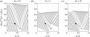
measuring the orientation of the dipole with respect to the horizontal. Figure 1 shows plots of the scaled amplitude of the Helmholtz mode,
 $(kr_{0})^{-3/2}|(1+\text{i})C_{2}|$
, as a function of
 $\unicode[STIX]{x1D712}$
for certain values of
 $kr_{0}$
and
 $0\leqslant \unicode[STIX]{x1D709}_{0}\leqslant \unicode[STIX]{x03C0}/2$
. The scaling
 $(kr_{0})^{-3/2}$
for both small and large values of
 $kr_{0}$
comes from the dominant singularity of the integrand in (3.17), which is at
 $1/2$
for
 $kr_{0}\ll 1$
and at
 $-1/2$
for
 $kr_{0}\gg 1$
. One can show that, up to the
 $kr_{0}$
factor, the integrals in (3.17) for large
 $kr_{0}$
differ by a factor of
 $\sqrt{2}$
compared to those for small
 $kr_{0}$
. This gives a factor of
 $\sqrt{2}$
difference between figures 1(a) and 1(c). The amplitude of the mode is a smoothly varying function with a minimum and maximum for each value of
 $\unicode[STIX]{x1D709}_{0}$
. For
 $\unicode[STIX]{x1D709}_{0}=0$
, the amplitude actually vanishes at
 $\unicode[STIX]{x1D712}=\unicode[STIX]{x03C0}/2$
.
Scaled amplitude
 $(kr_{0})^{-3/2}|(1+\text{i})C_{2}|$
. The range of
 $\unicode[STIX]{x1D709}_{0}$
is
 $(0,\unicode[STIX]{x03C0}/2)$
, with
 $\unicode[STIX]{x1D709}_{0}$
increasing in the direction of the arrow.

4 The right-angled wedge
4.1 Construction of solution
The repeated use of (2.15) yields
 $$\begin{eqnarray}\displaystyle \left[\begin{array}{@{}c@{}}\unicode[STIX]{x1D6FE}(s-2)\\ \unicode[STIX]{x1D6FC}(s-2)\end{array}\right]-\left[\begin{array}{@{}cc@{}}\sec s\unicode[STIX]{x03C0} & -2\\ 2 & -\sec s\unicode[STIX]{x03C0}\end{array}\right]\left[\begin{array}{@{}c@{}}\unicode[STIX]{x1D6FE}(s)\\ \unicode[STIX]{x1D6FC}(s)\end{array}\right]=\left[\begin{array}{@{}c@{}}-F(s)\\ \text{i}F(s-1)-F(s)\end{array}\right], & & \displaystyle\end{eqnarray}$$
which is a second-order system of period
 $2$
. We obtain a first-order equation of period
 $4$
by observing that the matrix in (2.15) allows a solution of the form
 $$\begin{eqnarray}\displaystyle \left[\begin{array}{@{}c@{}}\unicode[STIX]{x1D6FE}(s)\\ \unicode[STIX]{x1D6FC}(s)\end{array}\right] & = & \displaystyle D(s)(2-\sec s\unicode[STIX]{x03C0})\left[\begin{array}{@{}c@{}}-\text{i}\\ \text{i}\end{array}\right]+D(s-1)\left[\begin{array}{@{}c@{}}-2\\ -\sec s\unicode[STIX]{x03C0}\end{array}\right]\nonumber\\ \displaystyle & & \displaystyle +\,D(s-2)\left[\begin{array}{@{}c@{}}\text{i}\\ \text{i}\end{array}\right]+D(s-3)\left[\begin{array}{@{}c@{}}0\\ 1\end{array}\right],\end{eqnarray}$$
provided that
 $$\begin{eqnarray}\displaystyle D(s-4)+(4-\sec ^{2}s\unicode[STIX]{x03C0})D(s)=\text{i}F(s). & & \displaystyle\end{eqnarray}$$
We seek to reduce (4.3) to the form of (3.13) and hence introduce a function
 $H(s)$
that satisfies the difference equation
 $$\begin{eqnarray}\displaystyle H(s-4)=(1-{\textstyle \frac{1}{4}}\sec ^{2}s\unicode[STIX]{x03C0})H(s). & & \displaystyle\end{eqnarray}$$
It is shown in apendix A that a solution of (4.4) in integral form is given by
 $$\begin{eqnarray}\displaystyle H(s)=\exp \left\{2\int _{0}^{\infty }{\displaystyle \frac{\sinh {\displaystyle \frac{t}{4}}s\sinh ^{2}{\displaystyle \frac{t}{48}}}{\sinh {\displaystyle \frac{t}{2}}\sinh {\displaystyle \frac{t}{8}}}}{\displaystyle \frac{\text{d}t}{t}}\right\}, & & \displaystyle\end{eqnarray}$$
valid and analytic for
 $-7/3<\text{Re}(s)<7/3$
, which simply demonstrates that
 $H(s)H(-s)=1$
and
 $H(s)\rightarrow \text{e}^{\pm \text{i}\unicode[STIX]{x03C0}/144}$
as
 $\text{Im}(s)\rightarrow \pm \infty$
within this strip. See appendix A for the evaluation of the integral in (4.5). The pole structure of
 $H(s)$
is conveniently identified from its constituent Gamma functions which are shown in appendix A to yield
 $$\begin{eqnarray}\displaystyle H(s)=\mathop{\prod }_{m=0}^{\infty }\left[{\displaystyle \frac{\unicode[STIX]{x1D6E4}\left({\displaystyle \frac{5}{8}}+{\displaystyle \frac{s}{4}}+{\displaystyle \frac{m}{4}}\right)}{\unicode[STIX]{x1D6E4}\left({\displaystyle \frac{5}{8}}-{\displaystyle \frac{s}{4}}+{\displaystyle \frac{m}{4}}\right)}}\right]^{2}{\displaystyle \frac{\unicode[STIX]{x1D6E4}\left({\displaystyle \frac{2}{3}}-{\displaystyle \frac{s}{4}}+{\displaystyle \frac{m}{4}}\right)\unicode[STIX]{x1D6E4}\left({\displaystyle \frac{7}{12}}-{\displaystyle \frac{s}{4}}+{\displaystyle \frac{m}{4}}\right)}{\unicode[STIX]{x1D6E4}\left({\displaystyle \frac{2}{3}}+{\displaystyle \frac{s}{4}}+{\displaystyle \frac{m}{4}}\right)\unicode[STIX]{x1D6E4}\left({\displaystyle \frac{7}{12}}+{\displaystyle \frac{s}{4}}+{\displaystyle \frac{m}{4}}\right)}}. & & \displaystyle\end{eqnarray}$$
This defines
 $H(s)$
in the whole complex
 $s$
-plane with
 $H(0)=1$
. ‘Shifted’ values of
 $H(s)$
are obtained by noting, from (4.6) and the relation
 $\unicode[STIX]{x1D6E4}(z)\unicode[STIX]{x1D6E4}(1-z)=\unicode[STIX]{x03C0}\csc \unicode[STIX]{x03C0}z$
, that
 $$\begin{eqnarray}\displaystyle {\displaystyle \frac{H(s+1/2)}{H(s-1/2)}}={\displaystyle \frac{1+\cos s{\displaystyle \frac{\unicode[STIX]{x03C0}}{2}}}{\cos {\displaystyle \frac{\unicode[STIX]{x03C0}}{12}}+\cos s{\displaystyle \frac{\unicode[STIX]{x03C0}}{2}}}},\quad {\displaystyle \frac{H(s+1)}{H(s-1)}}={\displaystyle \frac{\left({\displaystyle \frac{1}{\sqrt{2}}}+\cos s{\displaystyle \frac{\unicode[STIX]{x03C0}}{2}}\right)^{2}}{\left({\displaystyle \frac{\sqrt{3}}{2}}+\cos s{\displaystyle \frac{\unicode[STIX]{x03C0}}{2}}\right)\left({\displaystyle \frac{1}{2}}+\cos s{\displaystyle \frac{\unicode[STIX]{x03C0}}{2}}\right)}}. & & \displaystyle \nonumber\\ \displaystyle & & \displaystyle\end{eqnarray}$$
Since the solution (4.2) includes values of
 $D(s)$
in the strip
 $-4<\text{Re}(s)<0$
when
 $-1<\text{Re}(s)<0$
, we note that
 $H(s+2)$
is regular in
 $-13/3<\text{Re}(s)<1/3$
and arrange (4.3) in the standard form
 $$\begin{eqnarray}\displaystyle \frac{D(s-4)}{H(s-2)}+4\frac{D(s)}{H(s+2)}=\frac{\text{i}F(s)}{H(s-2)}, & & \displaystyle\end{eqnarray}$$
because
 $H(s)$
is a solution of (4.4). We mimic the solution (3.15) of (3.13) in deducing that, in the strip
 $-4<\text{Re}(s)<0$
,
 $$\begin{eqnarray}\displaystyle \frac{D(s)}{H(s+2)} & = & \displaystyle \frac{1}{16}\left\{C_{1}(1+\text{i})^{1-s}+C_{2}(-1+\text{i})^{1-s}+C_{3}(-1-\text{i})^{1-s}+C_{4}(1-\text{i})^{1-s}\vphantom{\int _{-\text{i}\infty }^{\text{i}\infty }}\right.\nonumber\\ \displaystyle & & \displaystyle \left.+\,\frac{1}{2}\int _{-\text{i}\infty }^{\text{i}\infty }2^{(u-s)/2}\frac{F(u)\,\text{d}u}{H(u-2)\sin \unicode[STIX]{x03C0}(u-s)/4}\right\}.\end{eqnarray}$$
Then the substitution of (4.9) into (4.2) yields, in the strip
 $-1<\text{Re}(s)<0$
,
 $$\begin{eqnarray}\displaystyle & & \displaystyle \left[\begin{array}{@{}c@{}}\unicode[STIX]{x1D6FE}(s)\\ \unicode[STIX]{x1D6FC}(s)+\unicode[STIX]{x1D6FE}(s)\end{array}\right]=\frac{1}{16}\nonumber\\ \displaystyle & & \displaystyle \quad \times \!\left\{C_{1}(1+\text{i})^{1-s}\left[\begin{array}{@{}c@{}}-\text{i}(2-\sec s\unicode[STIX]{x03C0})H(s+2)-2(1+\text{i})H(s+1)-2H(s)\\ -(2+\sec s\unicode[STIX]{x03C0})(1+\text{i})H(s+1)-4H(s)+2(-1+\text{i})H(s-1)\end{array}\right]\right.\nonumber\\ \displaystyle & & \displaystyle \quad +\,C_{2}(-1+\text{i})^{1-s}\left[\begin{array}{@{}c@{}}-\text{i}(2-\sec s\unicode[STIX]{x03C0})H(s+2)-2(-1+\text{i})H(s+1)+2H(s)\\ -(2+\sec s\unicode[STIX]{x03C0})(-1+\text{i})H(s+1)+4H(s)+2(1+\text{i})H(s-1)\end{array}\right]\nonumber\\ \displaystyle & & \displaystyle \quad +\,C_{3}(-1-\text{i})^{1-s}\left[\begin{array}{@{}c@{}}-\text{i}(2-\sec s\unicode[STIX]{x03C0})H(s+2)-2(-1-\text{i})H(s+1)-2H(s)\\ -(2+\sec s\unicode[STIX]{x03C0})(-1-\text{i})H(s+1)-4H(s)+2(1-\text{i})H(s-1)\end{array}\right]\nonumber\\ \displaystyle & & \displaystyle \quad +\,C_{4}(1-\text{i})^{1-s}\left[\begin{array}{@{}c@{}}-\text{i}(2-\sec s\unicode[STIX]{x03C0})H(s+2)-2(1-\text{i})H(s+1)+2H(s)\\ -(2+\sec s\unicode[STIX]{x03C0})(1-\text{i})H(s+1)+4H(s)+2(-1-\text{i})H(s-1)\end{array}\right]\nonumber\\ \displaystyle & & \displaystyle \quad +\,\frac{1}{2}\int _{-\text{i}\infty }^{\text{i}\infty }\frac{F(u)\,\text{d}u}{H(u-2)\sin \unicode[STIX]{x03C0}(u-s)}\nonumber\\ \displaystyle & & \displaystyle \quad \times \!\left((1+\text{i})^{u-s}\left[\begin{array}{@{}c@{}}-\text{i}(2-\sec s\unicode[STIX]{x03C0})H(s+2)+2(1+\text{i})H(s+1)-2H(s)\\ (2+\sec s\unicode[STIX]{x03C0})(1+\text{i})H(s+1)-4H(s)-2(-1+\text{i})H(s-1)\end{array}\right]\right.\nonumber\\ \displaystyle & & \displaystyle \quad +\,(-1+\text{i})^{u-s}\left[\begin{array}{@{}c@{}}-\text{i}(2-\sec s\unicode[STIX]{x03C0})H(s+2)+2(-1+\text{i})H(s+1)+2H(s)\\ (2+\sec s\unicode[STIX]{x03C0})(-1+\text{i})H(s+1)+4H(s)-2(1+\text{i})H(s-1)\end{array}\right]\nonumber\\ \displaystyle & & \displaystyle \quad +\,(-1-\text{i})^{u-s}\left[\begin{array}{@{}c@{}}-\text{i}(2-\sec s\unicode[STIX]{x03C0})H(s+2)+2(-1-\text{i})H(s+1)-2H(s)\\ (2+\sec s\unicode[STIX]{x03C0})(-1-\text{i})H(s+1)-4H(s)-2(1-\text{i})H(s-1)\end{array}\right]\nonumber\\ \displaystyle & & \displaystyle \quad \left.\left.+\,(1-\text{i})^{u-s}\left[\begin{array}{@{}c@{}}-\text{i}(2-\sec s\unicode[STIX]{x03C0})H(s+2)+2(1-\text{i})H(s+1)+2H(s)\\ (2+\sec s\unicode[STIX]{x03C0})(1-\text{i})H(s+1)+4H(s)-2(-1-\text{i})H(s-1)\end{array}\right]\right)\right\}.\nonumber\\ \displaystyle & & \displaystyle\end{eqnarray}$$
4.2 Behaviour for large
 $\text{Im}(s)$

In the limits
 $\text{Im}(s)\rightarrow \pm \infty$
,
 $\sec s\unicode[STIX]{x03C0}\rightarrow 0$
and
 $H(s)\sim \text{e}^{\pm \text{i}\unicode[STIX]{x03C0}/144}$
and only values of
 $u$
near
 $s$
are significant in the integral. Thus (4.10) reduces to (3.17), as expected, because (4.2) and (4.3) then reduce to (3.3) and (3.13) respectively. The vectors multiplying
 $C_{3}$
,
 $C_{4}$
in (4.10) are
 $\mathbf{0}$
at leading order.
It is readily shown from (4.7) that, with
 $s=\unicode[STIX]{x1D709}+\text{i}\unicode[STIX]{x1D702}$
,
 $$\begin{eqnarray}\displaystyle \frac{H(s+1)}{H(s)}=1+O(\text{e}^{-|\unicode[STIX]{x1D702}|\unicode[STIX]{x03C0}/2})\quad \text{as }|\unicode[STIX]{x1D702}|\rightarrow \infty & & \displaystyle\end{eqnarray}$$
in the strip of regularity. Set
 $k=k_{0}\text{e}^{-\text{i}\unicode[STIX]{x1D6FD}}$
and note that
 $$\begin{eqnarray}\displaystyle \unicode[STIX]{x1D6E4}(\unicode[STIX]{x1D709}+\text{i}\unicode[STIX]{x1D702})=O(|\unicode[STIX]{x1D702}|^{\unicode[STIX]{x1D709}-1/2}\text{e}^{-|\unicode[STIX]{x1D702}|\unicode[STIX]{x03C0}/2})\quad \text{as }|\unicode[STIX]{x1D702}|\rightarrow \infty & & \displaystyle\end{eqnarray}$$
(Olver et al. Reference Olver, Lozier, Boisvert and Clark2010). Then, for exponential decay,
 $$\begin{eqnarray}\displaystyle & \displaystyle \frac{\unicode[STIX]{x1D6E4}(s)}{k^{s}(1+\text{i})^{s}}=O[|\unicode[STIX]{x1D702}|^{\unicode[STIX]{x1D709}-1/2}\text{e}^{-(\unicode[STIX]{x1D6FD}-\unicode[STIX]{x03C0}/4)\unicode[STIX]{x1D702}}\text{e}^{-|\unicode[STIX]{x1D702}|\unicode[STIX]{x03C0}/2}]\text{ requires }-\frac{\unicode[STIX]{x03C0}}{4}<\unicode[STIX]{x1D6FD}<\frac{3\unicode[STIX]{x03C0}}{4}, & \displaystyle\end{eqnarray}$$
 $$\begin{eqnarray}\displaystyle & \displaystyle \frac{\unicode[STIX]{x1D6E4}(s)}{k^{s}(-1+\text{i})^{s}}=O[|\unicode[STIX]{x1D702}|^{\unicode[STIX]{x1D709}-1/2}\text{e}^{-(\unicode[STIX]{x1D6FD}-3\unicode[STIX]{x03C0}/4)\unicode[STIX]{x1D702}}\text{e}^{-|\unicode[STIX]{x1D702}|\unicode[STIX]{x03C0}/2}]\text{ requires }\frac{\unicode[STIX]{x03C0}}{4}<\unicode[STIX]{x1D6FD}<\frac{5\unicode[STIX]{x03C0}}{4}, & \displaystyle\end{eqnarray}$$
 $$\begin{eqnarray}\displaystyle & \displaystyle \frac{\unicode[STIX]{x1D6E4}(s)\text{e}^{-|\unicode[STIX]{x1D702}|\unicode[STIX]{x03C0}/2}}{k^{s}(-1-\text{i})^{s}}=O[|\unicode[STIX]{x1D702}|^{\unicode[STIX]{x1D709}-1/2}\text{e}^{-(\unicode[STIX]{x1D6FD}+3\unicode[STIX]{x03C0}/4)\unicode[STIX]{x1D702}}\text{e}^{-|\unicode[STIX]{x1D702}|\unicode[STIX]{x03C0}}]\text{ requires }-\frac{7\unicode[STIX]{x03C0}}{4}<\unicode[STIX]{x1D6FD}<\frac{\unicode[STIX]{x03C0}}{4}, & \displaystyle\end{eqnarray}$$
 $$\begin{eqnarray}\displaystyle & \displaystyle \frac{\unicode[STIX]{x1D6E4}(s)\text{e}^{-|\unicode[STIX]{x1D702}|\unicode[STIX]{x03C0}/2}}{k^{s}(1-\text{i})^{s}}=O[|\unicode[STIX]{x1D702}|^{\unicode[STIX]{x1D709}-1/2}\text{e}^{-(\unicode[STIX]{x1D6FD}+\unicode[STIX]{x03C0}/4)\unicode[STIX]{x1D702}}\text{e}^{-|\unicode[STIX]{x1D702}|\unicode[STIX]{x03C0}}]\text{ requires }-\frac{5\unicode[STIX]{x03C0}}{4}<\unicode[STIX]{x1D6FD}<\frac{3\unicode[STIX]{x03C0}}{4}, & \displaystyle\end{eqnarray}$$
 $\unicode[STIX]{x1D6FD}=\unicode[STIX]{x03C0}/4$
ensures exponential decay in two cases, but in the other two relies on algebraic decay due to the additional
 $|\unicode[STIX]{x1D702}|^{\unicode[STIX]{x1D709}-1/2}$
factor with
 $-1<\unicode[STIX]{x1D709}<0$
in the strip of regularity.
4.3 Determination of the coefficients
The result (4.5) confirms that
 $H(s+2)$
,
 $H(s+1)$
,
 $H(s)$
and
 $H(s-1)$
have the common strip of analyticity
 $-4/3<\text{Re}(s)<1/3$
and therefore the only pole in (4.10) arises from
 $\sec s\unicode[STIX]{x03C0}$
. Inspection of the Mellin transforms, given by (2.13a
), (2.13b
), shows that
 $\unicode[STIX]{x1D6FE}(s)\sec s\unicode[STIX]{x03C0}$
and
 $\unicode[STIX]{x1D6FC}(s)\sec s\unicode[STIX]{x03C0}$
are regular at
 $s=-1/2$
, as required to eliminate terms of order
 $r^{1/2}$
from the small-
 $r$
expansions of
 $\unicode[STIX]{x1D719}_{2}$
and
 $\unicode[STIX]{x1D719}_{1}$
. As in the semi-infinite plate case, the first equation in (2.15) then implies that
 $\unicode[STIX]{x1D6FE}(-3/2)=0$
and hence, according to (2.14), satisfies the full-Kutta condition by proscribing an
 $x^{1/2}$
term in
 $\unicode[STIX]{x1D702}(x)$
.
The poles at
 $s=-1/2$
are eliminated by choice of the arbitrary constants,
 $C_{j}(1\leqslant j\leqslant 4)$
in (4.9) by demanding, in (4.2),
 $$\begin{eqnarray}\displaystyle \left.\begin{array}{@{}c@{}}D(-1/2)=0=D(-3/2),\quad {\displaystyle \frac{1}{\unicode[STIX]{x03C0}}}D^{\prime }(-1/2)+D(-5/2)=0,\\ {\displaystyle \frac{1}{\unicode[STIX]{x03C0}}}D^{\prime }(-3/2)=2\text{i}D(-5/2)+D(-7/2).\end{array}\right\} & & \displaystyle\end{eqnarray}$$
The first two of these conditions facilitate the evaluation of the derivatives without knowledge of
 $H^{\prime }(3/2),H^{\prime }(1/2)$
. It is readily deduced from (4.7) that
 $$\begin{eqnarray}\displaystyle \left.\begin{array}{@{}c@{}}H(1/2)=\sec {\displaystyle \frac{\unicode[STIX]{x03C0}}{24}}\quad H(-1/2)=\cos {\displaystyle \frac{\unicode[STIX]{x03C0}}{24}},\\ H(3/2)=\sec {\displaystyle \frac{\unicode[STIX]{x03C0}}{12}}\sec {\displaystyle \frac{\unicode[STIX]{x03C0}}{24}}\quad H(-3/2)=\cos {\displaystyle \frac{\unicode[STIX]{x03C0}}{12}}\cos {\displaystyle \frac{\unicode[STIX]{x03C0}}{24}}.\end{array}\right\} & & \displaystyle\end{eqnarray}$$
For algebraic brevity, write (4.9) as
 $$\begin{eqnarray}\displaystyle \frac{D(s)}{H(s+2)} & = & \displaystyle B_{1}(1+\text{i})^{-(s+1/2)}+B_{2}(-1+\text{i})^{-(s+1/2)}+B_{3}(-1-\text{i})^{-(s+1/2)}\nonumber\\ \displaystyle & & \displaystyle +\,B_{4}(1-\text{i})^{-(s+1/2)}+2^{-(s+1/2)/2}\int _{-\text{i}\infty }^{\text{i}\infty }\frac{G(u)\,\text{d}u}{\sin \unicode[STIX]{x03C0}(u-s)/4},\end{eqnarray}$$
where
 $$\begin{eqnarray}\displaystyle [C_{1},C_{2},C_{3},C_{4}]=16\left[B_{1}(1+\text{i})^{-3/2},B_{2}(-1+\text{i})^{-3/2},B_{3}(-1-\text{i})^{-3/2},B_{4}(1-\text{i})^{-3/2}\right], & & \displaystyle \nonumber\\ \displaystyle & & \displaystyle\end{eqnarray}$$
and
 $$\begin{eqnarray}\displaystyle F(u)=32\times 2^{-(u+1/2)/2}G(u)H(u-2). & & \displaystyle\end{eqnarray}$$
Then substitution of (4.15), (4.16) into (4.14) gives
 $$\begin{eqnarray}\displaystyle B_{1}+B_{2}+B_{3}+B_{4}+\int _{-\text{i}\infty }^{\text{i}\infty }\frac{G(u)\,\text{d}u}{\sin \unicode[STIX]{x03C0}(u+1/2)/4}=0, & & \displaystyle\end{eqnarray}$$
 $$\begin{eqnarray}\displaystyle & & \displaystyle B_{1}(1+\text{i})+B_{2}(-1+\text{i})+B_{3}(-1-\text{i})+B_{4}(1-\text{i})\nonumber\\ \displaystyle & & \displaystyle \quad +\,2^{1/2}\int _{-\text{i}\infty }^{\text{i}\infty }\frac{G(u)\,\text{d}u}{\sin \unicode[STIX]{x03C0}(u+3/2)/4}=0,\end{eqnarray}$$
 $$\begin{eqnarray}\displaystyle & & \displaystyle 2\cos \frac{\unicode[STIX]{x03C0}}{12}\left[B_{1}-B_{2}+B_{3}-B_{4}-\text{i}\int _{-\text{i}\infty }^{\text{i}\infty }\frac{G(u)\,\text{d}u}{\cos \unicode[STIX]{x03C0}(u+1/2)/4}\right]\nonumber\\ \displaystyle & & \displaystyle \quad =\frac{1}{4}\sec ^{2}\frac{\unicode[STIX]{x03C0}}{24}\left[B_{1}+3B_{2}-3B_{3}-B_{4}\right.\nonumber\\ \displaystyle & & \displaystyle \qquad \left.+\,\text{i}\int _{-\text{i}\infty }^{\text{i}\infty }\frac{G(u)\,\text{d}u}{\sin \unicode[STIX]{x03C0}(u+1/2)/4}\cot \unicode[STIX]{x03C0}(u+1/2)/4\right],\end{eqnarray}$$
 $$\begin{eqnarray}\displaystyle & & \displaystyle 4\left[-B_{1}+B_{2}-B_{3}+B_{4}+\text{i}\int _{-\text{i}\infty }^{\text{i}\infty }\frac{G(u)\,\text{d}u}{\cos \unicode[STIX]{x03C0}(u+1/2)/4}\right]\nonumber\\ \displaystyle & & \displaystyle \qquad +\,2\cos \frac{\unicode[STIX]{x03C0}}{12}\left[B_{1}(-1+\text{i})+B_{2}(1+\text{i})+B_{3}(1-\text{i})+B_{4}(-1-\text{i})\phantom{\int }\right.\nonumber\\ \displaystyle & & \displaystyle \qquad \left.+\,2^{1/2}\int _{-\text{i}\infty }^{\text{i}\infty }\frac{G(u)\,\text{d}u}{\cos \unicode[STIX]{x03C0}(u+3/2)/4}\right]\nonumber\\ \displaystyle & & \displaystyle \quad =\frac{1}{4}\sec ^{2}\frac{\unicode[STIX]{x03C0}}{24}\left[B_{1}(1-\text{i})+3B_{2}(1+\text{i})+3B_{3}(1-\text{i})+B_{4}(1+\text{i})\phantom{\int }\right.\nonumber\\ \displaystyle & & \displaystyle \qquad \left.+\,2^{1/2}\int _{-\text{i}\infty }^{\text{i}\infty }\frac{G(u)\,\text{d}u}{\sin \unicode[STIX]{x03C0}(u+3/2)/4}\cot \unicode[STIX]{x03C0}(u+3/2)/4\right].\end{eqnarray}$$
4.4 Calculation of the exponentially growing contribution
Once again we focus on the exponentially growing part of the solution, which comes from the terms containing
 $(-1\pm \text{i})^{-s}$
in (4.10). However, the term in
 $C_{3}$
is not needed because it vanishes to leading order as described in § 4.2. The computation of the displacement is more involved than for the half-plane case because of the presence of the function
 $H(s)$
. First (4.19)–(4.22) are solved for
 $B_{1}$
,
 $B_{2}$
,
 $B_{3}$
and
 $B_{4}$
. Note that the required integrals exist when
 $k$
is real. Then
 $C_{2}$
is obtained and used in (4.10) to obtain
 $\unicode[STIX]{x1D6FE}(s)$
. This is then used in the expression for
 $N(s)$
, which is inverse Mellin transformed. The condition
 $\unicode[STIX]{x1D6FD}=\unicode[STIX]{x03C0}/4$
is necessary for the exponentially growing terms to be Mellin transform. While we could carry out the inverse transform analytically for the semi-infinite plate, this is no longer possible here. To avoid having to use
 $\unicode[STIX]{x1D6FD}$
in the evaluation of the inverse Mellin transform, we proceed as follows.
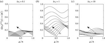
Scaled amplitude
 $(kr_{0})^{-3/2}|(1+\text{i})C_{2}|$
. The range of
 $\unicode[STIX]{x1D709}_{0}$
is
 $(0,\unicode[STIX]{x03C0}/2)$
, with
 $\unicode[STIX]{x1D709}_{0}$
increasing in the direction of the arrow.

We write for the Mellin transform of the growing homogeneous solution involving
 $C_{2}$
 $$\begin{eqnarray}\displaystyle \unicode[STIX]{x1D6FE}_{H}(s-1)=-\frac{\text{i}}{8}C_{2}(-1+\text{i})^{-s}H(s)[4-4\text{i}+l(s)], & & \displaystyle\end{eqnarray}$$
where
 $$\begin{eqnarray}\displaystyle l(s)=-2+2\text{i}-\text{i}(2+\sec s\unicode[STIX]{x03C0})\frac{H(s+1)}{H(s)}+2r_{-}(s)\frac{H(s-1)}{H(s)} & & \displaystyle\end{eqnarray}$$
decays as
 $\text{Im}(s)\rightarrow \infty$
. Our aim is to separate the inverse Mellin transform of
 $N(s)$
into two parts: one that can be done analytically and the other which has a Mellin transform for
 $\unicode[STIX]{x1D6FD}=0$
. Since
 $H(s)\sim \text{e}^{\pm \text{i}\unicode[STIX]{x03C0}/144}$
as
 $\text{Im}(s)\rightarrow \pm \infty$
, we can decompose
 $H(s)\tan s\unicode[STIX]{x03C0}$
as
 $$\begin{eqnarray}\displaystyle H(s)\tan s\unicode[STIX]{x03C0} & = & \displaystyle [H(s)\tan s\unicode[STIX]{x03C0}-\cos (\unicode[STIX]{x03C0}/144)\tan s\unicode[STIX]{x03C0}+\sin (\unicode[STIX]{x03C0}/144)]\nonumber\\ \displaystyle & & \displaystyle +\,\cos (\unicode[STIX]{x03C0}/144)\tan s\unicode[STIX]{x03C0}-\sin (\unicode[STIX]{x03C0}/144)=H_{1}(s)+H_{2}(s).\end{eqnarray}$$
As
 $\text{Im}(s)\rightarrow \pm \infty ,\,H_{1}(s)$
decays exponentially. The Mellin transform of the exponentially growing part of the interface displacement reduces to two parts:
 $$\begin{eqnarray}\displaystyle N_{H}(s)=N(s)=\frac{2r_{0}}{\unicode[STIX]{x03C0}k^{s}}C_{2}(-1+\text{i})^{-s}\unicode[STIX]{x1D6E4}(s)[H_{1}(s)+H_{2}(s)][4-4\text{i}+l(s)]. & & \displaystyle\end{eqnarray}$$
The growing part comes from the
 $H_{2}(s)(4-4\text{i})$
term and can be carried out by hand, as in (3.22), giving
 $$\begin{eqnarray}\displaystyle \unicode[STIX]{x1D702}(x)\sim \frac{2r_{0}}{\unicode[STIX]{x03C0}}C_{2}(4-4\text{i})\left[\cos (\unicode[STIX]{x03C0}/144)\frac{2}{\sqrt{\unicode[STIX]{x03C0}}}F_{D}(\sqrt{(-1+\text{i})kx})-\sin (\unicode[STIX]{x03C0}/144)\text{e}^{(1-\text{i})kx}\right]. & & \displaystyle \nonumber\\ \displaystyle & & \displaystyle\end{eqnarray}$$
Figure 2 shows plots of the scaled amplitude of the Helmholtz mode,
 $(kr_{0})^{-3/2}|(1+\text{i})C_{2}|$
, as a function of
 $\unicode[STIX]{x1D712}$
for certain values of
 $kr_{0}$
and
 $0\leqslant \unicode[STIX]{x1D709}_{0}\leqslant \unicode[STIX]{x03C0}/2$
. The scaling
 $(kr_{0})^{-3/2}$
persists for both small and large values of
 $kr_{0}$
. The amplitude of the mode is once again smoothly varying, vanishing at
 $\unicode[STIX]{x1D712}=\unicode[STIX]{x03C0}/2$
when
 $\unicode[STIX]{x1D709}_{0}=1$
, but varies more than for the semi-infinite plate. In particular the similarity between small and large
 $kr_{0}$
has gone, since
 $H(s)$
differs between
 $s=-1/2$
and
 $s=1/2$
. For large
 $kr_{0}$
, the largest amplitude is found for values of
 $\unicode[STIX]{x1D712}$
around
 $3\unicode[STIX]{x03C0}/4$
.
5 Conclusion
We have obtained the linearised evolution of the vortex sheet behind a right-angled wedge using the Mellin transform. This leads to a difference equation that can be solved using an appropriate integral representation. The fourth roots of
 $-4$
lead to complementary functions whose amplitudes are fixed by regularity conditions for the Mellin transform corresponding to the full-Kutta condition at the corner. For the semi-infinite plate, the amplitude of the single Helmholtz mode for the vortex sheet displacement can be obtained in analytic form: applying the necessary Mellin shift theorem involves an implicit use of the analytic continuation procedure discussed by Crighton & Leppington (Reference Crighton and Leppington1974). For the right-angled wedge, this procedure requires breaking up the Mellin transform into different contributions, one of which has a similar form and can be computed explicitly. In both cases, the amplitude of the growing mode is a function of the governing parameter of the problem (vanishing when the dipole has vertical orientation and lies along the
 $x$
-axis), with the form
 $\exp [(1-\text{i})kx]$
for
 $x\gg 1$
.
Acknowledgements
The authors gratefully acknowledge helpful discussions with E. J. Kerschen and N. Peake. This study was suggested by David Crighton, to whose memory the article is dedicated.
Appendix A. Homogeneous solution
The bracketed function in (4.4) has the factorization
 $$\begin{eqnarray}\displaystyle 1-{\displaystyle \frac{1}{4}}\sec ^{2}s\unicode[STIX]{x03C0}={\displaystyle \frac{\cos 2s\unicode[STIX]{x03C0}+{\displaystyle \frac{1}{2}}}{2\cos ^{2}s\unicode[STIX]{x03C0}}}={\displaystyle \frac{\cos \left(s-{\displaystyle \frac{1}{6}}\right)\unicode[STIX]{x03C0}\cos \left(s+{\displaystyle \frac{1}{6}}\right)\unicode[STIX]{x03C0}}{\cos ^{2}s\unicode[STIX]{x03C0}}}. & & \displaystyle\end{eqnarray}$$
Equations of this type are solved by Lawrie & King (Reference Lawrie and King1994) in terms of the Barnes double Gamma function (Barnes Reference Barnes1899) defined by
 $$\begin{eqnarray}\displaystyle G(z+1,\unicode[STIX]{x1D6FF})=\unicode[STIX]{x1D6E4}\left(\frac{z}{\unicode[STIX]{x1D6FF}}\right)G(z,\unicode[STIX]{x1D6FF}),\quad G(1,\unicode[STIX]{x1D6FF})=1. & & \displaystyle\end{eqnarray}$$
For earlier examples, see Williams (Reference Williams1959) and Lawrie (Reference Lawrie1990). Thus
 $$\begin{eqnarray}\displaystyle & \displaystyle \sin \left(\frac{\unicode[STIX]{x03C0}z}{\unicode[STIX]{x1D6FF}}\right)=\frac{\unicode[STIX]{x03C0}G(z,\unicode[STIX]{x1D6FF})G(\unicode[STIX]{x1D6FF}-z,\unicode[STIX]{x1D6FF})}{G(1+z,\unicode[STIX]{x1D6FF})G(1+\unicode[STIX]{x1D6FF}-z,\unicode[STIX]{x1D6FF})}, & \displaystyle\end{eqnarray}$$
 $$\begin{eqnarray}\displaystyle & \displaystyle \cos \left(\frac{\unicode[STIX]{x03C0}z}{\unicode[STIX]{x1D6FF}}\right)=\frac{\unicode[STIX]{x03C0}G(\unicode[STIX]{x1D6FF}/2+z,\unicode[STIX]{x1D6FF})G(\unicode[STIX]{x1D6FF}/2-z,\unicode[STIX]{x1D6FF})}{G(1+\unicode[STIX]{x1D6FF}/2+z,\unicode[STIX]{x1D6FF})G(1+\unicode[STIX]{x1D6FF}/2-z,\unicode[STIX]{x1D6FF})}. & \displaystyle\end{eqnarray}$$
 $s=4S$
,
 $E(s)=f(S)$
, the difference equation (4.4) may be written as
 $$\begin{eqnarray}\displaystyle {\displaystyle \frac{f(S-1)}{f(S)}} & = & \displaystyle \left[{\displaystyle \frac{G\left({\displaystyle \frac{9}{8}}+S,{\displaystyle \frac{1}{4}}\right)G\left({\displaystyle \frac{9}{8}}-S,{\displaystyle \frac{1}{4}}\right)}{G\left({\displaystyle \frac{1}{8}}+S,{\displaystyle \frac{1}{4}}\right)G\left({\displaystyle \frac{1}{8}}-S,{\displaystyle \frac{1}{4}}\right)}}\right]^{2}\nonumber\\ \displaystyle & & \displaystyle \times {\displaystyle \frac{G\left({\displaystyle \frac{1}{6}}+S,{\displaystyle \frac{1}{4}}\right)G\left({\displaystyle \frac{1}{6}}-S,{\displaystyle \frac{1}{4}}\right)G\left({\displaystyle \frac{1}{12}}+S,{\displaystyle \frac{1}{4}}\right)G\left({\displaystyle \frac{1}{12}}-S,{\displaystyle \frac{1}{4}}\right)}{G\left({\displaystyle \frac{7}{6}}+S,{\displaystyle \frac{1}{4}}\right)G\left({\displaystyle \frac{7}{6}}-S,{\displaystyle \frac{1}{4}}\right)G\left({\displaystyle \frac{13}{12}}+S,{\displaystyle \frac{1}{4}}\right)G\left({\displaystyle \frac{13}{12}}-S,{\displaystyle \frac{1}{4}}\right)}},\nonumber\\ \displaystyle & & \displaystyle\end{eqnarray}$$
from which it is easy to deduce that
 $E(s-2)$
is a multiple, of period
 $4$
in
 $s$
, of
 $$\begin{eqnarray}\displaystyle H(s)=\left[{\displaystyle \frac{G\left({\displaystyle \frac{5}{8}}-{\displaystyle \frac{s}{4}},{\displaystyle \frac{1}{4}}\right)}{G\left({\displaystyle \frac{5}{8}}+{\displaystyle \frac{s}{4}},{\displaystyle \frac{1}{4}}\right)}}\right]^{2}{\displaystyle \frac{G\left({\displaystyle \frac{2}{3}}+{\displaystyle \frac{s}{4}},{\displaystyle \frac{1}{4}}\right)G\left({\displaystyle \frac{7}{12}}+{\displaystyle \frac{s}{4}},{\displaystyle \frac{1}{4}}\right)}{G\left({\displaystyle \frac{2}{3}}-{\displaystyle \frac{s}{4}},{\displaystyle \frac{1}{4}}\right)G\left({\displaystyle \frac{7}{12}}-{\displaystyle \frac{s}{4}},{\displaystyle \frac{1}{4}}\right)}}. & & \displaystyle\end{eqnarray}$$
Lawrie & King (Reference Lawrie and King1994) give an integral representation for
 $\ln G(z,\unicode[STIX]{x1D6FF})$
which enables (A 5) to be reduced to (4.5). Of broader help is a Barnes-derived formula for
 $G(z,\unicode[STIX]{x1D6FF})$
which yields
 $$\begin{eqnarray}\displaystyle \frac{G(\unicode[STIX]{x1D6FD}-z,\unicode[STIX]{x1D6FF})}{G(\unicode[STIX]{x1D6FD}+z,\unicode[STIX]{x1D6FF})}=\text{e}^{-2z[A(\unicode[STIX]{x1D6FF})+\unicode[STIX]{x1D6FD}B(\unicode[STIX]{x1D6FF})]}\frac{\unicode[STIX]{x1D6E4}(\unicode[STIX]{x1D6FD}+z)}{\unicode[STIX]{x1D6E4}(\unicode[STIX]{x1D6FD}-z)}\unicode[STIX]{x1D6F1}_{m=1}^{\infty }\frac{\unicode[STIX]{x1D6E4}(\unicode[STIX]{x1D6FD}+z+m\unicode[STIX]{x1D6FF})}{\unicode[STIX]{x1D6E4}(\unicode[STIX]{x1D6FD}-z+m\unicode[STIX]{x1D6FF})}\text{e}^{-2z[\unicode[STIX]{x1D713}(m\unicode[STIX]{x1D6FF})+\unicode[STIX]{x1D6FD}\unicode[STIX]{x1D713}^{\prime }(m\unicode[STIX]{x1D6FF})]}. & & \displaystyle\end{eqnarray}$$
The functions
 $A(\unicode[STIX]{x1D6FF})$
,
 $B(\unicode[STIX]{x1D6FF})$
and the Digamma function
 $\unicode[STIX]{x1D713}$
cancel in (A 5) and the resulting ratios of double Gamma functions yield (4.6).
From (4.5), with
 $|\text{Re}(s)|<7/3$
,
 $$\begin{eqnarray}\displaystyle \ln H(s)=\int _{0}^{\infty }{\displaystyle \frac{\sinh {\displaystyle \frac{t}{4}}s\left(\cosh {\displaystyle \frac{t}{24}}-1\right)}{\sinh {\displaystyle \frac{t}{2}}\sinh {\displaystyle \frac{t}{8}}}}\,{\displaystyle \frac{\text{d}t}{t}}=PV\int _{0}^{\infty }{\displaystyle \frac{\exp \left({\displaystyle \frac{t}{4}}s\right)\left(\cosh {\displaystyle \frac{t}{24}}-1\right)}{2\sinh {\displaystyle \frac{t}{2}}\sinh {\displaystyle \frac{t}{8}}}}\,{\displaystyle \frac{\text{d}t}{t}}, & & \displaystyle \nonumber\\ \displaystyle & & \displaystyle\end{eqnarray}$$
which is an odd function of
 $s$
. For
 $\text{Im}(s)\geqslant 0$
, close the contour in the upper half-plane with an indentation at
 $t=0$
, whence (A 7) gives
 $$\begin{eqnarray}\displaystyle \ln H(s)=\frac{\text{i}\unicode[STIX]{x03C0}}{144}+\text{i}\unicode[STIX]{x03C0}\mathop{\sum }_{n=1}^{\infty }\text{residues at }2n\text{i}\unicode[STIX]{x03C0}(4n-3,4n-2,4n-1,4n). & & \displaystyle\end{eqnarray}$$
We now evaluate the different residues in turn. First
 $$\begin{eqnarray}\displaystyle \text{i}\unicode[STIX]{x03C0}\mathop{\sum }_{n=1}^{\infty }R(4n-3,4n-1) & = & \displaystyle \frac{1}{2\text{i}}\left\{S\left[\exp \left(\frac{\text{i}\unicode[STIX]{x03C0}}{2}(s+1/6)\right)\right]+S\left[\exp \left(\frac{\text{i}\unicode[STIX]{x03C0}}{2}(s-1/6)\right)\right]\right.\nonumber\\ \displaystyle & & \displaystyle \left.-2S\left[\exp \left(\frac{\text{i}\unicode[STIX]{x03C0}s}{2}\right)\right]\right\},\end{eqnarray}$$
where (for
 $|\unicode[STIX]{x1D6FC}|<1$
)
 $$\begin{eqnarray}\displaystyle S(\unicode[STIX]{x1D6FC}) & = & \displaystyle \sqrt{2}\mathop{\sum }_{n=1}^{\infty }(-1)^{n}\left[\frac{\unicode[STIX]{x1D6FC}^{4n-3}}{4n-3}+\frac{\unicode[STIX]{x1D6FC}^{4n-1}}{4n-1}\right]\nonumber\\ \displaystyle & = & \displaystyle \frac{\text{i}}{2}\ln \left(\frac{1-\unicode[STIX]{x1D6FC}^{2}+\text{i}\unicode[STIX]{x1D6FC}\sqrt{2}}{1-\unicode[STIX]{x1D6FC}^{2}-\text{i}\unicode[STIX]{x1D6FC}\sqrt{2}}\right)=-\text{arctan}\left(\frac{\unicode[STIX]{x1D6FC}\sqrt{2}}{1-\unicode[STIX]{x1D6FC}^{2}}\right).\end{eqnarray}$$
Then
 $$\begin{eqnarray}\displaystyle & & \displaystyle \text{i}\unicode[STIX]{x03C0}\mathop{\sum }_{n=1}^{\infty }R(4n-3,4n-1)\nonumber\\ \displaystyle & & \displaystyle \quad ={\displaystyle \frac{1}{4}}\ln \left[{\displaystyle \frac{-\text{sin}\,{\displaystyle \frac{\unicode[STIX]{x03C0}}{2}}\left(s+{\displaystyle \frac{1}{6}}\right)+\sin {\displaystyle \frac{\unicode[STIX]{x03C0}}{4}}}{-\text{sin}\,{\displaystyle \frac{\unicode[STIX]{x03C0}}{2}}\left(s+{\displaystyle \frac{1}{6}}\right)-\text{sin}\,{\displaystyle \frac{\unicode[STIX]{x03C0}}{4}}}}\right]+{\displaystyle \frac{1}{4}}\ln \left[{\displaystyle \frac{-\text{sin}\,{\displaystyle \frac{\unicode[STIX]{x03C0}}{2}}\left(s-{\displaystyle \frac{1}{6}}\right)+\sin {\displaystyle \frac{\unicode[STIX]{x03C0}}{4}}}{-\text{sin}\,{\displaystyle \frac{\unicode[STIX]{x03C0}}{2}}\left(s-{\displaystyle \frac{1}{6}}\right)-\text{sin}\,{\displaystyle \frac{\unicode[STIX]{x03C0}}{4}}}}\right]\nonumber\\ \displaystyle & & \displaystyle \qquad -\,{\displaystyle \frac{1}{2}}\ln \left[{\displaystyle \frac{-\text{sin}\,{\displaystyle \frac{\unicode[STIX]{x03C0}}{2}}s+\sin {\displaystyle \frac{\unicode[STIX]{x03C0}}{4}}}{-\text{sin}\,{\displaystyle \frac{\unicode[STIX]{x03C0}}{2}}s-\text{sin}\,{\displaystyle \frac{\unicode[STIX]{x03C0}}{4}}}}\right]\end{eqnarray}$$
 $$\begin{eqnarray}\displaystyle & & \displaystyle \quad ={\displaystyle \frac{1}{4}}\ln \left[{\displaystyle \frac{\sin {\displaystyle \frac{\unicode[STIX]{x03C0}}{4}}-\text{sin}\,{\displaystyle \frac{\unicode[STIX]{x03C0}}{2}}\left(s+{\displaystyle \frac{1}{6}}\right)}{\sin {\displaystyle \frac{\unicode[STIX]{x03C0}}{4}}+\sin {\displaystyle \frac{\unicode[STIX]{x03C0}}{2}}\left(s+{\displaystyle \frac{1}{6}}\right)}}\right]+{\displaystyle \frac{1}{4}}\ln \left[{\displaystyle \frac{\sin {\displaystyle \frac{\unicode[STIX]{x03C0}}{4}}-\text{sin}\,{\displaystyle \frac{\unicode[STIX]{x03C0}}{2}}\left(s-{\displaystyle \frac{1}{6}}\right)}{\sin {\displaystyle \frac{\unicode[STIX]{x03C0}}{4}}+\sin {\displaystyle \frac{\unicode[STIX]{x03C0}}{2}}\left(s-{\displaystyle \frac{1}{6}}\right)}}\right]\nonumber\\ \displaystyle & & \displaystyle \qquad -\,{\displaystyle \frac{1}{2}}\ln \left[{\displaystyle \frac{\sin {\displaystyle \frac{\unicode[STIX]{x03C0}}{4}}-\text{sin}\,{\displaystyle \frac{\unicode[STIX]{x03C0}}{2}}s}{\sin {\displaystyle \frac{\unicode[STIX]{x03C0}}{4}}+\sin {\displaystyle \frac{\unicode[STIX]{x03C0}}{2}}s}}\right],\end{eqnarray}$$
in which the first form is used for
 $\text{Im}(s)\rightarrow \infty$
and the second for
 $s\rightarrow 0$
. Continuing in the same vein
 $$\begin{eqnarray}\displaystyle \text{i}\unicode[STIX]{x03C0}\mathop{\sum }_{n=1}^{\infty }R(4n-2) & = & \displaystyle {\displaystyle \frac{1}{2i}}\mathop{\sum }_{n=1}^{\infty }{\displaystyle \frac{(-1)^{n-1}}{2n-1}}\text{e}^{\text{i}\unicode[STIX]{x03C0}s(2n-1)}\left[\cos {\displaystyle \frac{\unicode[STIX]{x03C0}}{6}}(2n-1)-1\right]\end{eqnarray}$$
 $$\begin{eqnarray}\displaystyle & = & \displaystyle -{\displaystyle \frac{1}{8}}\ln \left[{\displaystyle \frac{1+\text{i}\text{e}^{\text{i}\unicode[STIX]{x03C0}(s+(1/6))}}{1-\text{i}\text{e}^{\text{i}\unicode[STIX]{x03C0}(s+(1/6))}}}\right]-{\displaystyle \frac{1}{8}}\ln \left[{\displaystyle \frac{1+\text{i}\text{e}^{\text{i}\unicode[STIX]{x03C0}(s-(1/6))}}{1-\text{i}\text{e}^{\text{i}\unicode[STIX]{x03C0}(s-(1/6))}}}\right]+{\displaystyle \frac{1}{4}}\ln \left[{\displaystyle \frac{1+\text{i}\text{e}^{\text{i}\unicode[STIX]{x03C0}s}}{1-\text{i}\text{e}^{\text{i}\unicode[STIX]{x03C0}s}}}\right]\nonumber\\ \displaystyle & & \displaystyle\end{eqnarray}$$
 $$\begin{eqnarray}\displaystyle & = & \displaystyle -{\displaystyle \frac{1}{8}}\ln \left[\left({\displaystyle \frac{-\text{sin}\,\unicode[STIX]{x03C0}s+\sin {\displaystyle \frac{\unicode[STIX]{x03C0}}{3}}}{-\text{sin}\,\unicode[STIX]{x03C0}s-\text{sin}\,{\displaystyle \frac{\unicode[STIX]{x03C0}}{3}}}}\right)\left({\displaystyle \frac{-\text{sin}\,\unicode[STIX]{x03C0}s-\text{sin}\,{\displaystyle \frac{\unicode[STIX]{x03C0}}{2}}}{-\text{sin}\,\unicode[STIX]{x03C0}s+\sin {\displaystyle \frac{\unicode[STIX]{x03C0}}{2}}}}\right)\right]\end{eqnarray}$$
 $$\begin{eqnarray}\displaystyle & = & \displaystyle -{\displaystyle \frac{1}{8}}\ln \left[\left({\displaystyle \frac{\sin {\displaystyle \frac{\unicode[STIX]{x03C0}}{3}}-\text{sin}\,\unicode[STIX]{x03C0}s}{\sin {\displaystyle \frac{\unicode[STIX]{x03C0}}{3}}+\sin \unicode[STIX]{x03C0}s}}\right)\left({\displaystyle \frac{\sin {\displaystyle \frac{\unicode[STIX]{x03C0}}{2}}+\sin \unicode[STIX]{x03C0}s}{\sin {\displaystyle \frac{\unicode[STIX]{x03C0}}{2}}-\text{sin}\,\unicode[STIX]{x03C0}s}}\right)\right],\end{eqnarray}$$
in which the first form is used for
 $\text{Im}(s)\rightarrow \infty$
and the second for
 $s\rightarrow 0$
. A more lengthy calculation at the double poles yields
 $$\begin{eqnarray}\displaystyle \text{i}\unicode[STIX]{x03C0}\mathop{\sum }_{n=1}^{\infty }R(8n\text{i}\unicode[STIX]{x03C0}) & = & \displaystyle {\displaystyle \frac{\text{i}}{4\unicode[STIX]{x03C0}}}\mathop{\sum }_{n=1}^{\infty }{\displaystyle \frac{(-1)^{n}}{n^{2}}}\text{e}^{2n\text{i}\unicode[STIX]{x03C0}s}\left(\cos {\displaystyle \frac{n\unicode[STIX]{x03C0}}{3}}-1\right)\nonumber\\ \displaystyle & & \displaystyle +\,{\displaystyle \frac{1}{4}}\mathop{\sum }_{n=1}^{\infty }{\displaystyle \frac{(-1)^{n}}{n}}\left[\left(s+{\displaystyle \frac{1}{6}}\right)\text{e}^{2n\text{i}\unicode[STIX]{x03C0}(s+(1/6))}+\left(s-{\displaystyle \frac{1}{6}}\right)\text{e}^{2n\text{i}\unicode[STIX]{x03C0}(s-(1/6))}-2s\text{e}^{2n\text{i}\unicode[STIX]{x03C0}s}\right]\nonumber\\ \displaystyle & & \displaystyle\end{eqnarray}$$
 $$\begin{eqnarray}\displaystyle & = & \displaystyle {\displaystyle \frac{\text{i}}{4\unicode[STIX]{x03C0}}}\mathop{\sum }_{n=1}^{\infty }{\displaystyle \frac{(-1)^{n}}{n^{2}}}\text{e}^{2n\text{i}\unicode[STIX]{x03C0}s}\left(\cos {\displaystyle \frac{n\unicode[STIX]{x03C0}}{3}}-1\right)-{\displaystyle \frac{\text{i}\unicode[STIX]{x03C0}}{72}}\nonumber\\ \displaystyle & & \displaystyle -\,{\displaystyle \frac{s}{4}}\ln \left({\displaystyle \frac{\cos 2\unicode[STIX]{x03C0}s+\cos {\displaystyle \frac{\unicode[STIX]{x03C0}}{3}}}{\cos 2\unicode[STIX]{x03C0}s+1}}\right)-{\displaystyle \frac{1}{24}}\ln \left[{\displaystyle \frac{\cos \unicode[STIX]{x03C0}\left(s+{\displaystyle \frac{1}{6}}\right)}{\cos \unicode[STIX]{x03C0}\left(s-{\displaystyle \frac{1}{6}}\right)}}\right].\end{eqnarray}$$
The first summation in (A 18) has the exact value
 $\text{i}\unicode[STIX]{x03C0}/144$
at
 $s=0$
and the last term tends to
 $\text{i}\unicode[STIX]{x03C0}/72$
as
 $\text{Im}(s)\rightarrow \infty$
. When (A 12)–(A 18) are substituted into (A 8), it may be verified that apparent branch points at
 $s=\pm 1/3$
,
 $\pm 1/2$
,
 $\pm 2/3$
,
 $\pm 4/3$
,
 $\pm 3/2$
,
 $\pm 5/3$
are non-existent, as required for
 $H(s)$
to be analytic for
 $-7/3<\text{Re}(s)<7/3$
. The leading asymptotic correction to
 $H(s)$
as
 $\text{Im}(s)\rightarrow \infty$
is the contribution to (A 12) from the residue at
 $t=2\text{i}\unicode[STIX]{x03C0}$
.