1. Introduction
This paper deals with decay–surge population models, where a deterministically declining evolution following some nonlinear flow is interrupted by bursts of random sizes occurring at random times. Decay–surge models are natural models of many physical and biological phenomena, including the evolution of ageing and declining populations which are reinvigorated by immigration, the height of the membrane potential of a neuron decreasing in between successive spikes of its presynaptic neurons because of leakage effects and jumping upwards after the action potential emission of its presynaptic partners, work processes in single-server queueing systems as from Cohen [Reference Cohen9], etc. Our preferred physical image will be that of ageing populations subject to immigration.
Decay–surge models have been extensively studied in the literature; see among others Eliazar and Klafter [Reference Eliazar and Klafter12] and Harrison and Resnick [Reference Harrison and Resnick19, Reference Harrison and Resnick20]. Most studies, however, concentrate on non-Markovian models such as shot-noise or Hawkes processes, where superpositions of overlapping decaying populations are considered; see Brémaud and Massoulié [Reference Brémaud and Massoulié5], Eliazar and Klafter [Reference Eliazar and Klafter13, Reference Eliazar and Klafter14], Huillet [Reference Huillet23], Kella and Stadje [Reference Kella and Stadje25], Kella [Reference Kella24], and Brockwell et al. [Reference Brockwell, Resnick and Tweedie6].
Inspired by storage processes for dams, the papers of Brockwell et al. [Reference Brockwell, Resnick and Tweedie6], Kella [Reference Kella24], Çinlar and Pinsky [Reference Çinlar and Pinsky8], Asmussen and Kella [Reference Asmussen and Kella2], Boxma et al. [Reference Boxma, Perry, Stadje and Zacks4], Boxma et al. [Reference Boxma, Kella and Perry3], and Harrison and Resnick [Reference Harrison and Resnick19] are mostly concerned with growth–collapse models when growth is from stochastic additive inputs such as compound Poisson or Lévy processes or renewal processes. Here, the water level of a dam decreasing deterministically according to some fixed water release program is subject to sudden uprises due to rain or flood. Growth–collapse models are also very relevant in the Burridge–Knopoff stress-release model of earthquakes and continental drift, as in Carlson et al. (1994), and in stick–slip models of interfacial friction, as in Richetti et al. (2001). As we shall see, growth–collapse models are in some sense ‘dual’ to decay–surge models.
In contrast with these last papers, and as in the works of Eliazar and Klafter [Reference Eliazar and Klafter12, Reference Eliazar and Klafter13, Reference Eliazar and Klafter14], we concentrate in the present work on a deterministic and continuous decay motion in between successive surges, described by a nonlinear flow, determining the decay rate of the population and given by
 \begin{equation*} x_t (x) = x - \int_0^t \alpha ( x_s (x)) ds ,\; t \geq 0, \; x_0 ( x) = x \geq 0.\end{equation*}
In our process, upward jumps (surges) occur with state-dependent rate
 $ \beta ( x)$
, when the current state of the process is
 $x$
. When a jump occurs, the present size of the population x is replaced by a new random value
 $ Y(x) > x$
, distributed according to some transition kernel K (x, dy),
 $y \geq x$
.
This leads to the study of a quite general family of continuous-time piecewise deterministic Markov processes
 $X_t(x)$
representing the size of the population at time t when started from the initial value
 $x \geq 0$
; see Davis [Reference Davis10]. The infinitesimal generator of this process is given for smooth test functions by
 \begin{equation*} {\mathcal G} u (x) = - \alpha (x) u^{\prime}(x) + \beta ( x) \int_{ ( x, \infty) } K ( x, dy ) [ u(y) - u(x) ] , \qquad x \geq 0, \end{equation*}
under suitable conditions on the parameters
 $ \alpha, \beta $
and K(x, dy) of the process. In the sequel we focus on the study of separable kernels K (x, dy) where for each
 $ 0 \le x \le y $
,
 \begin{equation}\int_{(y, \infty )} K( x,dz ) {=}\frac{k(y) }{k(x) }\text{,}\end{equation}
for some positive non-increasing function
 $k\,:\, [0, \infty ) \to [ 0, \infty ] $
which is continuous on
 $ (0, \infty)$
.
The present paper proposes a precise characterization of the probabilistic properties of the above process in this separable frame. Supposing that
 $ \alpha (x) $
and
 $ \beta ( x) $
are continuous and positive on
 $ (0, \infty ) $
, the main ingredient of our study is the function
 \begin{equation}\Gamma (x) = \int_1^x \gamma ( y) dy, \mbox{ where } \gamma (y) = \beta (y) / \alpha (y) ,\qquad y, x \geq 0 .\end{equation}
Supposing that
 $\Gamma ({\cdot}) $
is a space transform, that is,
 $ \Gamma ( 0 ) = - \infty $
and
 $ \Gamma ( \infty ) = \infty$
, we show the following:
-
1. Starting from some strictly positive initial value
 $ x > 0$
, the process does not become extinct (does not hit 0) in finite time almost surely (Proposition 2). In particular, additionally imposing
$ k (0 ) < \infty$
, we can study the process restricted to the state space
$ (0, \infty)$
. This is what we do in the sequel.
-
2. The function
(3)is a scale function of the process, that is, solves
\begin{equation} s(x) = \int_{1}^{x}\gamma (y)e^{-\Gamma (y)}/k(y)dy, \; x \geq 0 ,\end{equation}
$ {\mathcal G} s (x) = 0$
(Proposition 3). It is always strictly increasing and satisfies
$ s (0) = -\infty $
under our assumptions. But it might not be a space transform; that is,
$ s( \infty ) $
can take finite values.
-
3. This scale function plays a key role in the understanding of the exit probabilities of the process and yields conditions under which the process either explodes in finite time or is transient at infinity. More precisely, if
$ s ( \infty ) < \infty$
, we have the following explicit formula for the exit probabilities, given in Proposition 4: for any
$ 0 < a < x < b $
, (4)Taking
\begin{equation} {{\mathbb{P}} ( X_t \mbox{ enters (0,} {\textit{a}]} {\text { before entering}}\,\, [b, \infty ) \,} |X_0 = x ) = \frac{s(x) - s(a) }{s(b) - s(a) }.\end{equation}
$ b \to \infty $
in the above formula, we deduce from this that
$ s( \infty ) < \infty $
implies either that the process explodes in finite time (possesses an infinite number of jumps within some finite time interval) or that it is transient at infinity.
Because of the asymmetric dynamic of the process (continuous motion downwards and jumps upwards such that entering the interval
$ [b, \infty ) $
starting from
$x < b $
always happens by a jump), (4) does not hold if
$ s (\infty ) = \infty$
. -
4. Imposing additionally that
$ \beta ( 0 ) > 0$
, Harris recurrence (positive or null) of the process is equivalent to the fact that s is a space transform, that is,
$ s( \infty ) = \infty $
(Theorem 2). In this case, up to constant multiples, the unique invariant measure of the process possesses a Lebesgue density (speed density) given by More precisely, we show how the scale function can be used to obtain Foster–Lyapunov criteria in the spirit of Meyn and Tweedie (1993), implying the non-explosion of the process together with its recurrence under additional irreducibility properties. Additional conditions, making use of the speed measure, under which first moments of hitting times are finite, are also supplied in this setup.
\begin{equation*} \pi ( x) = \frac{ k (x) e^{ \Gamma ( x) } }{ \alpha ( x) }, \qquad x > 0 .\end{equation*}


Organization of the paper. In Section 2, we introduce our model and state some first results. Most importantly, we establish a simple relationship between decay–surge models and growth–collapse models as studied in Goncalves, Huillet and Löcherbach [Reference Goncalves, Huillet and Löcherbach16], that allows us to obtain explicit representations of the law of the first jump time and of the associated speed measure without any further study. Section 3 is devoted to the proof of the existence of the scale function (Proposition 3) together with the study of first moments of hitting times, which are shown to be finite if the speed density is integrable at
 $ + \infty $
(Proposition 6). Section 4 then collects our main results. If the scale function is a space transform, it can be naturally transformed into a Lyapunov function in the sense of Meyn and Tweedie (1993) such that the process does not explode in finite time and comes back to certain compact sets infinitely often (Proposition 4). Using the regularity produced by the jump heights according to the absolutely continuous transition kernel K(x, dy), Theorem 1 then establishes a local Doeblin lower bound on the transition operator of the process—a key ingredient to prove Harris recurrence, which is our main result, Theorem 2. Several examples are supplied, including one related to linear Hawkes processes and to shot-noise processes. In the final section of the work, we focus on the embedded chain of the process, sampled at the jump times, which, in addition to its fundamental relevance, is easily amenable to simulations. Following Adke (1993), we also draw the attention to the structure of the extreme record chain of
 $X_t(x) $
, allowing in particular the derivation of the distribution of the first upper record time and overshoot value, as a level crossing time and value. This study is motivated by the understanding of the time of the first crossing of some high population level and the amount of the corresponding overshoot, as, besides extinction, populations can face overcrowding.
2. The model, some first results, and a useful duality property
We study population decay models with random surges described by a piecewise deterministic Markov process
 $ X_t , t \geq 0$
, starting from some initial value
 $ x \geq 0$
at time 0 and taking values in
 $ [0, \infty )$
. The main ingredients of our model are the following:
-
1. The drift function
$\alpha (x)$
. We suppose that
$ \alpha \,:\,[ 0,\infty ) \to [0, \infty ) $
is continuous, with
$ \alpha ( x) > 0 $
for all
$ x > 0$
. In between successive jumps, the process follows the decaying dynamic (5)
\begin{equation}\overset{.}{x}_{t} (x) =-\alpha \!\left(x_{t} (x) \right) , \qquad x_{0} (x) =x \geq 0.\end{equation}
-
2. The jump rate function
$ \beta ( x)$
. We suppose that
$ \beta \,:\, {( 0 , \infty)} \to [0, \infty ) $
is continuous and
$ \beta ( x) > 0 $
for all
$ x > 0$
. -
3. The jump kernel
$K (x, dy )$
. This is a transition kernel from
$ [0, \infty) $
to
$[0, \infty ) $
such that for any
$ x > 0$
,
$ K ( x, [x, \infty) ) = 1$
. Writing
$ K(x, y ) = \int_{(y, \infty) } K (x, dz)$
, we suppose that K(x, y) is jointly continuous in x and y.


In between successive jumps, the population size follows the deterministic flow
 $ x_t (x) $
given in (5). For any
 $0\leq a<x$
, the integral
 \begin{equation}t_{a}(x) \,:\!=\,\int_{a}^{x}\frac{dy}{\alpha(y) }\end{equation}
is the time needed for the flow to hit a starting from x. In particular, starting from
 $ x > 0$
, the flow reaches 0 after some time
 $t_0(x) =\int_{0}^{x}\frac{dy}{\alpha \!\left(y\right) }\leq \infty $
. We refer to [Reference Goncalves, Huillet and Löcherbach15, Section 2] for a variety of examples of such decaying flows that can hit zero in finite time or not.
Jumps occur at state-dependent rate
 $\beta (x)$
. At the jump times, the size of the population grows by a random amount
 $\Delta \!\left( X_{t-}\right) >0$
of its current size
 $X_{t-}$
. Writing
 $Y\!\left( X_{t-}\right) \,:\!=\,X_{t-}+\Delta\!\left( X_{t-}\right) $
for the position of the process right after its jump,
 $ Y ( X_{t-}) $
is distributed according to
 $ K ( X_{t- } , d y )$
.
Up to the next jump time,
 $X_{t}$
then decays again, following the deterministic dynamics (5), started at the new value
 $Y\!\left( X_{t-}\right) \,:\!=\,X_{t-}+\Delta\!\left( X_{t-}\right) $
.
We are thus led to consider the piecewise deterministic Markov process
 $ X_t$
with state space
 $\left[ 0,\infty \right) $
solving
 \begin{equation}dX_{t}=-\alpha \!\left( X_{t}\right) dt+\Delta \!\left( X_{t-}\right)\int_{0}^{\infty }\mathbf{1}_{\left\{ r\leq \beta \!\left( X_{t-}\!\left(x\right) \right) \right\} }M\!\left( dt,dr\right) , \qquad X_{0}=x, \end{equation}
where
 $M\!\left( dt,dr\right) $
is a Poisson measure on
 $\left[ 0,\infty\right) \times \left[ 0,\infty \right) $
. Taking
 $dt\ll 1$
to be the system’s scale, this dynamics means alternatively that we have transitions
 \begin{align*}X_{t-} & = x\rightarrow x-\alpha(x) dt \quad \text{ with probability }1-\beta(x) dt, \\X_{t-} & = x\rightarrow x+\Delta(x) \quad \text{ with probability }\beta(x) dt.\end{align*}
This is a nonlinear version of the Langevin equation with jumps.
2.1. Discussion of the jump kernel
We have
 \begin{equation*}\mathbb{P}\!\left( Y(x) >y\mid X_{t-}=x\right) =K\!\left( x,y\right) = \int_{ ( y, \infty ) } K (x, dz).\end{equation*}
Clearly
 $K\!\left( x,y\right) $
is a non-increasing function of y for all
 $y\geq x$
satisfying
 $K\!\left( x,y\right) =1$
for all
 $y<x$
. By continuity, this implies that
 $K\!\left( x,x\right) =1$
, so that the law of
 $\Delta(x) $
has no atom at
 $0$
.
In the sequel we concentrate on the separable case
 \begin{equation}K\!\left( x,y\right) {=}\frac{k(y) }{k(x) }\text{,}\end{equation}
where
 $k\,:\, [0, \infty ) \to [ 0, \infty ] $
is any positive non-increasing function. In what follows we suppose that k is continuous and finite on
 $ (0, \infty)$
.
Fix
 $z>0$
and assume
 $y=x+z$
. Then
 \begin{equation*}{\bf P}\!\left( Y(x) >y\right) =\frac{k\!\left( x+z\right) }{k\!\left(x\right) } .\end{equation*}
Depending on
 $k(x) $
, this probability can be a decreasing or an increasing function of x for each z.
Example 1. Suppose
 $k(x) =e^{-x^{\alpha }}$
,
 $\alpha>0$
,
 $x\geq 0$
(a Weibull distribution).
If
 $\alpha <1$
, then
 $\partial _{x}K (x, x + z ) >0$
, so that the larger
 $x$
, the larger
 ${\bf P}\!\left( Y(x) >x+z\right)$
. In other words, if the population stays high, the probability of a large number of immigrants will be enhanced. There is positive feedback of x on
 $\Delta(x)$
, translating to a herd effect.
If
 $\alpha =1$
, then
 $\partial _{x}K(x, x+z) =0$
and there is no feedback of x on the number of immigrants, which is then exponentially distributed.
If
 $\alpha >1$
, then
 $\partial _{x}K (x, x+z) <0$
and the larger x, the smaller the probability
 ${\bf P}\!\left( Y(x)>x+z\right)$
. In other words, if the population stays high, the probability of a large number of immigrants will be reduced. There is negative feedback of x on
 $\Delta (x)$
.
Example 2.
The case
 $k\!\left( 0\right) <\infty $
. Without loss of generality, we may take
 $k\!\left( 0\right) =1$
. Assume that
 $k(x) ={\bf P}\!\left( Z>x\right) $
for some proper random variable
 $Z>0$
and that
 \begin{equation*}Y(x) \stackrel{d}{=}Z\mid Z>x,\end{equation*}
so that
 $Y(x) $
is amenable to the truncation of Z above x. Thus
 \begin{equation*}{\bf P}\!\left( Y\!\left( X_{t-}\right) >y\mid X_{t-}=x\right) =\frac{{\bf P}\!\left( Z>y,Z>x\right) }{{\bf P}\!\left( Z>x\right) }=\frac{k(y) }{k(x) }, \quad \text{ for }y>x .\end{equation*}
A particular (exponential) choice is
 \begin{equation*}k(x) =e^{-\theta x},\qquad \theta >0,\end{equation*}
with
 ${\bf P}\!\left( Y\!\left( X_{t-}\right) >y\mid X_{t-}=x\right) =e^{-\theta\!\left( y-x\right) }$
depending only on
 $y-x$
. Another possible choice (Pareto) is
 $k(x) =\left( 1+x\right) ^{-c}$
,
 $c>0$
.
Note that
 $K\!\left( 0,y\right) =k(y) >0$
for all
 $y>0$
, and
 $k\!\left(y\right) $
turns out to be the complementary probability distribution function of a jump above y, starting from 0: state 0 is reflecting.
The case
 $ k (0 ) = \infty$
. Consider
 $k(x)=\int_{x}^{\infty }\mu \!\left( Z\in dy\right) $
for some positive Radon measure
 $\mu $
with infinite total mass. In this case,
 \begin{equation*}{\bf P}\!\left( Y\!\left( X_{t-}\right) >y\mid X_{t-}=x\right) =\frac{\mu \!\left(Z>y,Z>x\right) }{\mu \!\left( Z>x\right) }=\frac{k(y) }{k\!\left(x\right) },\quad \text{ for }y>x.\end{equation*}
Now,
 $K\!\left( 0,y\right) =0$
for all
 $y>0$
and state 0 becomes attracting. An example is
 $k(x) =x^{-c}$
,
 $c>0$
, which is not a complementary probability distribution function.
The ratio
 $k(y)/k(x) $
is thus the conditional probability that a jump is greater than the level y given that it did occur and that it is greater than the level x; see Equation (1) of Eliazar and Klafter [Reference Eliazar and Klafter14] for a similar choice.
Our motivation for choosing the separable form
 $K\!\left(x,y\right) =k(y)/k(x) $
is that it accounts for the possibility of having state 0 either absorbing or reflecting for upward jumps launched from 0, and also that it can account for either negative or positive feedback of the current population size on the number of incoming immigrants.
Example 3. One can think of many other important and natural choices of
 $K\!\left( x,y\right)$
, not in the separable class, among which are those for which
 \begin{equation*}K\!\left( x,dy\right) =\delta _{Vx}\!\left( dy\right)\end{equation*}
for some random variable
 $V>1$
. For this class of kernels, state 0 is always attracting. For example, we have the following:
-
1. Choosing
$V=1+E$
where E is exponentially distributed with probability density function
$e^{-\theta x}$
,
$Y\!\left(x\right) =Vx$
yields
\begin{equation*}{\bf P}\!\left( Y(x) >y\mid X_{-}=x\right) =K\!\left( x,y\right) = {\bf P}\!\left( \left( 1+E\right) x>y\right) =e^{-\theta \!\left( \frac{y}{x} -1\right) }.\end{equation*}
-
2. Choosing
$V=1+E$
where E is Pareto-distributed with probability density function
$\left( 1+x\right) ^{-c}$
,
$c>0$
,
$Y(x) =Vx$
yields both with
\begin{equation*}{\bf P}\!\left( Y(x) >y\mid X_{-}=x\right) =K\!\left( x,y\right) = {\bf P}\!\left( \left( 1+E\right) x>y\right) =\left( y/x\right) ^{-c},\end{equation*}
$K\!\left( 0,y\right) =0$
.
-
3. If
$V\sim \delta _{v}$
,
$v>1$
, then
$K\!\left( x,y\right) ={\bf 1}\!\left( y/x\leq v\right)$
. The three kernels depend on
$y/x$
.


Note that in all three cases,
 $\partial _{x}K (x, x+z) >0$
, so that the larger x, the larger
 ${\bf P}\!\left( Y(x) >x+z\right)$
. If the population stays high, the probability of a large number of immigrants will be enhanced. There is positive feedback of x on
 $\Delta (x)$
, translating to a herd effect.
Remark 1. A consequence of the separability condition of K is the following. Consider a Markov sequence of after-jump positions defined recursively by
 $Z_{n}=Y\!\left( Z_{n-1}\right) $
,
 $Z_{0}=x_{0}$
. With
 $x_{m}>x_{m-1}$
, we have
 \begin{equation*}{\bf P}\!\left( Z_{m}>x_{m}\mid Z_{m-1}=x_{m-1}\right) =K\!\left(x_{m-1},x_{m}\right) \text{, }m=1,...,n,\end{equation*}
so that, with
 $x_{0}<x_{1}<...<x_{n}$
, and under the separability condition on K, the product
 \begin{equation*}\prod_{m=1}^{n}{\bf P}\!\left( Z_{m}>x_{m}\mid Z_{m-1}=x_{m-1}\right)=\prod_{m=1}^{n}K\!\left( x_{m-1},x_{m}\right) =\prod_{m=1}^{n}\frac{k\!\left(x_{m}\right) }{k\!\left( x_{m-1}\right) }=\frac{k\!\left( x_{n}\right) }{k\!\left(x_{0}\right) }\end{equation*}
depends only on the initial and terminal states
 $\left( x_{0},x_{n}\right) $
and not on the full path
 $\left( x_{0},...,x_{n}\right)$
.
2.2. The infinitesimal generator
In what follows we always work with separable kernels. Moreover, we write
 $X_t ( x) $
for the process given in (7) to emphasize the dependence on the starting point x; that is,
 $X_t (x) $
designates the process with the above dynamics (7) and satisfying
 $ X_0 ( x) = x$
. If the value of the starting point x is not important, we shall also write
 $ X_t $
instead of
 $ X_t ( x)$
.
Under the separability condition, the infinitesimal generator of
 $X_{t}$
acting on bounded smooth test functions u takes the following simple form:
 \begin{equation}\left( \mathcal{G}u\right) \left( x\right) =-\alpha (x)u^{\prime }\left( x\right) +\frac{\beta(x) }{k(x) }\int_{x}^{\infty }k(y) u^{\prime }\left( y\right) dy , \qquad x \geq 0.\end{equation}
Remark 2. Eliazar and Klafter [Reference Eliazar and Klafter12] investigate a particular scale-free version of decay–surge models with
 $\alpha(x) \propto x^{a}$
,
 $\beta(x) \propto x^{b}$
and
 $k(x) \propto x^{-c}$
,
 $c>0$
.
Remark 3. If
 $x_{t}$
goes extinct in finite time
 $t_{0}(x) < \infty$
, since
 $x_{t}$
is supposed to represent the size of some population, we need to impose
 $x_{t}=0$
for
 $t\geq t_0(x)$
, forcing state 0 to be absorbing. From this time on,
 $X_{t}$
can re-enter the positive orthant if there is a positive probability of moving from 0 to a positive state, meaning
 $ k (0 ) < \infty $
and
 $\beta \!\left( 0\right) >0$
. In such a case, the first time
 $X_{t}$
hits state 0 is only a first local extinction time, the expected value of which needs to be estimated. The question of the time elapsed between consecutive local extinction times (excursions) also arises.
By contrast, for situations for which
 $k(0)=\mathbb{\infty }$
or
 $\beta\!\left( 0\right) =0$
, the first time
 $X_{t}$
hits state 0 will be a global extinction time.
2.3. Relationship between decay–surge and growth–collapse processes
In this subsection, we exhibit a natural relationship between decay–surge population models, as studied here, and growth–collapse models as developed in Boxma et al. [Reference Boxma, Perry, Stadje and Zacks4], Goncalves et al. [Reference Goncalves, Huillet and Löcherbach16], Gripenberg [Reference Gripenberg17], and Hanson and Tuckwell [Reference Hanson and Tuckwell18]. Growth–collapse models describe deterministic population growth where at random jump times the population undergoes a catastrophe and falls to a random fraction of its previous size. More precisely, the generator of a growth–collapse process, having parameters
 $ ( \tilde \alpha, \tilde \beta, \tilde h )$
, is given for all smooth test functions by
 \begin{equation}\big(\tilde {\mathcal G} u\big) (x) = \tilde \alpha (x) u^{\prime} ( x) - \tilde \beta ( x)/\tilde h(x) \int_0^x u^{\prime}(y)\tilde h(y) dy , \qquad x \geq 0.\end{equation}
In the above formula,
 $ \tilde \alpha, \tilde \beta $
are continuous and positive functions on
 $ (0, \infty)$
, and
 $ \tilde h $
is positive and non-decreasing on
 $ (0, \infty)$
.
In what follows, consider a decay–surge process
 $X_{t}$
defined by the triple
 $\left( \alpha ,\beta ,k\right) $
and let
 $\widetilde{X}_{t}=1/X_{t}$
.
Proposition 1. The process
 $\widetilde{X}_{t}$
is a growth–collapse process as studied in [Reference Goncalves, Huillet and Löcherbach16] with triple
 $\left( \widetilde{\alpha },\widetilde{\beta },\widetilde{h}\right) $
given by
 \begin{equation*}\widetilde{\alpha }(x) =x^{2}\alpha (1/x) , \qquad\widetilde{\beta }(x) =\beta (1/x), \qquad\widetilde{h}(x) =k(1/x), \qquad x > 0.\end{equation*}
Proof. Let u be any smooth test function, and study
 $u ( \tilde X_t) = u \circ g ( X_t) $
with
 $g ( x) = 1/x $
. By Itô’s formula for processes with jumps,
 \begin{equation*} u \big( \tilde X_t \big) = u \circ g (X_t ) = u \big( \tilde X_0 \big) + \int_0^t {\mathcal G} (u \circ g ) (X_{t^{\prime}}) dt^{\prime} + M_t, \end{equation*}
where
 $M_t$
is a local martingale. We obtain
 \begin{align*}{\mathcal G} (u \circ g ) (x) & = -\alpha(x)(u \circ g)^{\prime}(x)+ \frac{\beta(x)}{k(x)}\int_x^{\infty} (u \circ g)^{\prime}(y) k(y) dy \\ & = \frac{1}{x^2}\alpha(x)u^{\prime}\Big(\frac{1}{x}\Big) + \frac{\beta(x)}{k(x)}\int_x^{\infty} u^{\prime}\Big(\frac{1}{y}\Big) k(y) \frac{-dy}{y^2}.\end{align*}
Using the change of variable
 $y=1/x$
, this last expression can be rewritten as
 \begin{equation*}\frac{1}{x^2}\alpha(x)u^{\prime}\Big(\frac{1}{x}\Big) -\frac{\beta(x)}{k(x)}\int_0^{1/x} u^{\prime}(z) k\Big(\frac{1}{z}\Big) dz= \widetilde{\alpha }(y)u^{\prime}(y)-\frac{\widetilde{\beta }(y)}{\widetilde{h}(y)}\int_{0}^{y}u^{\prime}(t)\widetilde{h}(t)dt,\end{equation*}
which is the generator of the process
 $\widetilde{X}_{t}$
.
In what follows we speak about the above relation between the decay–surge (DS) process X and the growth–collapse (GC) process
 $ \tilde X$
as the DS–GC duality. Some simple properties of the process X follow directly from the above duality, as we show next. Of course, the above duality does only hold up to the first time one of the two processes leaves the interior
 $ (0, \infty ) $
of its state space. Therefore, particular attention has to be paid to state 0 for
 $X_t$
, or equivalently to state
 $ + \infty $
for
 $\tilde X_t$
. Most of our results will only hold true under conditions ensuring that, starting from
 $ x > 0$
, the process
 $X_t$
will not hit 0 in finite time.
Another important difference between the two processes is that the simple transformation
 $ x \mapsto 1/x$
maps a priori unbounded sample paths
 $ X_t $
into bounded ones
 $ \tilde X_t $
(starting from
 $ \tilde X_0 = 1/x$
, almost surely,
 $ \tilde X_t \le \tilde x_t ( 1/x)$
—a relation which does not hold for X).
2.4. First consequences of the DS–GC duality
Given
 $X_{0}=x > 0$
, the first jump times both of the DS process
 $X_t$
, starting from x, and of the GC process
 $ \tilde X_t$
, starting from
 $ 1/x$
, coincide and are given by
 \begin{equation*}T_{x}=\inf \big\{ t > 0 \,:\, X_t \neq X_{t-} | X_0 = x \big\}= \tilde T_{\frac1x}= \inf \left\{ t>0\,:\,\tilde X_{t}\neq \tilde X_{t-}| \tilde X_{0}=\frac1x\right\}.\end{equation*}
Introducing
 \begin{equation*}\Gamma(x) \,:\!=\,\int_1^{x}\gamma(y) dy, \quad \mbox{ where } \gamma(x) \,:\!=\,\beta (x)/\alpha(x) , \ x > 0 ,\end{equation*}
and the corresponding quantity associated to the process
 $ \tilde X_t$
,
 \begin{equation*} \widetilde{\Gamma }(x) = \int_1^x \tilde \gamma(y)dy , \qquad \tilde \gamma (x)= \tilde \beta (x)/ \tilde \alpha(x) , \qquad x > 0,\end{equation*}
clearly
 $\widetilde{\Gamma }(x) =-\Gamma \!\left( 1/x\right) $
for all
 $ x > 0$
.
Arguing as in Sections 2.4 and 2.5 of [Reference Goncalves, Huillet and Löcherbach16], a direct consequence of the above duality is the fact that for all
 $t < t_0 ( x)$
,
 \begin{equation} \mathbb{P}\!\left( T_{x} >t\right) =e^{-\int_{0}^{t}\beta\!\left( x_{s}(x) \right) ds}=e^{-\left[ \Gamma (x)-\Gamma \!\left( x_{t}(x) \right) \right] }.\end{equation}
To ensure that
 $\mathbb{P}\!\left( T_{x} <\infty \right) =1$
, in accordance with Assumption 1 of [Reference Goncalves, Huillet and Löcherbach16] we will impose the following condition.
Assumption 1.
 $\Gamma \!\left(0\right) =- \infty$
.
Proposition 2. Under Assumption 1, the stochastic process
 $X_{t}(x)$
,
 $x > 0 $
, necessarily jumps before reaching
 $0$
. In particular, for any
 $ x > 0$
,
 $ X_t(x)$
almost surely never reaches 0 in finite time.
Proof. By duality, we have
 \begin{equation*} {\mathbb{P}} (X \mbox{ jumps before reaching 0} | X_0 = x ) = {\mathbb{P}} \!\left( \tilde X \mbox{ jumps before reaching $ + \infty $}| \tilde X_0 = \frac1x \right) = 1, \end{equation*}
as has been shown in Section 2.5 of [Reference Goncalves, Huillet and Löcherbach16], and this implies the assertion.
In particular, the only situation where the question of the extinction of the process X (either local or total) makes sense is when
 $t_0(x)<\infty $
and
 $\Gamma(0)>-\infty$
.
Example 4. We give an example where finite-time extinction of the process is possible. Suppose
 $\alpha(x) =\alpha_1 x^{a}$
with
 $\alpha_1>0$
and
 $a<1$
. Then
 $x_{t}\!\left(x\right)$
, started at x, hits 0 in finite time
 $t_{0}(x)=x^{1-a}/\left[ \alpha_1 \!\left( 1-a\right) \right] $
, with
 \begin{equation*}x_{t}(x) =\left( x^{1-a}+\alpha_1 \!\left( a-1\right) t\right)^{1/\left( 1-a\right) };\end{equation*}
see [Reference Goncalves, Huillet and Löcherbach15]. Suppose
 $\beta(x) =\beta_1 >0$
is constant. Then, with
 $\gamma_1=\beta_1/\alpha_1>0$
,
 \begin{equation*}\Gamma(x) =\int_{1}^{x}\gamma(y) dy=\frac{\gamma_1 }{1-a}\left( x^{1-a}-1\right)\end{equation*}
with
 $\Gamma \!\left( 0\right) =-\frac{\gamma_1 }{1-a}>-\infty$
. Assumption 1 is not fulfilled, so X can hit 0 in finite time and there is a positive probability that
 $T_x =\infty $
. On this last event, the flow
 $x_{t}(x) $
has all the time necessary to first hit 0 and, if in addition the kernel k is chosen so that
 $k(0)=\infty$
, to go extinct definitively. The time of extinction
 $\tau(x) $
of X itself can be deduced from the renewal equation in distribution
 \begin{equation*}\tau(x) \stackrel{d}{=}t_{0}(x) {\bf 1}_{\{T_x =\infty \}}+\tau ^{\prime }\left( Y\!\left( x_{T_x }\!\left(x\right) \right) \right) {\bf 1}_{\{T_x <\infty \}},\end{equation*}
where
 $\tau ^{\prime }$
is a copy of
 $\tau $
.
We conclude that for this family of models, X itself goes extinct in finite time. This is an interesting regime that we shall not investigate any further.
Let us come back to the discussion of Assumption 1. It follows immediately from Equation (13) in [Reference Goncalves, Huillet and Löcherbach16] that for
 $x>0$
, under Assumption 1 and supposing that
 $ t_0 ( x) = \infty $
for all
 $ x > 0$
,
 \begin{equation*}\mathbb{E}\!\left( T_{x} \right) =e^{-\Gamma(x) }\int_{0}^{x}\frac{dz}{\alpha(z)}e^{\Gamma(z) }.\end{equation*}
Clearly, when
 $x\rightarrow 0$
,
 $\mathbb{E}\!\left( T_{x}\right) \sim 1/\alpha(x) $
.
Remark 4. (i) If
 $\beta \!\left( 0\right) >0$
, then Assumption 1 implies
 $t_{0}(x)=\infty$
, so that 0 is not accessible.
(ii) Notice also that
 $t_0 (x) < \infty $
together with Assumption 1 implies that
 $ \beta ( 0 ) = \infty $
, so that the process
 $ X_t( x) $
is prevented from hitting 0 even though
 $x_t(x) $
reaches it in finite time, since the jump rate
 $\beta (x) $
blows up as
 $x \to 0$
.
Remark 5. The DS–GC duality makes it possible to translate known results on moments for growth–collapse models obtained e.g. in [Reference Daw and Pender11], [Reference Privault29], or [Reference Privault30] to analogous moment results for decay–surge models.
2.5. Classification of state 0
Recall that for all
 $ x > 0$
,
 \begin{equation*}t_{0}(x{)}=\int_{0}^{x}\frac{dy}{\alpha(y) }\end{equation*}
represents the time required for
 $x_{t}$
to move from
 $x>0$
to 0. So the following hold:
 \begin{align*}&\text{ If } t_{0}(x{)}<\infty \mbox{ and } \Gamma ( 0 ) > - \infty , &\text{ state }0\text{ is accessible.} \\&\text{ If } t_{0}(x{)}=\infty \mbox{ or } \Gamma ( 0 ) = - \infty , &\quad \text{ state }0\text{ is inaccessible.}\end{align*}
We therefore introduce the following conditions, which apply in the separable case
 $K(x,y)=k(y)/k(x)$
.
Condition (R):
 $\beta \!\left( 0\right) >0$
and
 $K\!\left( 0,y\right) =k(y)/k\!\left( 0\right)>0 $
for some
 $y>0$
.
Condition (A):
 $\frac{\beta(0)}{k(0)}k(y)=0 $
for all
 $y > 0 $
.
State 0 is reflecting if Condition
 $\left( R\right) $
is satisfied, and it is absorbing if Condition (A) is satisfied.
This leads to four possible combinations for the boundary state 0:
-
1. Condition (R) is satisfied, and
$t_{0}(x)<$
$\infty $
and
$ \Gamma (0 ) > - \infty\, :$
regular (reflecting and accessible). -
2. Condition (R) is satisfied, and
$t_{0}(x)=$
$\infty $
or
$ \Gamma ( 0 ) = - \infty\, :$
entrance (reflecting and inaccessible). -
3. Condition (A) is satisfied, and
$t_{0}(x)<$
$\infty $
and
$ \Gamma (0 ) > - \infty\, :$
exit (absorbing and accessible). -
4. Condition (A) is satisfied, and
$t_{0}(x)=$
$\infty $
or
$ \Gamma ( 0 ) = - \infty\, :$
natural (absorbing and inaccessible).


2.6. Speed measure
Suppose now an invariant measure (or speed measure)
 $\pi \!\left( dy\right) $
exists. Since we supposed
 $\alpha (x)>0$
for all
 $x>0$
, we necessarily have
 $x_{\infty }(x)=0$
for all
 $x>0$
, and so the support of
 $\pi $
is
 $[x_{\infty }(x)=0,\infty)$
. Thanks to our duality relation, by Equation (19) of [Reference Goncalves, Huillet and Löcherbach16] the explicit expression for the speed measure is given by
 $\pi ( dy) = \pi ( y) dy $
with
 \begin{equation}\pi(y) =C\frac{k(y) e^{\Gamma(y) }}{\alpha(y) }, \end{equation}
up to a multiplicative constant
 $C>0$
. If and only if this function is integrable at 0 and
 $\infty$
,
 $\pi(y) $
can be tuned to a probability density function.
Remark 6. (i) When
 $k(x) =e^{-\kappa _{1}x}$
,
 $\kappa _{1}>0$
,
 $\alpha(x) =\alpha _{1}x$
, and
 $\beta(x) =\beta_{1}>0$
constant,
 $\Gamma(y) =\gamma _{1}\log y$
,
 $\gamma_{1}=\beta _{1}/\alpha _{1}$
, and
 \begin{equation*}\pi(y) =Cy^{\gamma _{1}-1}e^{-\kappa _{1}y},\end{equation*}
a Gamma
 $\left( \gamma _{1},\kappa _{1}\right) $
distribution. This result is well known, corresponding to the linear decay–surge model (a jump version of the damped Langevin equation) having an invariant (integrable) probability density; see Malrieu [Reference Malrieu26]. We shall show later that the corresponding process X is positive recurrent.
(ii) A less obvious power-law example is as follows. Assume
 $\alpha(x) =\alpha _{1}x^{a}$
(
 $a>1$
) and
 $\beta (x)=\beta _{1}x^{b}$
,
 $\alpha _{1},\beta _{1}>0$
, so that
 \begin{equation*}\Gamma \!\left(y\right) =\frac{\gamma _{1}}{b-a+1}y^{b-a+1}.\end{equation*}
We have
 $\Gamma \!\left(0\right) =-\infty $
if we assume
 $b-a+1=-\theta $
with
 $\theta >0$
; hence
 $\Gamma(y) =-\frac{\gamma _{1}}{\theta }y^{-\theta }$
. Taking
 $k\!\left(y\right) =e^{-\kappa _{1}y^{\eta }}$
,
 $\kappa _{1},\eta >0$
,
 \begin{equation*}\pi(y) =Cy^{-a}e^{-\left( \kappa _{1}y^{\eta }+\frac{\gamma _{1}}{\theta }y^{-\theta }\right) },\end{equation*}
which is integrable at both
 $y=0$
and
 $y=\infty $
. As a special case, if
 $a=2$
and
 $b=0$
(constant jump rate
 $\beta(x) $
),
 $\eta =1$
,
 \begin{equation*}\pi(y) =Cy^{-2}e^{-\left( \kappa _{1}y+\gamma _{1}y^{-1}\right)},\end{equation*}
an inverse Gaussian density.
(iii) In Eliazar and Klafter [Reference Eliazar and Klafter13, Reference Eliazar and Klafter14], a special case of our model was introduced for which
 $k(y) =\beta(y) $
. In such cases,
 \begin{equation*}\pi(y) =C\gamma(y) e^{\Gamma(y) },\end{equation*}
so that
 \begin{equation*}\int_{0}^{x}\pi(y) dy=C\!\left( e^{\Gamma (x)}-e^{\Gamma \!\left( 0\right) }\right) =Ce^{\Gamma(x) },\end{equation*}
under the assumption
 $\Gamma \!\left( 0\right) =-\infty $
. If in addition
 $\Gamma \!\left( \infty \right) <\infty $
,
 $\pi(y) $
can be tuned to a probability density.
3. Scale function and hitting times
In this section we start by studying the scale function of
 $X_t$
, before switching to hitting time features that make use of it. A scale function
 $s(x) $
of the process is any function solving
 $\left( \mathcal{G}s\right) \left( x\right) =0$
. In other words, a scale function is a function that transforms the process into a local martingale. Of course, any constant function is a solution. Notice that for the growth–collapse model considered in [Reference Goncalves, Huillet and Löcherbach16], no scale functions exist other than the constant ones.
In what follows we are interested in non-constant solutions and in conditions ensuring their existence. To clarify ideas, we introduce the following condition.
Assumption 2. Let
 \begin{equation}s (x)=\int_{1}^{x}\gamma (y)e^{-\Gamma (y)}/k(y)dy , \qquad x \geq 0,\end{equation}
and suppose that
 $ s ( \infty ) = \infty$
.
Notice that Assumption 2 implies that
 $ k( \infty ) = 0$
, which is reasonable since it prevents the process
 $X_t$
from jumping from some finite position
 $X_{t-} $
to an after-jump position
 $X_t = X_{t- } + \Delta ( X_{t-}) = + \infty$
.
Proposition 3. (1) Suppose
 $\Gamma (\infty )=\infty$
. Then the function s introduced in (13) above is a strictly increasing version of the scale function of the process obeying
 $s (1)=0$
.
(1.1) If additionally Assumptions 1 and 2 hold and if
 $ k(0) < \infty$
, then
 $ s(0 ) = - \infty $
and
 $ s( \infty ) = \infty $
, so that s is a space transform
 $ [0, \infty ) \to [{-} \infty , \infty )$
.
(1.2) If Assumption 2 does not hold, then
 \begin{equation*}s_{1}(x)=\int_{x}^{\infty }\gamma (y)e^{-\Gamma (y)}/k(y)dy = s ( \infty ) - s(x)\end{equation*}
is a version of the scale function which is strictly decreasing and positive, such that
 $s_{1}(\infty )=0$
.
(2) Finally, suppose that
 $\Gamma (\infty )<\infty$
. Then the only scale functions belonging to
 $C^1 $
are the constant ones.
Remark 7.
-
1. We shall see later that—as in the case of one-dimensional diffusions; see e.g. Example 2 in Section 3.8 of Has’minskii [Reference Has’minskii21]—the fact that s is a space transform as in item 1.1 above is related to the Harris recurrence of the process.
-
2. The assumption
$\Gamma ( \infty ) < \infty $
of item 2 above corresponds to Assumption 2 of [Reference Goncalves, Huillet and Löcherbach16], where this was the only case that we considered. As a consequence, for the GC model considered there we did not dispose of non-constant scale functions.

Proof. A
 $C^1$
scale function s necessarily solves
 \begin{equation*}\left( \mathcal{G}s\right) \left( x\right) = -\alpha(x) s^{\prime}(x) +\beta (x)/ k(x)\int_{x}^{\infty }k(y) s^{\prime }\left( y\right) dy=0,\end{equation*}
so that for all
 $ x > 0$
,
 \begin{equation}k(x) s^{\prime }\left( x\right) -\gamma (x)\int_{x}^{\infty }k(y) s^{\prime }\left( y\right) dy=0.\end{equation}
Putting
 $u^{\prime }\left( x\right) =k(x) s^{\prime }\left(x\right) $
, the above implies in particular that
 $u^{\prime}$
is integrable in a neighborhood of
 $+\infty$
, so that
 $u ( \infty ) $
must be a finite number. We get
 $u^{\prime }\left( x\right) =\gamma (x)\left( u\!\left( \infty \right) -u(x) \right)$
.
Case 1:
 $u(\infty )=0$
, so that
 $u(x) = - c_1 e^{ - \Gamma ( x) } $
for some constant
 $c_1$
, whence
 $\Gamma \!\left( \infty \right) =\infty$
. We obtain
 \begin{equation}s^{\prime}(x) = c_{1}\frac{\gamma(x) }{k\!\left(x\right) }e^{-\Gamma(x) }\end{equation}
and thus
 \begin{equation} s(x) =c_2 + c_{1}\int_{1}^{x }\frac{\gamma(y) }{k(y) }e^{-\Gamma(y) }dy\end{equation}
for some constants
 $c_{1}, c_2$
. Taking
 $ c_2 = 0 $
and
 $ c_1 = 1 $
gives the formula (13), and both items 1.1 and 1.2 follow from this.
Case 2:
 $u(\infty )\neq 0$
is a finite number. Putting
 $v(x)=e^{\Gamma (x)}u(x)$
, v then solves
 \begin{equation*}v^{\prime}(x)=u(\infty )\gamma (x)e^{\Gamma (x)},\end{equation*}
so that
 \begin{equation*}v(x)=d_{1}+u(\infty )e^{\Gamma (x)},\end{equation*}
and thus
 \begin{equation*}u(x)=e^{-\Gamma (x)}d_{1}+u(\infty ).\end{equation*}
Letting
 $x\to \infty$
, we see that the above is perfectly well-defined for any value of the constant
 $d_{1}$
, if we suppose
 $\Gamma (\infty )=\infty$
.
As a consequence,
 $u^{\prime}(x)=-d_{1}\gamma (x)e^{- \Gamma (x)}$
, leading us again to the explicit formula
 \begin{equation}s(x)=c_{2} + c_{1}\int_{1}^x\frac{\gamma(y) }{k(y) }e^{-\Gamma(y) }dy,\end{equation}
with
 $c_1 = -d_1$
, implying items 1.1 and 1.2.
Finally, if
 $\Gamma ( \infty ) < \infty$
, we see that we have to take
 $d_1= 0 $
, implying that the only scale functions in this case are the constant ones.
Example 5. In the linear case example with
 $\beta(x) =\beta _{1}>0$
,
 $\alpha(x) =\alpha _{1}x$
,
 $\alpha _{1}>0$
, and
 $k(y)=e^{-y}$
, with
 $\gamma _{1}=\beta _{1}/\alpha _{1}$
, Assumption 2 is satisfied, so that
 \begin{equation*}s(x) =\gamma _{1}\int_{1}^{x}y^{-\left( \gamma _{1}+1\right)}e^{y}dy,\end{equation*}
which is diverging both as
 $x\rightarrow 0$
and as
 $x\to +\infty$
. Notice that 0 is inaccessible for this process; i.e., starting from a strictly positive position
 $x>0$
,
 $X_{t}$
will never hit
 $0$
. If we define the process on the state space
 $(0,\infty )$
, invariant under the dynamics, the process is recurrent and even positive recurrent, as we know from the gamma shape of its invariant speed density.
3.1. Hitting times
Fix
 $a < x < b$
. In what follows we shall be interested in hitting times of the positions a and b, starting from x, under the condition
 $\Gamma( \infty ) = \infty$
. Because of the asymmetric structure of the process (continuous motion downwards and up-moves by jumps only), these times are given by
 \begin{equation*}\tau_{x, b } = \inf \{ t > 0 \,:\, X_t = b \} = \inf \{ t > 0 \,:\, X_t \le b ,X_{t- } > b \}\end{equation*}
and
 \begin{equation*}\tau_{x, a } = \inf \{ t > 0 \,:\, X_t = a \} = \inf \{ t > 0 \ \,:\, \ X_t \le a \} .\end{equation*}
Obviously,
 $\tau_{a,a} = \tau_{b, b } = 0$
.
Let
 $T=\tau _{x,a}\wedge \tau _{x,b}$
. In contrast to the study of processes with continuous trajectories, it is not clear that
 $T<\infty $
almost surely. Indeed, starting from x, the process could jump across the barrier of height b before hitting a and then never enter the interval [0, b] again. So we suppose in the sequel that
 $T<\infty $
almost surely. Then
 \begin{equation*}\mathbb{P}\!\left( \tau _{x,a}<\tau _{x,b}\right) +\mathbb{P}\!\left( \tau_{x,b}<\tau _{x,a}\right) =1.\end{equation*}
Proposition 4. Suppose
 $\Gamma (\infty )=\infty $
and that Assumption 2 does not hold. Let
 $0<a<x<b<\infty $
and suppose that
 $T= \tau _{x,a}\wedge \tau _{x,b}<\infty $
almost surely. Then
 \begin{equation}\mathbb{P}\!\left( \tau _{x,a}<\tau _{x,b}\right) = \frac{\int_{x}^{b}\frac{\gamma(y) }{k(y) }e^{{-}\Gamma(y) }dy}{\int_{a}^{b}\frac{\gamma(y) }{k(y) }e^{{-}\Gamma(y) }dy}. \end{equation}
Proof. Under the above assumptions,
 $s_1 (X_{t})$
is a local martingale and the stopped martingale
 $M_{t}=s_1(X_{T\wedge t})$
is bounded, which follows from the fact that
 $X_{T\wedge t}\geq a$
together with the observation that
 $s_1$
is decreasing, implying that
 $M_{t}\leq s_1(a)$
. Therefore from the stopping theorem we have
 \begin{equation*}s_1 (x)=\mathbb{E}(M_0)=\mathbb{E}(s_1(X_0))=\mathbb{E}(M_T).\end{equation*}
Moreover,
 \begin{equation*}\mathbb{E}(M_T)=s_1(a)\mathbb{P}(T=\tau _{x,a})+s_1(b)\mathbb{P}(T=\tau_{x,b}).\end{equation*}
But
 $\{T=\tau _{x,a}\}=\{\tau _{x,a}<\tau _{x,b}\}$
and
 $\{T=\tau_{x,b}\}=\{\tau _{x,b}<\tau _{x,a}\}$
, so that
 \begin{equation*}s_1(x)=s_1(a)\mathbb{P}(\tau _{x,a}<\tau _{x,b})+s_1 (b)\mathbb{P}(\tau_{x,b}<\tau _{x,a}).\end{equation*}
Remark 8. See [Reference Kella and Stadje25] for similar arguments in a particular case of a constant flow and exponential jumps.
We stress that it is not possible to deduce the above formula without imposing the existence of
 $ s_1$
(that is, if Assumption 2 holds but
 $s_1$
is not well-defined). Indeed, if we were to consider the local martingale
 $ s ( X_t) $
instead, the stopped martingale
 $ s ( X_{t \wedge T}) $
is not bounded since
 $ X_{t \wedge T} $
might take arbitrary values in
 $ ( a, \infty ) $
, so that it is not possible to apply the stopping rule.
Remark 9. Let
 $\tau _{x,[b,\infty )}=\inf \{t>0\,:\,X_{t}\geq b\}$
and
 $\tau_{x,[0,a]}=\inf \{t>0\,:\,X_{t}\le a\}$
be the entrance times to the intervals
 $[b,\infty )$
and
 $[0,a]$
. Observe that by the structure of the process, namely the continuity of the downward motion,
 \begin{equation*}\{\tau _{x,a}<\tau _{x,b}\}\subset \{\tau _{x,a}<\tau _{x,[b,\infty)}\}\subset \{\tau _{x,a}<\tau _{x,b}\}.\end{equation*}
Indeed, the second inclusion is trivial since
 $\tau _{x,[b,\infty )}\le \tau_{x,b}$
. The first inclusion follows from the fact that it is not possible to jump across b and then hit a without touching b. Observing moreover that for
 $ a < x $
,
 $ \tau_{x, a} = \tau_{ x, [0, a ] }$
, (18) can therefore be rewritten as
 \begin{equation}\mathbb{P}\!\left( \tau _{x,[0,a]}<\tau _{x,[b,\infty )}\right) =\frac{s_{1}\left( x\right) -s_{1}\left( b\right) }{s_{1}\left( a\right)-s_{1}\left( b\right) } . \end{equation}
Now suppose that the process does not explode in finite time; that is, during each finite time interval, almost surely, only a finite number of jumps appear. In this case
 $\tau_{x,[b,\infty )}\overset{}{\to }+\infty $
as
 $b\to \infty$
. Then, letting
 $ b \to \infty $
in (19), we obtain for any
 $a>0$
 \begin{equation}\mathbb{P}\!\left( \tau _{x,a}<\infty \right) ={\frac{s_{1}(x)}{s_{1}(a)}}=\frac{\int_{x}^{\infty }\frac{\gamma(y) }{k(y) }e^{{-}\Gamma(y) }dy}{\int_{a}^{\infty }\frac{\gamma(y)}{k(y) }e^{{-}\Gamma(y) }dy}<1, \end{equation}
since
 $ \int_a^x \frac{\gamma(y)}{k(y) }e^{{-}\Gamma(y) }dy > 0 $
by the assumptions on k and
 $ \gamma$
.
As a consequence, we obtain the following.
Proposition 5. Suppose that
 $\Gamma ( \infty ) = \infty $
and that Assumption 2 does not hold. Then either the process explodes in finite time with positive probability, or it is transient at
 $+\infty $
; i.e. for all
 $a<x$
,
 $\tau _{x,a}=\infty $
with positive probability.
Proof. Let
 $ a < x < b $
and
 $T = \tau_{x, a } \wedge \tau_{x, b } $
, and suppose that almost surely, the process does not explode in finite time. We show that in this case,
 $ \tau_{x, a } = \infty $
with positive probability.
Indeed, suppose that
 $ \tau_{x, a } < \infty $
almost surely. Then (18) holds, and letting
 $b \to \infty$
, we obtain (20), implying that
 $ \tau_{x, a } = \infty $
with positive probability, which is a contradiction.
Example 6. Choose
 $\alpha(x) =x^{2}$
,
 $\beta \!\left(x\right) =1+x^{2}$
, so that
 $\gamma(x) =1+1/x^{2}$
and
 $\Gamma(x) =x-1/x $
with
 $\Gamma \!\left(0\right) =-\infty $
and
 $\Gamma \!\left( \infty \right) =\infty$
.
Choose also
 $k(x) =e^{-x/2}$
. Then Assumption 2 is violated: the survival function of the big upward jumps decays too slowly in comparison to the decay of
 $ e^{ - \Gamma}$
. The speed density is
 \begin{equation*}\pi(x) =C\frac{k(x) e^{\Gamma(x) }}{\alpha(x) }=Cx^{-2}e^{x/2 -1/x},\end{equation*}
which is integrable at 0 but not at
 $ \infty$
. The process explodes (has an infinite number of upward jumps in finite time) with positive probability.
3.2. First moments of hitting times
Let
 $a > 0$
. We are looking for positive solutions of
 \begin{equation*}\left( \mathcal{G}\phi _{a}\right) \left( x\right) =-1, x \geq a,\end{equation*}
with boundary condition
 $\phi _{a}\left( a\right) =0$
. The above is equivalent to
 \begin{equation*}\left( \mathcal{G}\phi _{a}\right) \left( x\right) =-\alpha (x)\phi _{a}^{\prime}(x) +\frac{\beta(x) }{k\!\left(x\right) }\int_{x}^{\infty }k(y) \phi _{a}^{\prime }\!\left(y\right) dy=-1.\end{equation*}
This is also
 \begin{equation*}-k(x) \phi _{a}^{\prime}(x) +\gamma (x)\int_{x}^{\infty }k(y) \phi _{a}^{\prime}(y) dy=-\frac{k(x) }{\alpha(x) }.\end{equation*}
Putting
 $U(x) \,:\!=\,\int_{x}^{\infty }k(y) \phi_{a}^{\prime}(y) dy$
, the latter integro-differential equation reads
 \begin{equation*}U^{\prime}(x) =-\gamma(x) U(x) -\frac{k(x) }{\alpha(x) }. \end{equation*}
Supposing that
 $\int^{+\infty} \pi (y ) dy < \infty $
(recall (12)), this leads to
 \begin{align*}U(x) & = e^{-\Gamma(x) }\int_{x}^{\infty }e^{\Gamma(y) }\frac{k(y) }{\alpha(y) }dy , \\-U^{\prime}(x) & = \gamma(x) e^{-\Gamma \!\left(x\right) }\int_{x}^{\infty }e^{\Gamma(y) }\frac{k\!\left(y\right) }{\alpha(y) }dy+\frac{k(x) }{\alpha \!\left(x\right) }=k(x) \phi _{a}^{\prime }\left( x\right) ,\end{align*}
so that
 \begin{align} \phi _{a}\left( x\right) & = \int_{a}^{x}dy\frac{\gamma(y) }{k(y) }e^{-\Gamma(y) }\int_{y}^{\infty }e^{\Gamma\!\left( z\right) }\frac{k\!\left( z\right) }{\alpha(z) }dz+\int_{a}^{x}\frac{dy}{\alpha(y) } \nonumber \\& = \int_{a}^{\infty }dz\pi(z) \left[ s_1\!\left( a\right) -s_1\!\left( x\wedge z\right) \right] +\int_{a}^{x}\frac{dy}{\alpha \!\left(y\right) }.\end{align}
Notice that
 $[ a, \infty ) \ni x \mapsto \phi_a ( x) $
is non-decreasing and that
 $\phi_a ( x) < \infty $
for all
 $x > a > 0$
under our assumptions. Dynkin’s formula implies that for all
 $x > a $
and all
 $t \geq 0$
,
 \begin{equation} \mathbb{E}_x ( t \wedge \tau_{x, a } )= \phi_a ( x)- \mathbb{E}_x \big( \phi_a \big(X_{t \wedge \tau_{x, a } } \big) \big).\end{equation}
In particular, since
 $\phi_a ( \cdot ) \geq 0$
,
 \begin{equation*}\mathbb{E}_x ( t \wedge \tau_{x, a } ) \le \phi_a ( x) < \infty ,\end{equation*}
so that we may let
 $t \to \infty $
in the above inequality to obtain by monotone convergence that
 \begin{equation*}\mathbb{E}_x ( \tau_{x, a } ) \le \phi_a ( x) < \infty .\end{equation*}
Next we obtain from (22), using Fatou’s lemma, that
 \begin{align*}\mathbb{E}_x ( \tau_{x, a } ) = \lim_{ t \to \infty } \mathbb{E}_x ( t\wedge \tau_{x, a } ) = \phi_a ( x) - \lim_{ t \to \infty } \mathbb{E}_x \big(\phi_a \big( X_{t \wedge \tau_{x, a } } \big) \big) \,\,\,\,\,\,\,\,\,\,\,\,\,\,\,\,\,\,\,\,\,\,\,\,\,\,\,\,\,\,\,\,\,\,\,\,\,\,\,\,\,\,\,\,\,\,\,\,\,\,\,\,\,\,\,\,\,\,\,\,\,\,\,\,\,\,\,\,\,\,\,\,\,\,\\\geq \phi_a ( x) -\mathbb{E}_x \Big( \liminf_{ t \to \infty } \phi_a \big( X_{t\wedge \tau_{x, a } } \big) \Big) = \phi_ a (x) ,\end{align*}
where we have used that
 $\liminf_{ t \to \infty } \phi_a ( X_{t \wedge\tau_{x, a } } ) = \phi_a ( a) = 0$
.
As a consequence we have just shown the following.
Proposition 6. Suppose that
 $\int^{+\infty }\pi (y)dy<\infty$
. Then
 $\mathbb{E}_{x}(\tau_{x,a})=\phi _{a}(x)<\infty $
for all
 $0<a<x$
, where
 $\phi _{a}$
is as given in (21).
Remark 10. The last term
 $\int_{a}^{x}\frac{dy}{\alpha(y) }$
in the right-hand side of the expression for
 $\phi _{a}(x) $
in (21) is the time needed for the deterministic flow to first hit a starting from
 $x>a$
, which is a lower bound of
 $\phi _{a}(x) $
. Considering the tail function of the speed density
 $\pi(y) $
, namely
 \begin{equation*}\overline{\pi }(y) \,:\!=\, \int_{y}^{\infty }e^{\Gamma(z) }\frac{k\!\left( z\right) }{\alpha(z) }dz,\end{equation*}
the first term in the expression for
 $\phi _{a}(x) $
is
 \begin{equation*}\int_{a}^{x}-ds_{1}(y) \overline{\pi }(y) =-\left[s_{1}(y) \overline{\pi }(y) \right]_{a}^{x}-\int_{a}^{x}s_{1}(y) \pi(y) dy,\end{equation*}
emphasizing the importance of the pair
 $\left( s_{1}\!\left( \cdot \right),\pi \!\left( \cdot \right) \right) $
in the evaluation of
 $\phi _{a}\!\left(x\right) $
. If a is a small critical value below which the population can be considered in danger, this is the mean value of a ‘quasi-extinction’ event when the initial size of the population was x.
Remark 11. Notice that the above discussion is only possible for pairs
 $0<a<x$
, since starting from x,
 $X_{t\wedge \tau _{x,a}}\geq a$
for all t. A similar argument does not hold true for
 $x<b$
and the study of
 $\tau _{x,b}$
.
3.3. Mean first hitting time of 0
Suppose that
 $ \Gamma ( 0 ) > - \infty$
. Then for flows
 $x_{t}(x) $
that go extinct in finite time
 $t_0(x) $
, under the condition that
 $\int^{+\infty }\pi (y)dy<\infty$
, one can let
 $a\rightarrow 0$
in the expression for
 $\phi _{a}(x) $
to obtain
 \begin{equation*}\phi _{0}(x) =\int_{0}^{x}dy\frac{\gamma(y) }{k(y) }e^{-\Gamma(y) }\int_{y}^{\infty }e^{\Gamma\!\left( z\right) }\frac{k\!\left( z\right) }{\alpha(z) }dz+\int_{0}^{x}\frac{dy}{\alpha(y) },\end{equation*}
which is the expected time to eventual extinction of X starting from x; that is,
 $\phi _{0}(x) =\mathbb{E}\tau _{x,0}$
.
The last term
 $\int_{0}^{x}\frac{dy}{\alpha(y) }=t_0\!\left(x\right) <\infty $
in the expression for
 $\phi _{0}(x) $
is the time needed for the deterministic flow to first hit 0 starting from
 $x>0$
, which is a lower bound of
 $\phi _{0}(x) $
.
Notice that under the conditions
 $ t_0 ( x) < \infty $
and
 $ k(0 ) < \infty$
,
 $\int_{0 }\pi (y)dy<\infty$
, so that
 $ \pi$
can be tuned into a probability. It is easy to see that
 $ \Gamma ( 0 ) > - \infty $
then implies that
 $ \phi_0 ( x) < \infty$
.
Example 7. (Linear release at constant jump rate) Suppose
 $\alpha(x) =\alpha _{1}>0$
,
 $\beta \!\left(x\right) =\beta _{1}>0$
,
 $\gamma(x) =\gamma _{1}=\beta_{1}/\alpha _{1}$
,
 $\Gamma(x) =\gamma _{1}x$
with
 $\Gamma \!\left( 0\right) =0>-\infty $
. Choose
 $k(x)=e^{-x}$
.
State 0 is reached in finite time
 $t_{0}(x) =x/\alpha _{1}$
, and it turns out to be reflecting. We have
 $\int_{0}\pi (x)dx<\infty $
and
 $\int^{\infty }\pi(x) dx<\infty $
if and only if
 $\gamma _{1}<1$
. In such a case, the first integral term in the above expression for
 $\phi _{0}(x) $
is
 $\gamma _{1}/\left[ \alpha_{1}\!\left( 1-\gamma _{1}\right) \right] x$
, so that
 $\phi _{0}\!\left(x\right) =x/\left[ \alpha _{1}\!\left( 1-\gamma _{1}\right) \right] <\infty$
.
4. Non-explosion and recurrence
In this section we come back to the scale function s introduced in (13) above. Despite the fact that we cannot use s to obtain explicit expressions for exit probabilities, we show how we might use it to obtain Foster–Lyapunov criteria in the spirit of Meyn and Tweedie [Reference Meyn and Tweedie27] that imply the non-explosion of the process together with its recurrence under additional irreducibility properties.
Let
 $ S_1 < S_2 < \ldots < S_n < \ldots $
be the successive jump times of the process and
 $ S_\infty = \lim_{n \to \infty } S_n$
. We start by discussing how we can use the scale function s to obtain a general criterion for non-explosion of the process, that is, for
 $ S_\infty = + \infty $
almost surely.
Proposition 7. Suppose
 $ \Gamma ( \infty ) = \infty $
and suppose that Assumption 2 holds. Suppose also that
 $ \beta $
is continuous on
 $ [0, \infty )$
. Let V be any
 $\mathcal{C}^1$
function defined on
 $ [0, \infty )$
such that
 $ V(x) = 1+s(x) $
on
 $ [1, \infty ) $
and such that
 $V (x) \geq 1/2 $
for all
 $x$
. Then V is a norm-like function in the sense of Meyn and Tweedie [Reference Meyn and Tweedie27], and we have the following:
-
1.
$\mathcal{G} V (x) =0$
for every
$x\geq 1$
. -
2.
$\sup_{x\in [0,1]} |\mathcal{G}V (x)| < \infty$
.


As a consequence,
 $ S_{\infty} = \sup_n S_n = \infty $
almost surely, so that X is non-explosive.
Proof. We check that V satisfies the condition (CD0) of [Reference Meyn and Tweedie27]. It is evident that V is norm-like because
 $ \lim_{x \to \infty }V( x) = 1 + \lim_{x \to \infty } s ( x) = 1 + s ( \infty ) = \infty $
, since Assumption 2 holds. Moreover, since
 $K(x,y)= \frac{k(y)}{k(x)} $
,
 \begin{equation*} \mathcal{G} V (x) = -\alpha(x)V^{\prime} (x)+\frac{\beta(x)}{k(x)}\int_x^{\infty}k(y) V^{\prime} (y)dy. \end{equation*}
Since for all
 $ 1 \le x \le y $
,
 $V^{\prime} (x)= s^{\prime}(x) $
and
 $ V^{\prime} (y) = s ^{\prime} (y) $
, we have
 $ \mathcal{G} V =\mathcal{G}{s}=0 $
on
 $[1,\infty[$
.
For the second point, for
 $ x \in ]0,1[$
,
 \begin{align*}\mathcal{G}V(x) & = -\alpha(x)V^{\prime}(x)+\frac{\beta(x)}{k(x)}\int_x^{\infty}k(y)V^{\prime}(y)dy \\ & = -\alpha(x)V^{\prime}(x)+\frac{\beta(x)}{k(x)}\int_1^{\infty}k(y)V^{\prime}(y)dy + \beta(x)\int_x^1 K(x,y)V^{\prime}(y)dy.\end{align*}
The function
 $\alpha(x)V^{\prime}(x) $
is continuous and thus bounded on
 $[0,1]$
. Moreover, for all
 $y\geq x$
,
 $K(x,y) \leq 1 $
, implying that
 $\beta(x)\int_x^1 K(x,y)V^{\prime}(y)dy \leq \beta(x)\int_x^1 V^{\prime}(y)dy < \infty$
. We also have, for all
 $y \geq 1$
,
 \begin{equation*}\int_1^{\infty}k(y)V^{\prime}(y)dy=\int_1^{\infty}k(y)s^{\prime}(y)dy .\end{equation*}
Thus, using
 $\mathcal{G}V(x)=\mathcal{G}s(x)=0 $
on ]0,1[, we have
 \begin{equation*}\frac{\beta(x)}{k(x)} \int_1^{\infty}k(y)V^{\prime}(y)dy= \frac{\beta(x)}{k(x)} k(1)V^{\prime}(1)/\gamma(1) < \infty, \end{equation*}
because
 $\beta $
is continuous on [0,Reference Adke1] and k takes finite values on
 $ (0, \infty)$
. As a consequence,
 $\sup_{x\in [0,1]} |\mathcal{G}V(x)| < \infty$
.
We close this subsection with a stronger Foster–Lyapunov criterion implying the existence of finite hitting time moments.
Proposition 8. Suppose there exist
 $ x_* > 0$
,
 $ c > 0 $
and a positive function V such that
 $\mathcal{G}V (x) \leq -c $
for all
 $ x \geq x_*$
. Then for all
 $ x \geq a \geq x_*$
,
 \begin{equation*}\mathbb{E}(\tau_{x,a}) \leq \frac{V(x)}{c}.\end{equation*}
Proof. Using Dynkin’s formula, we have for
 $ x \geq a \geq x_* $
that
 \begin{equation*}\mathbb{E}\big(V\big(X_{t\wedge \tau_{x,a}}\big)\big)= V(x)+ \mathbb{E}(\int_0^{t\wedge \tau_{x,a}} \mathcal{G}V(X_s) ds ) \leq V(x)-c \mathbb{E}\big(t\wedge \tau_{x,a} \big) ,\end{equation*}
so that
 \begin{equation*} \mathbb{E}\big(t\wedge \tau_{x,a} \big)\leq \frac{V(x)}{c},\end{equation*}
which, if we let
 $t \to \infty$
, implies the assertion.
Example 8. Suppose
 $\alpha (x)=1+x$
,
 $\beta (x)=x$
, and
 $k(x)=e^{-2x}$
. We choose
 $V(x)=e^{x}$
. Then
 \begin{equation*}\left( \mathcal{G}V\right) \left( x\right) =-e^{x}\leq -1 \qquad \forall x\geq 0.\end{equation*}
As a consequence,
 $\mathbb{E}(\tau _{x,a})<\infty $
for all
 $a>0$
.
4.1. Irreducibility and Harris recurrence
In this section we impose the assumption that
 $ \Gamma ( \infty ) = \infty $
, so that non-trivial scale functions do exist. We also suppose that Assumption 2 holds, since otherwise the process either is transient at
 $ \infty $
or explodes in finite time. Then the function V introduced in Proposition 7 is a Lyapunov function. This is almost the Harris recurrence of the process; all we need to show is an irreducibility property that we are going to check now.
Theorem 1. Suppose that we are in the separable case, that
 $k \in C^1 $
, and that 0 is inaccessible, that is,
 $t_0 ( x) = \infty $
for all x. Then every compact set
 $ C \subset ] 0, \infty [ $
is ‘petite’ in the sense of Meyn and Tweedie. More precisely, there exist
 $ t > 0$
,
 $ \alpha \in (0, 1 ) $
, and a probability measure
 $ \nu $
on
 $ ( \mathbb{R}_+ , {\mathcal{B} }( \mathbb{R}_+) )$
such that
 \begin{equation*} P_t (x, dy ) \geq \alpha \mathbf{1}_C (x) \nu (dy ) .\end{equation*}
Proof. Suppose without loss of generality that
 $ C = [a, b ] $
with
 $ 0 < a < b$
. Fix any
 $ t > 0$
. The idea of our construction is to impose that all processes
 $ X_s ( x)$
,
 $a \le x \le b $
, have one single common jump during
 $ [0, t ]$
. Indeed, notice that for each
 $ x \in C$
, the jump rate of
 $ X_s ( x) $
is given by
 $ \beta ( x_s(x) ) $
taking values in a compact set
 $ [ \beta_* , \beta^* ] $
, where
 $ \beta_* = \min \{ \beta ( x_s ( x ) ), 0 \le s \le t, x \in C \} $
and
 $ \beta^* = \max \{ \beta ( x_s ( x ) ), 0 \le s \le t, x \in C \}$
. Notice that
 $ 0 < \beta_* < \beta^* < \infty $
since
 $ \beta $
is supposed to be positive on
 $ (0, \infty )$
. We then construct all processes
 $ X_s (x) $
,
 $s \le t$
,
 $x \in C $
, using the same underlying Poisson random measure
 $ M$
. It thus suffices to impose that E holds, where
 \begin{equation*} E = \{ M ( [0, t - \varepsilon] \times [ 0 , \beta^* ] ) = 0 , M ( [t- \varepsilon, t] \times [0, \beta_* ] ) = 1, M ( [t- \varepsilon, t] \times ] \beta_*, \beta^* ] ) = 0\} .\end{equation*}
Indeed, the above implies that up to time
 $ t - \varepsilon$
, none of the processes
 $ X_s ( x) $
,
 $x \in C$
, jumps. The second and third assumption imply moreover that the unique jump time, call it S, of M within
 $ [ t- \varepsilon, t ] \times [ 0 , \beta^* ] $
is a common jump of all processes. For each value of
 $x \in C$
, the associated process X (x) then chooses a new after-jump position y according to
 \begin{equation} \frac{1}{k( x_S (x)) }| k^{\prime}(y)| dy \mathbf{1}_{ \{ y \geq x_S ( x) \} }.\end{equation}
Case 1. Suppose k is strictly decreasing, that is,
 $|k^{\prime}| (y ) > 0 $
for all y. Fix then any open ball
 $ B \subset [ b, \infty [ $
and notice that
 $\mathbf{1}_{ \{ y \geq x_S ( x) \} } \geq \mathbf{1}_B ( y )$
, since
 $ b \geq x_S (x)$
. Moreover, since k is decreasing,
 $ 1/ k (x_S (x) ) \geq 1/ k ( x_t (a) )$
. Therefore, the transition density given in (23) can be bounded below, independently of x, by
 \begin{equation*} \frac{1}{k( x_t (a)) } \mathbf{1}_B ( y ) | k^{\prime}(y)| dy = p \tilde \nu ( dy ) , \end{equation*}
where
 $\tilde \nu ( dy ) = c \mathbf{1}_B ( y ) | k^{\prime}(y)| dy $
, normalized to be a probability density, and where
 $ p = \frac{1}{k( x_t (a)) } / c$
. In other words, on the event E, with probability p, all particles choose a new and common position
 $ y \sim \tilde \nu ( dy ) $
and couple.
Case 2. Suppose
 $| k^{\prime}| $
is different from 0 on a ball B (but not necessarily on the whole state space). We suppose without loss of generality that B has compact closure. Then it suffices to take t sufficiently large in the first step so that
 $ x_{t- \varepsilon } (b) < \inf B$
. Indeed, this implies once more that
 $ \mathbf{1}_B ( y ) \le \mathbf{1}_{ \{ y \geq x_s ( x) \}} $
for all
 $ x \in C $
and for s the unique common jump time.
Conclusion. In any of the above cases, let
 $ \bar b \,:\!=\, \sup \{ x \,:\, x \in B \} < \infty $
and restrict the set E to
 \begin{equation*} E^{\prime} = E \cap \{ M ( [ t - \varepsilon ] \times ] \beta_* , \bar b ] = 0 \} .\end{equation*}
Putting
 $ \alpha \,:\!=\, p \, \Pr ( E^{\prime} ) $
and
 \begin{equation*} \nu (dy ) = \int_{ t _ \varepsilon }^t {\mathcal{L}} ( S | E^{\prime} ) (ds) \int \tilde \nu (dz) \delta_{ x_{ t- s} (z) } (dy )\end{equation*}
then allows us to conclude.
Remark 12. If
 $\beta $
is continuous on
 $ [0, \infty ) $
with
 $ \beta (0 ) > 0 $
, and if moreover
 $k(0) < \infty$
, the above construction can be extended to any compact set of the form [0, b ],
 $b < \infty $
, and to the case where
 $ t_0 ( x) < \infty$
.
As a consequence of the above considerations we obtain the following theorem.
Theorem 2. Suppose that
 $ \beta ( 0 ) > 0$
,
 $k ( 0) < \infty$
, that
 $ \Gamma ( \infty ) = \infty $
, and moreover that Assumption 2 holds. Then the process is recurrent in the sense of Harris, and its unique invariant measure is given by
 $ \pi$
.
Proof. Condition (CD1) of Meyn and Tweedie [Reference Meyn and Tweedie27] holds with V as given in Proposition 4 and with the compact set
 $ C = [0, 1 ]$
. By Theorem 1, all compact sets are ‘petite’. Then Theorem 3.2 of [Reference Meyn and Tweedie27] allows us to conclude.
Example 9. A meaningful recurrent example consists of choosing
 $\beta \!\left(x\right) =\beta _{1}/x$
,
 $\beta _{1}>0$
(the surge rate decreases like
 $1/x $
),
 $\alpha(x) =\alpha _{1}/x $
(finite-time extinction of
 $x_{t}$
),
 $\alpha _{1}>0$
, and
 $k(y) =e^{-y}$
. In this case, all compact sets are ‘petite’. Moreover, with
 $\gamma _{1}=\beta _{1}/\alpha _{1}$
,
 $\Gamma(x) =\gamma_{1}x$
and
 \begin{equation*}\pi(y) =\frac{y}{\alpha _{1}}e^{\left(\gamma_{1}-1\right)y},\end{equation*}
which can be tuned into a probability density if
 $\gamma _{1} < 1 $
. This also implies that Assumption 2 is satisfied, so that s can be used to define a Lyapunov function. The associated process X is positive recurrent if
 $ \gamma_1 < 1$
, null-recurrent if
 $ \gamma_1 = 1$
.
5. The embedded chain
In this section, we illustrate some of the previously established theoretical results by simulations of the embedded chain that we are going to define now. Defining
 $ T_1 = S_1$
,
 $T_n = S_n - S_{n-1}$
,
 $n \geq 2$
, to be the successive inter-jump waiting times, we have
 \begin{align*}\mathbb{P}\!\left( T_{n}\in dt,X_{S_{n}}\in dy\mid X_{S_{n-1}}=x\right)& = dt\beta \!\left( x_{t}(x) \right) e^{-\int_{0}^{t}\beta \!\left(x_{s}(x) \right) ds}K\!\left( x_{t}(x) ,dy\right) \\& = dt\beta \!\left( x_{t}(x) \right) e^{-\int_{x_{t}\!\left(x\right) }^{x}\gamma(z) dz}K(x_{t}(x),dy) .\end{align*}
The embedded chain is then defined through
 $Z_{n}\,:\!=\,X_{S_{n}}$
,
 $n \geq 0$
. If 0 is not absorbing, for all
 $x\geq 0$
 \begin{align*}\mathbb{P}\!\left( Z_{n}\in dy\mid Z_{n-1}=x\right) & = \int_{0}^{\infty }dt\beta \!\left( x_{t}(x) \right) e^{-\int_{x_{t}(x) }^{x}\gamma(z) dz}K\!\left( x_{t}(x) ,dy\right) \\& = e^{-\Gamma(x) }\int_{0}^{x}dz\gamma(z)e^{\Gamma(z) }K(z,dy),\end{align*}
where the last line is valid for
 $ x> 0 $
only, and only if
 $ t_0 ( x) = \infty$
. This implies that
 $Z_{n}$
is a time-homogeneous discrete-time Markov chain on
 $\left[ 0,\infty \right) $
.
Remark 13. We also have that
 $\left( S_{n},Z_{n}\right) _{n\geq 0}$
is a discrete-time Markov chain on
 $\Bbb{R}_{+}^{2}$
, with transition probabilities given by
 \begin{equation*}\mathbb{P}\!\left( S_{n}\in dt\mid Z_{n-1}=x,S_{n-1}=s\right) =dt\beta \!\left(x_{t-s}(x) \right) e^{-\int_{0}^{t-s}\beta \!\left( x_{s^{\prime}}\left( x\right) \right) ds^{\prime }}, \qquad t\geq s,\end{equation*}
and
 \begin{equation*}\mathbb{P}\!\left( Z_{n}\in dy\mid Z_{n-1}=x,S_{n-1}=s\right)=\int_{0}^{\infty }dt\beta \!\left( x_{t}(x) \right)e^{-\int_{x_{t}\left( x\right) }^{x}\gamma(z) dz}K\!\left(x_{t}(x) ,dy\right),\end{equation*}
independent of s. Note that
 \begin{equation*}\mathbb{P}\!\left( T_{n}\in d\tau \mid Z_{n-1}=x\right) =d\tau \beta \!\left(x_{\tau }(x) \right) e^{-\int_{0}^{\tau }\beta \!\left(x_{s}(x) \right) ds}, \qquad \tau \geq 0 .\end{equation*}
Coming back to the marginal
 $Z_{n}$
and assuming
 $\Gamma \!\left( 0\right) =-\infty$
, the arguments of Sections 2.5 and 2.6 in [Reference Goncalves, Huillet and Löcherbach16] imply that
 \begin{equation*}\mathbb{P}\!\left( Z_{n}>y\mid Z_{n-1}=x\right) =e^{-\Gamma (x)}\int_{0}^{x}dz\gamma(z) e^{\Gamma(z)}\int_{y}^{\infty }K\!\left( z,dy^{\prime }\right)\end{equation*}
 \begin{equation}=1-e^{\Gamma \!\left( x\wedge y\right) -\Gamma(x) }+e^{-\Gamma(x) }\int_{0}^{x\wedge y}dz\gamma(z) e^{\Gamma\!\left( z\right) }K\!\left( z,y\right) . \end{equation}
To obtain the last line, we have used that
 $K\!\left( z,y\right) =1$
for all
 $y\leq z$
, and whenever
 $z<y$
we have split the second integral in the first line into the two parts corresponding to
 $z<y\leq x$
and
 $z\leq x<y$
.
To simulate the embedded chain, we have to decide first whether, given
 $Z_{n-1}=x$
, the forthcoming move is down or up:
A move up occurs with probability given by
\begin{equation*} \mathbb{P}\!\left( Z_{n}> x\mid Z_{n-1}=x\right)=e^{-\Gamma (x) }\int_{0}^{x}dz\gamma(z) e^{\Gamma(z) } K\!\left( z,x\right).\end{equation*}
A move down occurs with complementary probability.

As soon as the type of move is fixed (down or up), to decide where the process goes precisely, we must use the inverse of the corresponding distribution function (24) (with
 $y\leq x$
or
 $y>x$
), conditioned on the type of move.
Remark 14. If state 0 is absorbing, Equation (24) is valid only when
 $x>0$
, and the boundary condition
 $\mathbb{P}\!\left( Z_{n}=0\mid Z_{n-1}=0\right) =1$
should be added.
In the following simulations, as before, we work in the separable case
 $K(x,y)=\frac{k(y)}{k(x)}$
, where we choose
 $k(x)=e^{-x} $
in the first simulation and
 $k(x)=1/\big(1+x^2\big) $
in the second. Moreover, we take
 $\alpha(x)=\alpha_1 x^a$
and
 $\beta(x)=\beta_1 x^b $
with
 $\alpha_1=1$
,
 $a=2$
,
 $\beta_1=1$
, and
 $b=1$
. In these cases, there is no finite-time extinction of the process
 $x_t(x) ;$
that is, in both cases, state 0 is not accessible.
Notice that in accordance with the fact that
 $k(x)=1/(1+x^2)$
has slower-decaying tails than
 $k(x)= e^{-x}$
, the process with jump distribution
 $k(x)=1/(1+x^2)$
has higher maxima than the process with
 $k(x)= e^{-x}$
.

The graphs in Figure 1 do not provide any information about the jump times. In what follows we take this additional information into account and simulate the values
 $Z_{n}$
of the embedded process as a function of the jump times
 $S_{n}$
. To do so we must calculate the distribution
 $\mathbb{P}\!\left(S_{n}\leq t\mid X_{S_{n-1}}=x,S_{n-1}=s\right)$
. Using Remark 13 we have
 \begin{align*}\mathbb{P}\!\left( S_n\leq t \mid X_{S_{n-1}}=x, S_{n-1}=s\right) =\int_{s}^{t}dt^{\prime}\beta \!\left( x_{t^{\prime}-s}\left( x\right) \right)e^{-\int_{0}^{t^{\prime}-s}\beta \!\left( x_{s^{\prime }}\left( x\right)\right) ds^{\prime }} \,\,\,\,\,\,\,\,\,\,\,\,\,\,\,\,\,\,\,\,\,\,\,\,\,\,\,\,\,\,\,\,\,\,\,\,\,\,\,\,\,\,\\=\int_{0}^{t-s}du\beta \!\left( x_{u}(x) \right)e^{-\int_{0}^{u}\beta \!\left( x_{s^{\prime}}\left( x\right)\right) ds^{\prime}}= 1- e^{-\int_{0}^{t-s}\beta \!\left( x_{s^{\prime}}\left( x\right) \right)ds^{\prime}}= 1- e^{-[\Gamma(x)-\Gamma(x_{t-s}(x))]}.\end{align*}
The simulation of the jump times
 $S_n $
then goes through a simple inversion of the conditional distribution function
 $\mathbb{P}\!\left( S_n\leq t \mid X_{S_{n-1}}=x, S_{n-1}=s\right)$
. In the following simulations (see Figures 2, 3, 4, 5, 6, and 7), we use the same parameters as in the previous simulations.
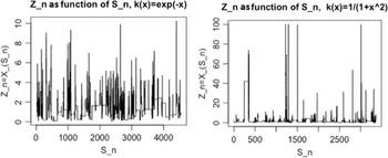
The above graphs give the positions
 $Z_n$
as a function of the jump times
 $S_n$
. The waiting times between successive jumps are longer in the first process than in the second one. Since we use the same jump rate function in both processes and since this rate is an increasing function of the positions, this is due to the fact that jumps lead to higher values in the second process than in the first, so that jumps occur more frequently.

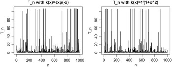
These graphs represent the sequence
 $T_{n}=S_{n}-S_{n-1} $
of the inter-jump waiting times for the two processes, showing once more that these waiting times are indeed longer in the first process than in the second.

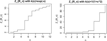
The above graphs represent the records of the two processes as a function of the ranks of the records, the one on the left with
 $k(x) = e^{-x}$
and the one on the right with
 $k(x) = 1/(1+x^2)$
. We can notice that there are more records in the first graph than in the second. Records occur more frequently in the first graph than in the second. On the other hand, the heights of the records are much lower in the first graph than in the second.

The above graphs give
 $Z_{R_n} $
as a function of
 $R_n$
. We remark that the gap between two consecutive records decreases over time, whereas the time between two consecutive records becomes longer. In other words, the higher a record is, the longer it takes to surpass it statistically.

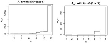
The above graphs give
 $A_n= R_n-R_{n-1} $
as a function of
 $n$
. The differences between two consecutive records are much greater in the first graph than in the second. It is also noted that the maximum time gap is reached between the penultimate record and the last record.

The above graphs give the records obtained from the simulation of the two processes, as a function of time. We remark that the curve is slowly increasing with the time. In fact, to reach the 12th record, the first simulated process needs 5500 units of time, and analogously, the second simulated process needs 1500 units of time to reach its 8th record.

6. The extremal record chain
Of interest are the upper record times and values sequences of
 $Z_{n}$
, namely
 \begin{align*}R_{n} & = \inf \!\left( r\geq 1\,:\,r>R_{n-1},Z_{r}>Z_{R_{n-1}}\right), \\Z_{n}^{*} & = Z_{R_{n}}.\end{align*}
Unless X (and so
 $Z_{n}$
) goes extinct,
 $Z_{n}^{*}$
is a strictly increasing sequence tending to
 $\infty $
.
Following [Reference Adke1], with
 $\left( R_{0}=0,Z_{0}^{*}=x\right) $
,
 $\left(R_{n},Z_{n}^{*}\right) _{n\geq 0}$
clearly is a Markov chain with transition probabilities for
 $y>x$
given by
 \begin{align*}\overline{P}^{*}\left( k,x,y\right) &\,:\!=\, \mathbb{P}\!\left(R_{n}=r+k,Z_{n}^{*}>y\mid R_{n-1}=r,Z_{n-1}^{*}=x\right) \\& \,= \overline{P}\!\left( x,y\right) \quad \text{ if }k=1 \\& \,= \int_{0}^{x}...\int_{0}^{x}\prod_{l=0}^{k-2}P\!\left( x_{l},dx_{l+1}\right)\overline{P}\!\left( x_{k-1},y\right) \quad \text{ if }k\geq 2,\end{align*}
where
 $P\!\left( x,dy\right) =\mathbb{P}\!\left( Z_{n}\in dy\mid Z_{n-1}=x\right)$
,
 $\overline{P}\!\left( x,y\right) =\mathbb{P}\!\left(Z_{n}>y\mid Z_{n-1}=x\right)$
, and
 $x_{0}=x$
.
Clearly the marginal sequence
 $\left( Z_{n}^{*}\right) _{n\geq 0}$
is Markov with transition matrix
 \begin{equation*}\overline{P}^{*}\left( x,y\right) \,:\!=\,\mathbb{P}\!\left( Z_{n}^{*}>y\mid Z_{n-1}^{*}=x\right) =\sum_{k\geq 1}\overline{P}^{*}(k,x,y),\end{equation*}
but the marginal sequence
 $\left( R_{n}\right) _{n\geq 0}$
of record times is non-Markov. However,
 \begin{equation*}\mathbb{P}\!\left( R_{n}=r+k\mid R_{n-1}=r,Z_{n-1}^{*}=x\right) =\overline{P}^{*}\left( k,x,x\right) ,\end{equation*}
showing that the law of
 $A_{n}\,:\!=\,R_{n}-R_{n-1}$
(the age of the nth record) is independent of
 $R_{n-1}$
(although not of
 $Z_{n-1}^{*}$
)
 $:$
 \begin{equation*}\mathbb{P}\!\left( A_{n}=k\mid Z_{n-1}^{*}=x\right) =\overline{P}^{*}\left(k,x,x\right), \qquad k\geq 1.\end{equation*}
Of particular interest is
 $\left( R_{1},Z_{1}^{*}=Z_{R_{1}}\right) $
, the first upper record time and value, because
 $S_{R_{1}}$
is the first time
 $(X_t)_t $
exceeds the threshold x, and
 $Z_{R_{1}}$
is the corresponding overshoot at
 $y>x$
. Its joint distribution is simply (
 $y>x$
)
 \begin{align*}P^{*}\left( k,x,dy\right) & =\mathbb{P}\!\left( R_{1}=k,Z_{1}^{*}\in dy\mid R_{0}=0,Z_{0}^{*}=x\right)\nonumber\\& = P\!\left( x,dy\right) \text{ if }k=1 \\& = \int_{0}^{x}...\int_{0}^{x}\prod_{l=0}^{k-2}P\!\left( x_{l},dx_{l+1}\right)P\!\left( x_{k-1},dy\right) \quad \text{ if }k\geq 2 .\end{align*}
If
 $y_{c}>x$
is a critical threshold above which one wishes to evaluate the joint probability of
 $\left( R_{1},Z_{1}^{*}=Z_{R_{1}}\right) $
, then
 $P^{*}\left( k,x,dy\right) /\overline{P}^{*}\left( k,x,y_{c}\right) $
for
 $y>y_{c}$
is its right expression.
Note that
 $\mathbb{P}\!\left( R_{1}=k\mid R_{0}=0,Z_{0}^{*}=x\right) =\overline{P}^{*}\left( k,x,x\right) $
and also that
 \begin{equation*}P^{*}\left( x,dy\right) \,:\!=\,\mathbb{P}\!\left(Z_{1}^{*}\in dy\mid Z_{0}^{*}=x\right) =\sum_{k\geq 1}P^{*}\left(k,x,dy\right) .\end{equation*}
Of interest also is the number of records in the set
 $\left\{0,...,N\right\} :$
 \begin{equation*}\mathcal{R}_{N}\,:\!=\,\#\left\{ n\geq 0\,:\,R_{n}\leq N\right\} =\sum_{n\geq 0}\mathbf{1}_{\left\{ R_{n}\leq N\right\} } .\end{equation*}
7. Decay–surge processes and their relationship to Hawkes and shot-noise processes
7.1. Hawkes processes
In the section we study the particular case
 $\beta \!\left(x\right) =\beta _{1}x$
,
 $\beta _{1}>0$
(the surge rate increases linearly with x),
 $\alpha(x) =\alpha _{1}x$
,
 $\alpha _{1}>0$
(exponentially declining population), and
 $k(y) =e^{-y}$
. In this case, with
 $\gamma _{1}=\beta _{1}/\alpha _{1}$
,
 $\Gamma (x)=\gamma _{1}x$
.
In this case, we remark that
 $\Gamma (0)=0>-\infty$
. Therefore there is a strictly positive probability that the process will never jump (in which case it is attracted to 0). However, we have
 $t_{0}(x)=\infty$
, so the process never hits 0 in finite time. Finally,
 $\beta (0)=0$
implies that state 0 is natural (absorbing and inaccessible).
Note that for this model,
 \begin{equation*}\pi(y) =\frac{1}{\alpha _{1}y}e^{\left( \gamma _{1}-1\right) y}\end{equation*}
and we may take a version of the scale function given by
 \begin{equation*}s (x) =\frac{\gamma _{1}}{1-\gamma _{1}}[e^{-\left( \gamma _{1}-1\right) y}]_{0}^{x } = \frac{\gamma _{1}}{1-\gamma _{1}} \left( e^{\left( 1 - \gamma _{1} \right) x}- 1 \right) .\end{equation*}
Clearly, Assumption 2 is satisfied if and only if
 $\gamma _{1}< 1$
. We call the case
 $ \gamma_1 < 1 $
subcritical, the case
 $ \gamma_1 > 1 $
supercritical, and the case
 $ \gamma_1 = 1 $
critical.
Supercritical case. It can be shown that the process does not explode almost surely, so that it is transient in this case (see Proposition 5). The speed density is integrable neither at 0 nor at
 $\infty $
.
Critical and subcritical case. If
 $\gamma_1 < 1$
, then
 $\pi $
is integrable at
 $+\infty $
, and we find
 \begin{equation*}\phi _{a}(x) =-\left[ s(y) \overline{\pi }\left( y\right) \right] _{a}^{x}-\int_{a}^{x}s(y) \pi(y) dy+\frac{1}{\alpha _{1}}\log \frac{x}{a},\end{equation*}
where (with Ei the exponential integral function)
 \begin{equation*}\int_{a}^{x}s(y) \pi(y) dy=\frac{\gamma _{1}}{\alpha _{1}\!\left( 1 - \gamma _{1} \right) }\left[ \ln \!\left( \frac{x}{a} \right) - \text{Ei}\!\left( \left( \gamma_{1}-1\right) x\right) + \text{Ei}\!\left( \left( \gamma _{1} -1\right) a\right) \right] .\end{equation*}
In the critical case
 $\gamma_1 = 1 $
, the hitting time of a will be finite without having finite expectation.
In both the critical and subcritical cases, that is, when
 $\gamma _{1}\leq 1$
, the process
 $X_t $
converges to 0 as
 $t \to \infty $
, as we shall show now.
Owing to the additive structure of the underlying deterministic flow and the exponential jump kernel, we have the explicit representation
 \begin{equation} X_t = e^{ - \alpha_1 t } x + \sum_{ n \geq 1 \,:\, S_n \le t } e^{ - \alpha_1(t- S_n ) } Y_n,\end{equation}
where the
 $(Y_n)_{n \geq 1 } $
are independent and identically distributed exponential random variables with mean 1, such that for all n,
 $Y_n $
is independent of
 $S_k$
,
 $k \le n $
, and of
 $Y_k$
,
 $k < n$
. Finally, in (25), the process
 $X_t$
jumps at rate
 $\beta_1 X_{t- }$
.
The above system is a linear Hawkes process without immigration, with kernel function
 $h( t) = e^{ - \alpha_1 t } $
and with random jump heights
 $(Y_n)_{n \geq 1 } $
(see [Reference Hawkes22]; see also [Reference Brémaud and Massoulié5]). Such a Hawkes process can be interpreted as an inhomogeneous Poisson process with branching. Indeed, the additive structure in (25) suggests the following construction:
At time 0, we start with a Poisson process having time-dependent rate
$\beta _{1}e^{-\alpha _{1}t}x$
.At each jump time S of this process, a new (time-inhomogeneous) Poisson process is born and added to the existing one. This new process has intensity
$\beta _{1}e^{-\alpha _{1}(t-S)}Y$
, where Y is exponentially distributed with parameter 1, independent of what has happened before. We call the jumps of this newborn Poisson process jumps of generation
$1$
.At each jump time of generation 1, another time-inhomogeneous Poisson process is born, of the same type, independently of anything else that has happened before. This gives rise to jumps of generation
$2$
.The above procedure is iterated until it eventually stops, since the remaining Poisson processes do not jump any more.


The total number of jumps of any of the offspring Poisson processes is given by
 \begin{equation*}\beta_1 \mathbb{E } (Y) \int_{S}^\infty e^{ - \alpha_1 (t- S ) } dt =\gamma_1.\end{equation*}
So we see that whenever
 $\gamma_1 \le 1 $
, we are considering a subcritical or critical Galton–Watson process which goes extinct almost surely, after a finite number of reproduction events. This extinction event is equivalent to the fact that the total number of jumps in the system is finite almost surely, so that after the last jump,
 $X_t$
just converges to 0 (without, however, ever reaching it). Notice that in the subcritical case
 $\gamma_1 < 1$
, the speed density is integrable at
 $ \infty$
, while it is not at 0, corresponding to absorption in
 $0$
.
An interesting feature of this model is that it can exhibit a phase transition when
 $\gamma _{1}$
crosses the value 1.
Finally, in the case of a linear Hawkes process with immigration we have
 $\beta ( x) = \mu + \beta_1 x $
, with
 $\mu > 0$
. In this case,
 \begin{equation*}\pi( y) =\frac{1}{\alpha _{1}}e^{\left( \gamma _{1}-1\right) y } y^{ \mu/\alpha_1 - 1 },\end{equation*}
which is always integrable in 0 and which can be tuned into a probability in the subcritical case
 $\gamma_1 < 1$
corresponding to positive recurrence.
Remark 15. An interpretation of the decay–surge process in terms of Hawkes processes is only possible in the case of affine jump rate functions
 $ \beta$
, additive drift
 $ \alpha $
, and exponential kernels k as considered above.
7.2. Shot-noise processes
Let
 $h\!\left( t\right) $
,
 $t\geq 0$
, with
 $h\!\left( 0\right) =1$
be a causal non-negative non-increasing response function translating the way shocks will attenuate as time passes in a shot-noise process. We assume
 $h\!\left(t\right) \rightarrow 0$
as
 $t\rightarrow \infty $
and
 \begin{equation}\int_{0}^{\infty }h\!\left( s\right) ds<\infty . \end{equation}
With
 $X_{0}=x\geq 0$
, consider then the linear shot-noise process
 \begin{equation}X_{t}=x+\int_{0}^{t}\int_{{\Bbb R}_{+}}yh\!\left( t-s\right) \mu \!\left(ds,dy\right) , \end{equation}
where, with
 $\left( S_{n};\,n\geq 1\right) $
being the points of a homogeneous Poisson point process with intensity
 $\beta$
,
 $\mu \!\left( ds,dy\right)=\sum_{n\geq 1}\delta _{S_{n}}\left( ds\right) \delta _{\Delta _{n}}\left(dy\right) $
(translating to independence of the shot heights
 $\Delta _{n}$
and occurrence times
 $S_{n}$
). Note that, with
 $dN_{s}=\sum_{n\geq1}\Delta _{n}\delta _{S_{n}}\left( ds\right)$
, so with
 $N_{t}=\sum_{n\geq1}\Delta _{n}{\bf 1}_{\{ S_{n}\leq t \}} $
representing a time-homogeneous compound Poisson process with jump amplitudes
 $\Delta$
,
 \begin{equation}X_{t}=x+\int_{0}^{t}h\!\left( t-s\right) dN_{s} \end{equation}
is a linearly filtered compound Poisson process. In this form, it is clear that
 $X_{t}$
cannot be Markov unless
 $h\!\left( t\right) =e^{-\alpha t}$
,
 $\alpha >0$
. We define
 \begin{align*}\nu \!\left( dt,dy\right) & = {\mathbb{ P}}\!\left( S_{n}\in dt,\Delta _{n}\in dy\text{for some }n\geq 1\right) \\& = \beta dt\cdot {\mathbb{ P}}\!\left( \Delta \in dy\right) .\end{align*}
In the sequel, we shall assume without much loss of generality that
 $x=0$
.
The linear shot-noise process
 $X_{t}$
has two alternative equivalent representations, emphasizing its superposition characteristics:
 \begin{align*}\left( 1\right) \text{ }X_{t} & = \sum_{n\geq 1}\Delta _{n}h\!\left(t-S_{n}\right) {\bf 1}_{\{ S_{n}\leq t\}}, \\\left( 2\right) \text{ }X_{t} & = \sum_{p=1}^{P_{t}}\Delta _{p}h( t-{\mathcal{S}}_{p}(t)),\end{align*}
where
 $P_t = \sum_{n\geq1} {\bf 1}_{\{ S_{n}\leq t\}}$
.
Both show that
 $X_{t}$
is the size at t of the whole decay–surge population, summing up all the declining contributions of the sub-families which appeared in the past at jump times (a shot-noise or filtered Poisson process model appearing also in physics and queuing theory; see [Reference Snyder and Miller32] and [Reference Parzen28]). The contributions
 $\Delta _{p}h\!\left( t-{\mathcal{S}}_{p}\left(t\right) \right) $
,
 $p=1, ...P_{t}$
, of the
 $P_{t}$
families to
 $X_{t}$
are stochastically ordered in decreasing sizes.
In the Markov case,
 $h\!\left( t\right) =e^{-\alpha t}$
,
 $t\geq 0$
,
 $\alpha >0$
, we have
 \begin{equation}X_{t}=e^{-\alpha t}\int_{0}^{t}e^{\alpha s}dN_{s}, \end{equation}
so that
 \begin{equation*}dX_{t}=-\alpha X_{t}dt+dN_{t},\end{equation*}
showing that
 $X_{t}$
is a time-homogeneous Markov process driven by
 $N_{t}$
, known as the classical linear shot-noise. This is clearly the only choice of the response function that makes
 $X_{t}$
Markov. In that case, by Campbell’s formula (see [Reference Parzen28]),
 \begin{align*}\Phi _{t}^{X}\!\left( q\right) &\,:\!=\, {\mathbb{ E}}e^{-qX_{t}}=e^{-\beta\int_{0}^{t}\left( 1-\phi _{\Delta }\left( qe^{-\alpha \!\left( t-s\right)}\right) \right) ds} \\& = e^{-\frac{\beta }{\alpha }\int_{e^{-\alpha t}}^{1}\frac{1-\phi _{\Delta}\left( qu\right) }{u}du} \quad \text{ where }e^{-\alpha s}=u,\end{align*}
with
 \begin{equation*}\Phi _{t}^{X}\left( q\right) \rightarrow \Phi _{\infty }^{X}\left( q\right)=e^{-\frac{\beta }{\alpha }\int_{0}^{1}\frac{1-\phi _{\Delta }\left(qu\right) }{u}du} \quad \text{ as }t\rightarrow \infty .\end{equation*}
The simplest explicit case is when
 $\phi _{\Delta }\left( q\right) =1/\left(1+q/\theta \right) $
(otherwise
 $\Delta \sim $
Exp
 $\left( \theta \right) $
), so that, with
 $\gamma =\beta /\alpha$
,
 \begin{equation*}\Phi _{\infty }^{X}\left( q\right) =\left( 1+q/\theta \right) ^{-\gamma },\end{equation*}
the Laplace–Stieltjes transform of a Gamma
 $\left( \gamma ,\theta \right) $
-distributed random variable
 $X_{\infty }$
, with density
 \begin{equation*}\frac{\theta ^{\gamma }}{\Gamma \!\left( \gamma \right) }x^{\gamma-1}e^{-\theta x}\text{, } \qquad x>0.\end{equation*}
This time-homogeneous linear shot-noise process with exponential attenuation function and exponentially distributed jumps is a decay–surge Markov process with triple
 \begin{equation*}\left( \alpha(x) =-\alpha x;\text{ }\beta (x)=\beta ;\text{ }k(x) =e^{-\theta x}\right) .\end{equation*}
Shot-noise processes being generically non-Markov, there is no systematic relationship between decay–surge Markov processes and shot-noise processes. In [Reference Eliazar and Klafter14], it is pointed out that decay–surge Markov processes could be related to the maximal process of nonlinear shot noise; see Eliazar and Klafter [Reference Eliazar and Klafter13, Reference Eliazar and Klafter14].
Funding information
T. Huillet acknowledges partial support from the Chaire Modélisation mathématique et biodiversité. B. Goncalves and T. Huillet acknowledge support from the Labex MME-DII Center of Excellence (Modèles mathématiques et économiques de la dynamique, de l’incertitude et des interactions, project ANR-11-LABX-0023-01). This work was funded by the CY Initiative of Excellence (grant Investissements d’Avenir, ANR-16-IDEX-0008), project EcoDep PSI-AAP2020-0000000013.
Competing interests
There were no competing interests to declare which arose during the preparation or publication process for this article.