1 Introduction
Detonation formation processes are usually classified as either direct initiation or deflagration-to-detonation transition (DDT). Direct initiation (Eckett, Quirk & Shepherd Reference Eckett, Quirk and Shepherd2000) uses a relatively large amount of energy deposited in a short time period (classically, instantaneous energy deposition to a point) to create a significant thermomechanical response in the gas leading to a blast wave within the reactive mixture. A typical DDT process begins by igniting the gas using a comparatively small amount of energy to create a laminar flame. Surface instabilities at the flame front (Oppenheim et al. Reference Oppenheim, Kuhl, Lundstrom and Kamel1972; Roy et al. Reference Roy, Frolov, Borisov and Netzer2004; Oran & Gamezo Reference Oran and Gamezo2007) transform the deflagration to a turbulent reaction front, which enhances the rate of thermal energy conversion. Compression waves are produced by a transient thermomechanical response arising from the enhanced rate of energy release from the increase in reaction front surface area. Compression waves propagate ahead of the evolving reaction zone, precondition the reactive gas ahead of the reaction front and coalesce until a detonation wave is formed. Oppenheim & Soloukhin (Reference Oppenheim and Soloukhin1973) address these concepts with the prescient remark that ‘Gasdynamics of explosions is best defined as the science dealing with the interrelationship between energy transfer occurring at a high rate in a compressible medium and the concomitant motion set up in this medium’. In the years since their paper was published, modellers have endeavoured to quantify the cited interrelationship, including the impact of viscous/diffusive transport effects (Powers Reference Powers2006; Oran & Gamezo Reference Oran and Gamezo2007; Radulescu et al. Reference Radulescu, Sharpe, Law and Lee2007; Dorofeev Reference Dorofeev2011; Mazaheri, Mahmoudi & Radulescu Reference Mazaheri, Mahmoudi and Radulescu2012; Romick, Aslam & Powers Reference Romick, Aslam and Powers2012).
Direct initiation and DDT can be characterized by using concepts in the thermomechanical analyses by Kassoy (Reference Kassoy2010, Reference Kassoy2014a
, Reference Kassoy2016). The first describes the consequences of localized, transient, spatially distributed thermal power deposition from a source into a volume (characteristic length-scale
 $l$
) of inert gas on a time scale,
 $t_{h}$
, that is short compared to the characteristic acoustic time,
 $t_{a}=l/a$
, where
 $a$
is the characteristic acoustic velocity of the heated volume. The thermomechanical response of the gas can be characterized as nearly constant volume heating when the energy addition is less than an explicitly defined maximum value. Pressure rises with temperature, leading to a pressure gradient that can accelerate fluid particles. The result is a low-Mach-number internal expansion process. Gas expelled from the original hot spot volume acts like a piston driving mechanical disturbances into the neighbouring unheated gas. The amount of energy added to the volume determines the amplitude of the mechanical disturbances (e.g, acoustic, shock, or blast waves). The maximum energy addition leads to a fully compressible expansion process characterized by an
 $O(1)$
Mach number and the generation of very strong shocks. In contrast, when the heating time is much longer than the characteristic acoustic time,
 $t_{h}\gg t_{a}$
, the heat addition process occurs at a nearly spatially homogeneous pressure, with density declining inversely with temperature increase.
A detonation can be initiated by localized, transient, spatially distributed thermal power deposition on a time scale similar to the acoustic time scale of the heated fluid volume. Previous work in this area describes 1-D solutions of the reactive Euler equations (Clarke, Kassoy & Riley Reference Clarke, Kassoy and Riley1986; Clarke et al. Reference Clarke, Kassoy, Meharzi, Riley and Vasantha1990; Sileem, Kassoy & Hayashi Reference Sileem, Kassoy and Hayashi1991; Kassoy et al. Reference Kassoy, Kuehn, Nabity and Clarke2008; Regele, Kassoy & Vasilyev Reference Regele, Kassoy and Vasilyev2012). The reactive mixture is initially at rest. Spatially resolved thermal power deposition occurs in a finite subvolume of the fluid. Shock waves are created by the initial power deposition. In the earliest work, energy is added by conduction from a planar wall located at one end of the reactive gas domain (Clarke et al. Reference Clarke, Kassoy and Riley1986, Reference Clarke, Kassoy, Meharzi, Riley and Vasantha1990). Alternatively, heat is added directly to a specified fluid volume (Sileem et al. Reference Sileem, Kassoy and Hayashi1991; Kassoy et al. Reference Kassoy, Kuehn, Nabity and Clarke2008). Typically, an isolated high-temperature hot spot evolves spontaneously on a time scale that is short compared to the local characteristic acoustic time scale in response to exothermic reaction initiation. A detonation follows. These 1-D studies are carried out for relatively low activation energies. Recently, the work was extended to higher activation energies (Regele et al. Reference Regele, Kassoy and Vasilyev2012). Multiple isolated high-temperature hot spots characterize the combustion process in relatively high activation energy mixtures.
Kurtz & Regele (Reference Kurtz and Regele2014a
,Reference Kurtz and Regele
b
) perform numerical simulations of isolated hot spots in one and two dimensions. The hot spots are modelled as a linear temperature gradient adjacent to a constant temperature plateau of some prescribed size in order to account for the finite size of localized hot spot maxima. Hot spots are shown to produce acoustic waves, compression waves and shock waves. They demonstrate that the predicted behaviour can be characterized by examining the ratio of the heating to acoustic time scale ratio
 $t_{h}/t_{a}$
.
Hot spots can form inside a turbulent flame brush and initiate a rapid reaction process (explosion) to create a detonation wave (Khokhlov & Oran Reference Khokhlov and Oran1999). Obstacles inside a channel, such as a Schelkin spiral, can increase flow turbulence and reaction zone surface area/volume. The concomitant increase in rate of heat release leads to compression waves that precondition the gas and form a detonation wave (Gamezo, Ogawa & Oran Reference Gamezo, Ogawa and Oran2008). It has also been shown that boundary layers can be the sites of localized explosions that facilitate detonation formation (Ivanov, Kiverin & Liberman Reference Ivanov, Kiverin and Liberman2011). The Navier–Stokes (NS) equations are normally employed when performing numerical simulations of DDT (Khokhlov & Oran Reference Khokhlov and Oran1999; Khokhlov, Oran & Thomas Reference Khokhlov, Oran and Thomas1999; Oran & Khokhlov Reference Oran and Khokhlov1999; Gamezo, Khokhlov & Oran Reference Gamezo, Khokhlov and Oran2001; Oran & Gamezo Reference Oran and Gamezo2007; Kessler, Gamezo & Oran Reference Kessler, Gamezo and Oran2010; Ivanov et al.
Reference Ivanov, Kiverin and Liberman2011). In the instances where the Euler equations are solved without the diffusive/viscous terms, the numerical diffusion implicitly present in the hyperbolic solver is used to mimic the effects of molecular viscosity/diffusion (Gamezo, Desbordes & Oran Reference Gamezo, Desbordes and Oran1999). In the context of detonation evolution many investigators have assessed the impact of viscous/diffusive transport effects (Gamezo et al.
Reference Gamezo, Khokhlov and Oran2001; Radulescu et al.
Reference Radulescu, Sharpe, Lee, Kiyanda, Higgins and Hanson2005; Powers Reference Powers2006; Radulescu et al.
Reference Radulescu, Sharpe, Law and Lee2007; Romick et al.
Reference Romick, Aslam and Powers2012; Mazaheri et al.
Reference Mazaheri, Mahmoudi and Radulescu2012) and found some small-scale difference when compared to the results of fully resolved NS simulations (Powers Reference Powers2006). Kassoy (Reference Kassoy2010, Reference Kassoy2014b
) has used non-dimensionalized inert and reactive NS equations to identify parameters that modulate viscous, conduction, diffusion and dissipation terms in order to determine when Euler equation models may be valid. The results show that all non-dimensional transport terms (differential operators) are modulated by the product of two parameters, either one of which can be asymptotically small: the inverse acoustic Reynolds number (Knudsen number) and the ratio of the heating time scale to the local acoustic time scale. Even if the latter is
 $O(1)$
, as in the current modelling, a typical value for the Knudsen number,
 $10^{-7}$
, implies that local non-dimensional transport gradients must be enormous in order for viscous diffusion, conduction dissipation and mass diffusion to be of importance in the physics of the processes.
Sileem et al. (Reference Sileem, Kassoy and Hayashi1991), Kassoy et al. (Reference Kassoy, Kuehn, Nabity and Clarke2008) and Regele et al. (Reference Regele, Kassoy and Vasilyev2012) have modelled one-dimensional (1-D), acoustic time-scale detonation initiation using the Euler equations. The 1-D acoustic time scale detonation initiation results show that it is possible to initiate a planar detonation wave with physically plausible properties. The current objective is to extend the 1-D acoustic time scale approach (
 $t_{h}=O(t_{a})$
) to planar two-dimensional (2-D) Euler and NS-based models in order to describe the physics of detonation initiation. In order to maintain consistency with the previous 1-D model (Regele et al.
Reference Regele, Kassoy and Vasilyev2012), a solution is pursued that is independent of diffusive/viscous transport effects. In that context, the evolution arises from the purely reactive gasdynamics envisioned by Oppenheim & Soloukhin (Reference Oppenheim and Soloukhin1973).
Consideration of multiple dimensions allows effects such as the Richtmyer–Meshkov and Kelvin–Helmholtz instabilities to exist. The Richtmyer–Meshkov instability is found to be the primary source of turbulence generation in DDT (Oran & Gamezo Reference Oran and Gamezo2007; Gamezo et al. Reference Gamezo, Khokhlov and Oran2001). Kelvin–Helmholtz instabilities can also be found in DDT as a secondary instability and are often suppressed by diffusive effects in NS solutions (Oran & Gamezo Reference Oran and Gamezo2007). In order to obtain a purely gasdynamic detonation initiation solution, it will be necessary to capture both the Richtmyer–Meshkov and Kelvin–Helmholtz instabilities. It will also be necessary to minimize the numerical diffusion such that any unreacted pockets will have a minimal amount of heat diffused into them so that their autoignition times can be resolved.
A moderately low activation energy will be used that is similar to that of the mildly unstable detonation case in Radulescu et al. (Reference Radulescu, Sharpe, Law and Lee2007) and Radulescu & Maxwell (Reference Radulescu and Maxwell2011). The approach taken in this work is to quantitatively justify the use of the Euler equation model and solve them with increasing levels of resolution until the detonation formation time and the spatially integrated chemical heat release transient are no longer affected by the unresolved local flow structures. In this paper a series of numerical experiments with progressively increasing resolution is conducted in order to quantitatively demonstrate that acoustic time-scale detonation initiation is dominated by purely gasdynamic effects and is independent of diffusive/viscous transport effects. These Euler simulations are cross-referenced against solutions of the NS equations with sufficiently large Reynolds numbers to demonstrate the validity of the approach.
2 Mathematical model
The mathematical model for quantifying the thermomechanical response of a compressible, reactive gas to localized, spatially distributed power deposition from an external source and ultimately from a one-step Arrhenius-type chemical reaction is based on the vector form of the non-dimensional reactive NS equations
 $$\begin{eqnarray}\displaystyle & \displaystyle \unicode[STIX]{x1D70C}_{t}+\unicode[STIX]{x1D735}\boldsymbol{\cdot }\unicode[STIX]{x1D70C}\boldsymbol{u}=0, & \displaystyle\end{eqnarray}$$
 $$\begin{eqnarray}\displaystyle & \displaystyle (\unicode[STIX]{x1D70C}\boldsymbol{u})_{t}+\unicode[STIX]{x1D735}\boldsymbol{\cdot }(\unicode[STIX]{x1D70C}\boldsymbol{u}\boldsymbol{u})=-\unicode[STIX]{x1D735}P+\frac{1}{Re_{a}}\unicode[STIX]{x1D735}\boldsymbol{\cdot }\unicode[STIX]{x1D749} & \displaystyle\end{eqnarray}$$
 $$\begin{eqnarray}\displaystyle & \displaystyle (\unicode[STIX]{x1D70C}e_{T})_{t}+\unicode[STIX]{x1D735}\boldsymbol{\cdot }(\boldsymbol{u}(\unicode[STIX]{x1D70C}e_{T}+P))=\dot{Q}(\boldsymbol{x},t)+{\dot{W}}q+\frac{1}{Re_{a}Pr}\unicode[STIX]{x1D735}\boldsymbol{\cdot }(\unicode[STIX]{x1D735}T)+\frac{1}{Re_{a}}\unicode[STIX]{x1D735}\boldsymbol{\cdot }(\boldsymbol{u}\boldsymbol{\cdot }\unicode[STIX]{x1D749})\qquad & \displaystyle\end{eqnarray}$$
 $$\begin{eqnarray}\displaystyle & \displaystyle (\unicode[STIX]{x1D70C}Y)_{t}+\unicode[STIX]{x1D735}\boldsymbol{\cdot }\unicode[STIX]{x1D70C}Y\boldsymbol{u}=-{\dot{W}}+\frac{1}{Re_{a}Sc}\unicode[STIX]{x1D735}\boldsymbol{\cdot }(\unicode[STIX]{x1D70C}\unicode[STIX]{x1D735}Y). & \displaystyle\end{eqnarray}$$
Here the stress tensor is
 $\unicode[STIX]{x1D749}=-(2/3)(\unicode[STIX]{x1D735}\boldsymbol{\cdot }\boldsymbol{u})\unicode[STIX]{x1D644}+\unicode[STIX]{x1D735}\boldsymbol{u}+\unicode[STIX]{x1D735}\boldsymbol{u}^{\text{T}}$
, where
 $\unicode[STIX]{x1D644}$
is the identity matrix. These equations are complimented by an equation of state written in terms of
 $e_{T}$
and
 $\boldsymbol{u}$
 $$\begin{eqnarray}P=(\unicode[STIX]{x1D6FE}-1)\unicode[STIX]{x1D70C}\left(e_{T}-\frac{\boldsymbol{u}\boldsymbol{\cdot }\boldsymbol{u}}{2}\right).\end{eqnarray}$$
Finally the reaction rate is defined by
 $$\begin{eqnarray}{\dot{W}}=B\unicode[STIX]{x1D70C}Ye^{-E/T},\end{eqnarray}$$
where the temperature is expressed as
 $T=\unicode[STIX]{x1D6FE}P/\unicode[STIX]{x1D70C}$
and
 $\dot{Q}(\boldsymbol{x},t)$
is the non-dimensional thermal power deposition term.
The non-dimensional thermodynamic variables are defined by
 $$\begin{eqnarray}(\unicode[STIX]{x1D70C},P,T)=\left(\frac{\unicode[STIX]{x1D70C}^{\prime }}{\unicode[STIX]{x1D70C}_{0}^{\prime }},\frac{p^{\prime }}{\unicode[STIX]{x1D6FE}p_{0}^{\prime }},\frac{T^{\prime }}{T_{0}^{\prime }}\right),\end{eqnarray}$$
where primes denote dimensional variables and
 $(\unicode[STIX]{x1D70C}_{0}^{\prime },p_{0}^{\prime },T_{0}^{\prime })$
are the reference (initial) values of the density, pressure and temperature. The non-dimensional velocity is defined by
 $$\begin{eqnarray}\boldsymbol{u}=\frac{\boldsymbol{u}^{\prime }}{a_{0}^{\prime }},\end{eqnarray}$$
where
 $a_{0}^{\prime }$
is the acoustic speed in the reference state. The space and time variables are defined by
 $$\begin{eqnarray}\boldsymbol{x}=\frac{\boldsymbol{x}^{\prime }}{l^{\prime }},\quad t=\frac{t^{\prime }}{t_{a}^{\prime }},\end{eqnarray}$$
where
 $l^{\prime }$
is the characteristic length-scale of the volume affected initially by the external non-dimensional power source
 $\dot{Q}=\dot{Q}^{\prime }/{a^{\prime }}_{0}^{2}$
, defined with respect to the dimensional power source
 $\dot{Q}^{\prime }$
and the square of the sound speed in the reference state. The source is assumed to have a characteristic power addition time scale denoted by
 $t_{e}^{\prime }$
. The acoustic time scale, defined by
 $t_{a}^{\prime }=l^{\prime }/a_{0}^{\prime }$
, represents the characteristic time for an acoustic disturbance to propagate across the volume. Kassoy (Reference Kassoy2010, Reference Kassoy2014a
,Reference Kassoy
b
, Reference Kassoy2016) has demonstrated the significance of the relative magnitudes of
 $t_{e}^{\prime }$
and
 $t_{a}^{\prime }$
when quantifying thermomechanical responses of gases to thermal energy deposition. The ratio of specific heats,
 $\unicode[STIX]{x1D6FE}$
, has the usual definition, the non-dimensional pre-exponential factor,
 $B=B^{\prime }t_{a}^{\prime }$
, is defined with respect to the dimensional pre-exponential factor
 $B^{\prime }$
and the acoustic time scale. The non-dimensional heat of reaction,
 $q=q^{\prime }/{a^{\prime }}_{0}^{2}$
, is defined with respect to the dimensional heat of reaction
 $q^{\prime }$
and the square of the sound speed in the reference state. The non-dimensional activation energy number is defined in familiar terms,
 $E=E^{\prime }/R^{\prime }T_{0}^{\prime }$
. The critical parameter in (2.1) is the acoustic Reynolds number (the inverse of the Knudsen number) defined by
 $Re_{a}=a_{0}^{\prime }l^{\prime }/\unicode[STIX]{x1D708}_{0}^{\prime },$
where
 $\unicode[STIX]{x1D708}_{0}^{\prime }$
is the kinematic viscosity at temperature
 $T_{0}^{\prime }$
. Other familiar parameters are the Prandtl and Schmidt numbers
 $Pr$
and
 $Sc$
, respectively.
The inverse of the acoustic Reynolds number modulates each and every transport term in (2.1). In this respect it is important to understand the magnitude of that term for a range of typical values of the volume dimension,
 $l^{\prime }$
, and the reference state. For example, a gas with a speed of sound
 $a_{0}^{\prime }=350~\text{m}~\text{s}^{-1}$
, kinematic viscosity
 $\unicode[STIX]{x1D708}^{\prime }=10^{-6}~\text{m}^{2}~\text{s}^{-1}$
and characteristic length
 $l^{\prime }=10^{-3}~\text{m}$
, the acoustic Reynolds number is
 $Re_{a}=O(10^{5})$
.
If the acoustic Reynolds number is sufficiently large, transport terms in (2.1) can be ignored during the external power deposition process, resulting in the reactive Euler equations
 $$\begin{eqnarray}\displaystyle & \displaystyle \unicode[STIX]{x1D70C}_{t}+\unicode[STIX]{x1D735}\boldsymbol{\cdot }\unicode[STIX]{x1D70C}\boldsymbol{u}=0, & \displaystyle\end{eqnarray}$$
 $$\begin{eqnarray}\displaystyle & \displaystyle (\unicode[STIX]{x1D70C}\boldsymbol{u})_{t}+\unicode[STIX]{x1D735}\boldsymbol{\cdot }(\unicode[STIX]{x1D70C}\boldsymbol{u}\boldsymbol{u})+\unicode[STIX]{x1D735}P=0, & \displaystyle\end{eqnarray}$$
 $$\begin{eqnarray}\displaystyle & \displaystyle (\unicode[STIX]{x1D70C}e_{T})_{t}+\unicode[STIX]{x1D735}\boldsymbol{\cdot }(\boldsymbol{u}(\unicode[STIX]{x1D70C}e_{T}+P))=\dot{Q}(\boldsymbol{x},t)+{\dot{W}}q, & \displaystyle\end{eqnarray}$$
 $$\begin{eqnarray}\displaystyle & \displaystyle (\unicode[STIX]{x1D70C}Y)_{t}+\unicode[STIX]{x1D735}\boldsymbol{\cdot }\unicode[STIX]{x1D70C}Y\boldsymbol{u}=-{\dot{W}}. & \displaystyle\end{eqnarray}$$
It should be noted that the local acoustic Reynolds number may differ from the global reference value defined in the paragraph below (2.4). For example, a local acoustic Reynolds number
 $Re_{ah}=l_{h}^{\prime }a_{h}^{\prime }\unicode[STIX]{x1D70C}_{h}^{\prime }/\unicode[STIX]{x1D707}_{h}^{\prime }$
can be defined in terms of the new length scale,
 $l_{h}^{\prime }$
, representing a local reactive length scale, the speed of sound in a hot reactive gas,
 $a_{h}^{\prime }$
, and the relevant value of the dynamic viscosity at a high temperature,
 $\unicode[STIX]{x1D707}_{h}^{\prime }$
, where subscript ‘
 $h$
’ refers to local conditions in the reacted system. This can be simplified by dividing by the original
 $Re_{a}$
using the temperature relation
 $\unicode[STIX]{x1D6FE}P=\unicode[STIX]{x1D70C}T$
and using a power law dynamic viscosity model. The following relation between local and global acoustic Reynolds numbers holds:
 $$\begin{eqnarray}\frac{Re_{ah}}{Re_{a}}=\frac{l_{h}^{\prime }}{l^{\prime }}\frac{\unicode[STIX]{x1D6FE}P}{T^{\unicode[STIX]{x1D714}+1/2}},\end{eqnarray}$$
where the
 $P$
and
 $T$
are non-dimensional pressure and temperature,
 $\unicode[STIX]{x1D714}$
comes from the temperature dependence of the dynamic viscosity, and the
 $1/2$
indirectly comes from the speed of sound dependence on temperature. The challenge is to estimate the magnitude of
 $l_{h}^{\prime }$
. Assuming that
 $l_{h}^{\prime }=O(l^{\prime })$
, it is plausible that the local Reynolds number substantially differs from the global one. That can be assessed from the data. The characteristic time scale for the reactive heating process can differ from the acoustic time scale
 $t_{a}$
defined in the paragraph below (2.4). The magnitude is inherent in the definition of the chemical kinetics in (2.1f
).
3 Numerical approach
Since the ultimate objective of this work is to explain how a purely gasdynamic (transport-independent) detonation initiation evolves, a multiresolution hyperbolic solver is desired. In this study the parallel adaptive wavelet-collocation method (PAWCM) is used to perform the simulations. The PAWCM is a parallel version of the original adaptive wavelet-collocation method (Vasilyev & Bowman Reference Vasilyev and Bowman2000; Kevlahan & Vasilyev Reference Kevlahan and Vasilyev2005) that incorporates Zoltan dynamic load balancing to equally distribute the computational load amongst several processors. The PAWCM combines second-generation wavelets with a prescribed error threshold parameter
 $\unicode[STIX]{x1D716}$
to determine which grid points are necessary in order to achieve a prescribed level of accuracy.
The hyperbolic solver developed for the PAWCM is used to maintain numerical stability and reduce spurious oscillations across jump discontinuities (Regele & Vasilyev Reference Regele and Vasilyev2009). As is common with many total variation diminishing hyperbolic solvers (Laney Reference Laney1998; Toro Reference Toro1999), the method is first-order accurate near shocks and contact discontinuities, and higher-order accurate in continuous regions. Other than the minimum grid spacing, the numerical diffusion/viscosity, which is implicitly present in the discontinuous regions of the flow, is the primary source of grid dependence in the present work (Regele & Vasilyev Reference Regele and Vasilyev2009; Regele et al. Reference Regele, Kassoy and Vasilyev2012). A solution is found by increasing the maximum level of resolution and thus decreasing the artificial diffusion/viscosity until the spatially integrated heat release transient is determined to be independent of grid resolution.
4 Resolution dependence in one dimension
Before performing 2-D numerical simulations of purely gasdynamic acoustic time scale detonation initiation and analysing the solution sensitivity to numerical resolution, it is helpful to assess the numerical sensitivity of a previously performed 1-D simulation (Sileem et al. Reference Sileem, Kassoy and Hayashi1991; Kassoy et al. Reference Kassoy, Kuehn, Nabity and Clarke2008; Regele et al. Reference Regele, Kassoy and Vasilyev2012). In this section, Case 1 from Regele et al. (Reference Regele, Kassoy and Vasilyev2012) is performed at multiple levels of resolution. The objective is to demonstrate that in one dimension the peak heat release time is relatively insensitive to grid spacing for a wide range of resolution.
The problem is solved using the 1-D reactive Euler equations (2.5a )–(2.5d ), the equation of state (2.1e ) and the Arrhenius reaction rate equation (2.1f ). Initially the reactive gas is at rest in thermal equilibrium with the initial condition
 $$\begin{eqnarray}\displaystyle \unicode[STIX]{x1D70C}_{o}=T_{o}=Y_{o}=1\quad u_{o}=0. & & \displaystyle\end{eqnarray}$$
A spatially resolved, transient thermal power deposition
 $$\begin{eqnarray}\displaystyle & \dot{Q}(x,t)=\left\{\begin{array}{@{}ll@{}}0 & 0\leqslant x\leqslant 1\\ 3f(t)\cos \left[\displaystyle \frac{\unicode[STIX]{x03C0}}{4}(3-x)\right] & 1<x\leqslant 5\\ 0 & x>5\end{array}\right. & \displaystyle\end{eqnarray}$$
 $$\begin{eqnarray}\displaystyle & f(t)=0.7(\tanh [5(t-t_{A})]-\tanh [5(t-t_{B})]), & \displaystyle\end{eqnarray}$$
 $x\in [1,5]$
near the adiabatic reflecting wall located at
 $x=0$
. For this simulation the heat addition is limited within the times
 $t_{A}=0.5$
and
 $t_{B}=10$
. The
 $f(t)$
profile, given by (4.3), is characterized by a fast rise to a plateau value sustained over a much longer period of time and then a fast decline near the end of the heating period. The original parameters (Regele et al.
Reference Regele, Kassoy and Vasilyev2012) use specific heat ratio
 $\unicode[STIX]{x1D6FE}=1.4$
, heat of reaction
 $q=15$
(
 $q^{\prime }/(R^{\prime }T_{0}^{\prime })=21$
), pre-exponential factor
 $B=15$
and activation energy
 $E=E^{\prime }/(R^{\prime }T_{0}^{\prime })=13.79$
. The activation energy used here is low and is of the order of activation energies typical of hydrogen–oxygen or acetylene–oxygen mixtures (Radulescu & Maxwell Reference Radulescu and Maxwell2011; Mazaheri et al.
Reference Mazaheri, Mahmoudi and Radulescu2012).
Four different simulations are performed using a base grid resolution
 $M_{x}=200$
. The effective grid resolution is specified in terms of the maximum level of resolution
 $j_{max}$
such that the effective grid resolution
 $n_{x}=M_{x}\times 2^{j_{max}}$
. Effective grid resolutions
 $n_{x}$
for the study range from 3200 to 51 200 for
 $j_{max}=4$
to
 $j_{max}=8$
.
Convergence comparisons are made using the spatially integrated chemical heat release. The global heat release transient is defined as the spatial integral over the fluid volume
 $V$
of the chemical heat release rate at an instant in time so that
 $$\begin{eqnarray}\dot{Q}_{ch}(t)=\int _{V}{\dot{W}}(\boldsymbol{x},t)q\,\text{d}V.\end{eqnarray}$$
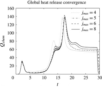
Figure 1 shows the spatially integrated heat release as a function of different levels of resolution. The first peak corresponds to the chemical reaction that occurs following the initial localized thermal power addition (4.2) and (4.3). The global maximum corresponds to the emergence of an overdriven detonation wave. A full exposition of the results can be found in Regele et al. (Reference Regele, Kassoy and Vasilyev2012).
Global heat-release curves are shown for varying levels of grid resolution. The peak heat release time varies by less than 6 % over the entire resolution range.

The results show that the peak heat release time in a 1-D acoustic time scale DDT is a weak function of numerical resolution because the smallest-scale structures contain very little reactant and are the sources of a tiny amount of energy release. At the minimum resolution
 $j_{max}=4$
, the peak heat release time is within
 $5\,\%$
of the converged value.
5 Two-dimensional detonation initiation
The 1-D model analysed in the previous section is extended to two dimensions by focusing the power deposition into a circular volume of fluid inside a rectangular domain. Simulations are performed at five different levels of resolution, where each increase in resolution effectively reduces the minimum grid spacing by one half. Section 5.2 contains a general overview of the reaction evolution and a detailed analysis of the localized reactions that govern the reaction process are given in §§ 5.3 and 5.4.
5.1 Problem statement
Each simulation begins with the reactive gas at rest with the initial condition
 $$\begin{eqnarray}\displaystyle \unicode[STIX]{x1D70C}_{0}=p_{0}=Y_{0}=1\quad \boldsymbol{v}_{0}=0, & & \displaystyle\end{eqnarray}$$
and transient thermal power deposition
 $\dot{Q}$
defined as
 $$\begin{eqnarray}\displaystyle & \dot{Q}(\boldsymbol{x},t)=8.4(\tanh [10(t-t_{A})]-\tanh [10(t-t_{B})])g(\boldsymbol{x}) & \displaystyle\end{eqnarray}$$
 $$\begin{eqnarray}\displaystyle & g(\boldsymbol{x})=\left\{\begin{array}{@{}ll@{}}1\quad & \text{for }|\boldsymbol{x}|\leqslant R\\ 0\quad & \text{for }|\boldsymbol{x}|>R.\end{array}\right. & \displaystyle\end{eqnarray}$$
 $g(\boldsymbol{x})$
limits the power addition to a circle of radius
 $R=2$
centred at the origin. The power deposition lasts from
 $t_{A}=0.5$
until
 $t_{B}=5.25$
. The time dependence in (5.2) has properties similar to those of
 $f(t)$
in (4.3). However the rise time is much shorter, approximately an interval of
 $0.3$
. Given the definition of the non-dimensional time
 $t$
, this means that the initial burst of the energy addition occurs on a short time scale compared to the local characteristic acoustic time. This kind of ‘fast’ energy addition is associated with nearly constant volume heat addition with pressure rising with temperature Kassoy (Reference Kassoy2010, Reference Kassoy2014b
). The domain lies in
 $x\in [-3,57]$
and
 $y\in [-3,9]$
and reflecting slip walls are present on all walls except the exit
 $x=57$
. The maximum level of resolution is varied from
 $5\leqslant j_{max}\leqslant 9$
with a base grid of
 $30\times 6$
. This corresponds to an effective grid of 15 360
 $\times$
3072 for the
 $j_{max}=9$
case.
5.2 General behaviour
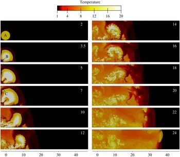
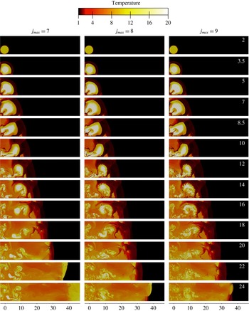
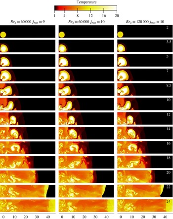
A sequence of temperature contours (figure 2) for
 $2\leqslant t\leqslant 24$
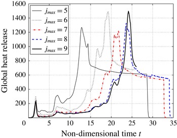
and the spatially integrated heat release at each moment in time (figure 3), both for
 $j_{max}=9$
, considered to be the best resolved case (see § 5.5 for quantitative resolution studies) are used to illustrate the detonation formation process. It takes approximately
 $24$
acoustic time units for the over-driven detonation to form.
Sequence of temperature contours demonstrating the multidimensional detonation formation process for
 $j_{max}=9$
at times
 $2\leqslant t\leqslant 24$
.

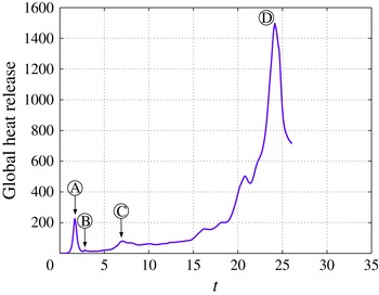
The global heat release rate for 2-D detonation initiation (
 $j_{max}=9$
) shows that several localized maxima occur after the initial power deposition and prior to the global heat release maximum.

As shown in figure 2, heat is deposited in a circle in the bottom left-hand corner from
 $0.5\leqslant t\leqslant 5.25$
. The initial rise time of the energy addition from the external source is short compared to the local acoustic time. Kassoy (Reference Kassoy2010) has shown that in this circumstance low Mach number gas expansion in the initially heated region is the source of mechanical disturbances (compression waves) that propagate into the neighbouring gas. In the first frame (
 $t=2$
), the compression wave, supported by continued energy deposition from the source until
 $t=5.25$
, and the burnt–unburnt gas interface, defined by
 $Y=0.5$
, share the same location, making it difficult to identify the compression wave from the material interface. It should be noted that the spatial distribution of
 $Y$
is continuous, while that for
 $T$
is continuous except at gasdynamic discontinuities. For later frames,
 $t\geqslant 4$
, the compression wave decouples from the propagating reaction zone, evolves into a shock, and propagates into the reactive mixture. Shock waves are identified in the temperature contour as abrupt jumps in temperature that increase the reactive mixture temperature to a value in the range 2–4 non-dimensional units (colour changes from black to dark red). Combustion product temperatures vary from
 $8$
to
 $12$
(orange to yellow), depending on how rapidly the mixture reacted and how much localized gas expansion acts as a heat sink. Fluid regions heated by the initial power deposition in addition to the chemical heat release have temperatures as high as
 $20$
or more (coloured white). Fluid that is undergoing active reaction will range in colour from dark red to orange.
Figure 3 plots the spatially integrated heat release (defined in (4.4)) as a function of time. Before
 $t=2$
, the reactants inside the deposition region are consumed in a chemical explosion, which adds additional heat to the deposition region. This heat release is seen as the first peak near
 $t=2$
(label A) in figure 3.
At some point shortly after
 $t=2$
when the compression waves first reflect off the left and bottom walls, the compression waves become fully discontinuous shock waves where the jump condition is resolved over just a few grid points. The reflected and transmitted shocks form Mach stems that propagate in the positive
 $x$
- and
 $y$
-directions. The reflected waves impinge on the burnt–unburnt gas interface and induce Richtmyer–Meshkov instabilities, which then increase the fluctuation magnitude at the material interface. This fluctuation can be initially observed in the
 $t=3.5$
contour near the left and bottom boundaries.
At approximately
 $t=2.5$
, a new localized reaction occurs in the lower left corner when the shock waves reflect off the bottom and left walls and raise the temperature and pressure in that region on a time scale similar to the local acoustic time. Clarke’s equation (Clarke Reference Clarke and Buckmaster1985) and a more generalized analogue (Kassoy Reference Kassoy2016) imply that all thermodynamic variables are coupled. The reactive gas ignites akin to an induction period process in a classical thermal explosion once it has reached a sufficient temperature. This phase of the reaction process consumes only a small amount of the remaining reactant, which makes the heat release transient barely visible in figure 3 at
 $t=2.5$
(label B) shortly after the first peak at around
 $t=2$
. A quantitative characterization of this hot spot explosion is described in the following section.
In the
 $t=5$
frame, the original outward propagating shock wave has reflected off the left and bottom walls and the Mach stems are visible in the temperature contour along the bottom and left boundaries. On the left wall, the leading edge of the shock wave is just about to reflect off the upper left corner. When reflection occurs on the upper boundary a rapid reaction process is initiated in the upper left-hand corner of the channel. The heat released in the hot spot is the source of a low Mach number local expansion process described in Kassoy (Reference Kassoy2010, Reference Kassoy2014b
) and Kurtz & Regele (Reference Kurtz and Regele2014a
), which is characterized by only partial local inertial confinement, where the pressure rises with temperature and a minor reduction in density. The heat released from this localized reaction process corresponds to the peak in heat release rate shown in figure 3 at
 $t=7.6$
(label C).
At
 $t=7$
, figure 2 shows that the reflected wave re-enters the reacted region and is refracted, which induces an additional longitudinal component to the wave direction. Obviously, the creation of additional longitudinal compression waves through transverse wave refraction inside the reacted fluid medium is a mechanism not present in the previous 1-D work (Kassoy et al.
Reference Kassoy, Kuehn, Nabity and Clarke2008; Regele Reference Regele2008; Regele et al.
Reference Regele, Kassoy and Vasilyev2012). The transverse waves compress and heat spatially distributed volumes of unreacted fuel (preconditioning), which ignite and help produce additional longitudinal waves, as well as sustaining the transverse waves that reflect off the top and bottom walls.
Kelvin–Helmholtz roll-up instabilities are clearly visible in frames
 $t=[10,12,14]$
at the burnt–unburnt gas interface with a fairly high level of detail. The existence of such a detailed interface serves as an indicator that numerical diffusion present in the algorithm has been minimized to the point that such structures can exist without immediately initiating a reaction in the unburnt reactant.
Figure 3 shows that the induction period phenomena (
 $2.5\leqslant t\leqslant 15$
) are replaced by much shorter time-scale heat addition beginning just before
 $t=20$
. The consequences of accelerated heat release can be observed in the temperature contour sequence beginning at approximately
 $t=14$
and ending at
 $t=24$
and in the global heat release profile (labelled D) with the formation of the over-driven detonation wave emerging from the lead shock front. It is speculated that only some of the spatially distributed, localized reaction processes evolve to the extremely rapid heat phase. Clearly the maximum at D in figure 3 confirms that sufficient spatially distributed heat release is the source of the induced gasdynamics observed in figure 6.
5.3 Detailed localized hot spot characterization
Figure 3 plots the spatially integrated heat release rate as a function of time. Four different localized explosions are highlighted as A, B, C and D. Of these four localized reactions, the first three indicate truly localized reactions where the heat release is fast enough to produce compression waves. The last maximum, D, is the result of an accelerating reaction front that ultimately culminates in an overdriven detonation wave.
The first localized explosion, A, occurs when the fuel located in the region that is heated by the thermal power deposition reacts. The reaction starts at
 $t=1.42$
and ends at
 $t=1.9$
. The temperature contour displayed in figure 2 at
 $t=2$
is the temperature profile just after the reaction has completed. The ratio of the heating to acoustic times can be calculated as
 $t_{h}/t_{a}$
, where
 $t_{h}$
is the heating time and
 $t_{a}$
is the acoustic time of the reaction region. The heating time is
 $t_{h}=1.9-1.42=0.48$
. The acoustic time is defined as the characteristic length-scale over the local sound speed
 $t_{a}=r_{A}/a_{0}$
, where
 $r_{A}=2$
is the radius of the fluid circle and
 $a_{0}$
is the ambient sound speed
 $a_{0}=\sqrt{T_{0}}$
. With the ambient temperature
 $T_{0}=1$
the acoustic time scale is
 $t_{a}=2/1=2$
, which gives a reaction to acoustic time scale ratio
 $t_{h}/t_{a}=0.24$
.
Since the time scale ratio is significantly less than unity, the reaction occurs under significant inertial confinement such that a low Mach number fluid motion is induced during the reaction (Kassoy Reference Kassoy2010). An isolated analysis has been performed by Kurtz and Regele in one (Kurtz & Regele Reference Kurtz and Regele2014a
) and two (Kurtz & Regele Reference Kurtz and Regele2014b
) dimensions to demonstrate this behaviour. Compression waves are emitted from the reaction region. These compression waves are visible as a faint red circle surrounding the reacted fluid region in figure 2 in the
 $t=3.5$
frame. Regele et al. (Reference Regele, Kassoy and Vasilyev2012) used
 $x$
–
 $t$
diagrams to illustrate 1-D detonation initiation from a similar thermal power deposition. It is possible to interpret the present 2-D data using
 $x$
–
 $t$
diagrams by reducing the data to 1-D in the
 $x$
-direction and averaging over the flow quantities in the
 $y$
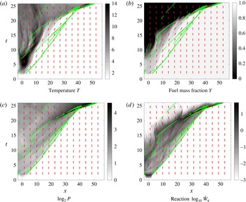
-direction. Figure 4 contains
 $x$
–
 $t$
contour plots of (a) temperature, (b) fuel mass fraction, (c) pressure (
 $\log _{2}P$
) and (d) chemical heat release rate (
 $\log _{10}{\dot{W}}q$
). Red arrows indicate qualitatively the spanwise average flow velocity in the
 $x$
-direction. Green dots/lines show areas where the mean velocity gradient
 $\text{d}\bar{u}/\text{d}x>0.07$
and indicate regions where compression/shock waves exist over a significant portion of the 2-D flow field. Here
 $\bar{u}$
indicates the spanwise averaged velocity where the average is evaluated in the
 $y$
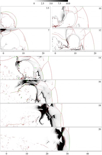
-direction. In the temperature contour shown in figure 4(a), the temperature increases start around
 $t=2$
between
 $-2\leqslant x\leqslant 2$
, which is after the reaction has completed. At the same time, the fuel mass fraction
 $x$
–
 $t$
contour also shows that some, but not all, of the fuel has been consumed in that region. In the pressure contour shown in figure 4(c), the pressure rises during the reaction and a compression wave, indicated by the green line, moves in the positive
 $x$
-direction away from the reaction region. Finally, the chemical heat release contour in figure 4(d) shows that a rapid reaction occurs during the chemical reaction near
 $t=2$
, but then the compression wave that is emitted away from the reaction source preconditions the gas to a higher temperature so that the entire fluid region behind it now has a finite induction period.
 $x$
–
 $t$
diagrams of the spanwise averaged (a) temperature, (b) fuel mass fraction
 $Y$
, (c) log base 2 of the pressure and (d) log base 10 of the heat of the reaction. Red arrows indicate flow direction and green dots are indications of discontinuous spanwise averaged velocity and pressure.

Explosion B occurs in the bottom left-hand corner of the domain during
 $2.64<t<2.88$
when the shock wave created from explosion A impacts the corner. Figure 2 shows that between the
 $t=2$
and
 $t=3.5$
frames, a small amount of fluid in the lower left corner has reacted. It should also be noted that there is not any reacted fluid touching the walls. The extra confinement from being inside a corner causes only this fluid to react and not the immediate surrounding areas along the walls. The radius of this fluid during the reaction is
 $R_{B}=0.2$
, which gives an acoustic time of
 $t_{a}=0.2/1=0.2$
. With the heating time
 $t_{h}=2.88-2.64$
the acoustic time scale ratio
 $t_{h}/t_{a}=1.2$
. As demonstrated in Kurtz & Regele (Reference Kurtz and Regele2014a
) and Kurtz & Regele (Reference Kurtz and Regele2014b
), this time scale ratio suggests that simultaneous compression and expansion occur during the fluid’s reaction, which ultimately produces a compression wave that propagates out radially from the bottom left corner. The impact of this compression wave is difficult to observe in the
 $x$
–
 $t$
diagram in figure 4 because the length scale of the reaction region is so small that the pressure drops very quickly and when averaged over the solution in the
 $y$
-direction it does not show a wave propagating in the positive
 $x$
-direction. Its source can be observed though at the left wall (
 $x=-3$
) where green dots are located at roughly
 $t\approx 3$
. The trajectory of this wave can be carefully traced by starting at these green dots and following the increase in temperature and reaction rate in figure 4(c,d).
At
 $t=5$
, figure 2 shows that the shock wave created from the initial explosion A is about to reflect off the top wall in the top left corner. After this reflection the temperature and pressure rise to create a localized reaction during
 $6.2<t<7.6$
. The characteristic length scale of this reaction is roughly
 $R_{C}=1$
. In this case, the reacting fluid is not symmetric (circular) and has some aspect ratio. The
 $t=7$
frame in figure 2 shows this reacting region of fluid is longer in the
 $x$
-direction than in the
 $y$
-direction. To remain consistent with the 2-D analysis performed in Kurtz & Regele (Reference Kurtz and Regele2014b
), the characteristic length scale of the shorter dimension is used to obtain the characteristic length scale. With the acoustic time still
 $t_{a}=1$
and the heating time
 $t_{h}=1.4$
, the heating to acoustic time scale ratio is
 $t_{h}/t_{a}=1.4$
. Again, this time scale ratio suggests that partial inertial confinement occurs during the reaction and compression waves can be expected to emerge from the localized reaction region. Close observation of the chemical heat release in figure 4(d) in the spatial region
 $-3\leqslant x\leqslant 0$
and temporally from
 $6\leqslant t\leqslant 7.6$
shows that the reaction rate has increased significantly in this region. A green line emerges from within this zone and propagates in the positive
 $x$
-direction. Subsequently, figure 4(b) shows that in the next few acoustic time units the fuel begins to burnout completely leaving zero reactants (
 $Y=0$
) along the left wall.
5.4 Accelerating reaction front characterization
Figure 3 shows that the global heat release after the localized explosion C is characterized by an induction period where the chemical heat release increases very slowly until approximately
 $t=15$
. At that point the global heat release begins to increase until the peak at D is reached. A few local maxima exist between C and D and indicate the chemical heat release from several different localized reactions. In fact, the entire process starting from approximately
 $t\approx 8$
until the peak at D is full of multiple localized reactions. It is extremely difficult to locate both the temporal and spatial boundaries of each of these reactions in figure 2. This makes it problematic to perform the same time scale analysis for the time following explosion C as for explosions A–C. A different approach is required.
The fuel mass fraction
 $x$
–
 $t$
diagram (figure 4
b) shows that starting at
 $t\approx 15$
a compression wave (indicated by a green line moving in the positive
 $x$
-direction) is approximately coincident with a rapid reduction in fuel mass fraction, with the final fuel mass fraction
 $Y=0$
. However, for this same green line in figure 4 the pressure remains relatively constant until
 $t\approx 18$
. The reaction of this fluid can be observed in figure 2 from frames
 $14<t<18$
where the volume of unreacted fluid located above the hot bubble of high-temperature gas is reacting steadily from left to right. This reaction wave is driven by auto-ignition of the reactants after the induction period set up by the compression waves from the localized reactions has elapsed.
One may be tempted at this point to attribute the behaviour of the accelerating reaction front to the Zeldovich (Reference Zeldovich1980) or SWACER mechanisms (Lee, Knystautas & Yoshikawa Reference Lee, Knystautas and Yoshikawa1978). However, the time scale analysis approach may still be applied in a novel way. Consider the trajectory of a spontaneous reaction front as illustrated in figure 4(b). Assume for the sake of simplicity that the trajectory is solely a function of the induction time
 $\unicode[STIX]{x1D70F}_{i}(x)$
and that the reaction duration is nearly instantaneous. Now consider a small fluid volume of characteristic length
 $\unicode[STIX]{x0394}x$
located at
 $x_{0}$
. The heat release time for this fluid volume occurs between
 $\unicode[STIX]{x1D70F}_{i}(x_{0})$
and
 $\unicode[STIX]{x1D70F}_{i}(x_{0}+\unicode[STIX]{x0394}x)$
. Thus, the heating time for the fluid volume
 $\unicode[STIX]{x0394}x$
is
 $$\begin{eqnarray}t_{h}=\unicode[STIX]{x1D70F}_{i}(x_{0}+\unicode[STIX]{x0394}x)-\unicode[STIX]{x1D70F}_{i}(x_{0}).\end{eqnarray}$$
The ignition delay time
 $\unicode[STIX]{x1D70F}_{i}(x_{0}+\unicode[STIX]{x0394}x)$
can be expanded using a Taylor series expansion to obtain
 $$\begin{eqnarray}t_{h}=\frac{\text{d}\unicode[STIX]{x1D70F}_{i}(x_{0})}{\text{d}x}\unicode[STIX]{x0394}x+O(\unicode[STIX]{x0394}x^{2}).\end{eqnarray}$$
The acoustic time scale for the same fluid volume is
 $t_{a}=\unicode[STIX]{x0394}x/a(x_{0})$
, where
 $a(x_{0})$
is the sound speed at
 $x_{0}$
. The heating to acoustic time scale ratio can then be evaluated to be
 $$\begin{eqnarray}\frac{t_{h}}{t_{a}}=\frac{\text{d}\unicode[STIX]{x1D70F}_{i}(x_{0})}{\text{d}x}\frac{\unicode[STIX]{x0394}x}{\unicode[STIX]{x0394}x/a(x_{0})}=\frac{a(x_{0})}{u_{s}(x_{0})},\end{eqnarray}$$
where
 $u_{s}$
is defined to be the spontaneous wave speed
 $u_{s}=(\text{d}\unicode[STIX]{x1D70F}_{i}/\text{d}x)^{-1}$
(Zeldovich Reference Zeldovich1980). The result is that the ratio of the heating to acoustic time is equal to the inverse of the ratio of the spontaneous wave speed to local sound speed.
Acoustic time scale characterization has demonstrated (Kassoy Reference Kassoy2010; Regele et al.
Reference Regele, Kassoy and Vasilyev2012; Kurtz & Regele Reference Kurtz and Regele2014a
,Reference Kurtz and Regele
b
) that when a volume of fluid reacts quickly such that
 $t_{h}/t_{a}\ll 1$
the fluid reacts in a nearly constant volume process. Equation (5.6) shows that for a small time scale ratio the spontaneous wave speed is much larger than the local sound speed,
 $u_{s}\gg a$
, which corresponds to a weak detonation or Case 1 in Zeldovich (Reference Zeldovich1980). Kassoy (Reference Kassoy2016) has demonstrated analytically that a spontaneous reaction wave with
 $t_{h}/t_{a}\ll 1$
propagates at a supersonic velocity. On the opposite end of the spectrum, if
 $t_{h}/t_{a}\gg 1$
the fluid reacts slowly enough that the pressure is able to equalize and a nearly constant pressure reaction occurs (Kurtz & Regele Reference Kurtz and Regele2014a
,Reference Kurtz and Regele
b
). Equation (5.6) shows that this condition corresponds to the situation when the spontaneous wave speed is slow in comparison to the sound speed
 $u_{s}\ll a$
, which is condition 3 in Zeldovich (Reference Zeldovich1980). Finally, if
 $t_{h}/t_{a}\approx 1$
, compression waves are generated simultaneously with fluid expansion and an
 $O(1)$
induced Mach number is observed (Kassoy Reference Kassoy2010; Kurtz & Regele Reference Kurtz and Regele2014a
,Reference Kurtz and Regele
b
; Kassoy Reference Kassoy2014a
, Reference Kassoy2016). This corresponds to condition 2 in Zeldovich (Reference Zeldovich1980) where
 $u_{s}\lesssim u_{J}$
. In other words, the acoustic time scale characterization approach developed using Kassoy’s asymptotic analyses (Kassoy Reference Kassoy2010, Reference Kassoy2016) provides a formal mathematical foundation for the Zeldovich mechanism.
Identification of the heating to acoustic time scale ratio is difficult using the localized analysis approach performed for localized reactions A–C. However, through the use of (5.6), the spontaneous wave speed and local sound speed can easily be computed to determine the evolving heating to acoustic time scale ratio that describes the heat release events leading up to the global heat release peak D in figure 3. The wave speed
 $u_{s}$
is determined by tracking the locations (
 $x_{1/2}$
) where half of the fuel has been consumed
 $Y=0.5$
. There are often multiple locations where
 $Y=0.5$
. In order to obtain a single value the average location
 $\bar{x}_{1/2}$
at each time is used to track the reaction wave front. A low pass smoothing filter is then applied and the derivative can be evaluated to give the spontaneous wave speed
 $u_{s}=\text{d}\bar{x}_{1/2}/\text{d}t$
. The average local sound speed
 $\bar{a}$
is computed in a similar manner.
Based upon the fuel mass fraction plot in figure 4(b), the planar-averaged fuel mass fraction does not drop below
 $Y=0.5$
until
 $t\gtrsim 10$
. Thus, in order to focus on the evolution of the spontaneous reaction following explosions A–C, the time scale ratio
 $t_{h}/t_{a}=\bar{a}/\bar{u}_{s}$
is evaluated for
 $t\geqslant 11$
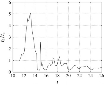
. Figure 5 shows the heating to acoustic time scale ratio
 $t_{h}/t_{a}$
for the times leading up to the global maximum in heat release D at
 $t=24$
. From
 $11\leqslant t\leqslant 14.5$
, the time scale ratio starts near unity, rises as high as five, and then falls below unity thereafter. Expansion of the reacted gases (
 $Y=0$
) in figure 4(b) shows that this period is associated with fluid expansion after explosion C completed. The interface at
 $Y=0.5$
moves to the right and the slope steepens as the pressure distribution is homogenized. Figure 5 shows that during this time period the time scale ratio is significantly above unity, which indicates that the fluid is free to expand and the pressure is being homogenized. This can be further verified by looking at the pressure in figure 4(c) in this region.
As indicated by the change in trajectory of the burnt–unburnt gas interface in figure 4(b), at
 $t\approx 15$
a spontaneous chemical reaction wave (Zeldovich Reference Zeldovich1980; Kassoy Reference Kassoy2016) develops and propagates to the right. The green line indicates that compression in the fluid accompanies this wave. This wave can be observed in figure 2 as the rapidly evolving reaction front located above the bubble of hot reacted material in frames 14–20. Figure 5 shows that during most of this time the heating to acoustic time scale ratio is less than unity
 $t_{h}/t_{a}<1$
. There are a couple of occasions where the time scale ratio is greater than unity. These fluctuations are associated with the fact that this spontaneous wave is made up of numerous pockets of fluid of different sizes reacting at different times, all of which contribute to the reaction wave.
Heating to acoustic time scale ratio
 $t_{h}/t_{a}$
for the time leading up to the formation of the detonation.

For
 $20\geqslant t\geqslant 24$
the size of the localized reactions becomes larger and the number fewer such that the magnitude of the fluctuations in
 $t_{h}/t_{a}$
is smaller and the number of fluctuations is fewer. The time scale ratio fluctuates less during this period, which indicates that the evolving wave is becoming quasi-steady. Figure 4(c) shows that the pressure during this time period really begins to increase at the wave front, which demonstrates that the reaction is coupling with a preceding compression wave and explains the increase in regularity. There is a drop in
 $t_{h}/t_{a}$
at
 $t=24$
. This corresponds to the emergence of the detonation wave into the cooler undisturbed reactive fuel mixture. At this point, the local sound speed is lower, which accounts for the momentary drop in the time scale ratio. The time scale ratio increases slightly to a more steady value once the wave has completed its transition into the cooler medium.
The sequence of temperature contours for
 $j_{max}=[7,8,9]$
shows that while the fine-scale structures increase in complexity, the differences in large gasdynamic structures decrease with each increase in resolution.

The 2-D behaviour observed here is very similar to previous 1-D studies using thermal power deposition to initiate detonation waves (Sileem et al.
Reference Sileem, Kassoy and Hayashi1991; Kassoy et al.
Reference Kassoy, Kuehn, Nabity and Clarke2008; Regele et al.
Reference Regele, Kassoy and Vasilyev2012). Multiple localized hot spot reactions contribute to preheating the reactive gas until a final explosion occurs in the form of a spontaneous wave. Kassoy (Reference Kassoy2016) has modelled this process in terms of a propagating thermal explosion, which defines the spontaneous wave propagation process. While there are multiple localized explosions that occur with heating to acoustic time scale ratios
 $t_{h}/t_{a}=O(1)$
, there are many more that react more slowly and do not contribute much to the overall induced fluid motion. In order to demonstrate the similarity between 1-D and 2-D thermally initiated acoustic time scale thermal power deposition it is important to fully resolve the auto-ignition time of all pockets so that a solution is obtained that is independent of resolution and solely dependent on gasdynamic effects.
5.5 Resolution dependence
A purely gasdynamic detonation initiation solution is sought by increasing the level of resolution until it appears that the initiation process converges as measured quantitatively by the global heat release profile. Since the Euler equations are solved, there is no predefined length scale to resolve and the fine-scale structure detail increases indefinitely with resolution. Since a reaction source term introduces a time scale, the spatially integrated chemical heat release is used to indicate convergence. However, since the scale is introduced through a reaction source term without any diffusion defined scales, strong dependence on numerical resolution is anticipated up to the point when all scales related to gasdynamic effects are resolved.
5.5.1 Large- and small-scale comparison
Figure 6 shows a sequence of temperature contours for the highest resolution (
 $j_{max}=7$
,
 $8$
and
 $9$
) cases. In order to compare the three cases, it is informative to focus on the evolution of large (integral) and small (finest level of resolution) flow structures. In particular, while the scale of the smallest observed structures decreases with the increase of the resolution, the large-scale gasdynamic structures qualitatively remain unchanged. Furthermore the small-scale structures seen near the wall at
 $x=-3$
exist in a previously burned out region and cannot add to the global heat release.
Between the three cases for
 $0<t<10$
, there is little noticeable difference in the large-scale gasdynamic structures such as the lead shock front and location of the burnt–unburnt gas interface. As expected, differences between these three cases exist in the fine scale structures during this initial period. For
 $t>10$
, the volume of hot combustion products present in the lower resolution case
 $j_{max}=7$
increases with time more quickly than the other two higher-resolution cases. This indicates that the lack of resolution in the
 $j_{max}=7$
case artificially accelerates the rate of detonation formation.
Up until the last frame, only minor differences in the large-scale gasdynamic structures exist between the
 $j_{max}=8$
and
 $j_{max}=9$
cases. The vortical structures near the closed end of the channel show a significant difference on the finer scales. However, it is only between
 $22<t<24$
that there is a notable difference in the large gasdynamic structure characterized by the different detonation formation times. Continued resolution may show larger differences in the fine-scale features, but even smaller differences in the large gasdynamic structures.
5.5.2 Global convergence
In order to illustrate the dominance of gasdynamic effects on the global physical quantities, it is illustrative to examine grid dependence using spatially integrated quantities, such as the spatially integrated heat release defined in (4.4). This approach has the same effect as the error norms, but provides a bit more insight into the fundamental physics driving detonation formation and evolution. It is also a more intuitive approach in the absence of an exact solution.
Figure 7 plots the spatially integrated heat release rate for the five different levels of grid resolution
 $j_{max}=[5,6,7,8,9]$
. Each curve shows the same general features, such as the initial power deposition peak, explosions in the bottom left and top left corners, and a period of rapid fuel consumption followed by the formation of an over-driven detonation wave. The global maximum indicates a large consumption of fuel in a short period of time and coincides approximately with the formation of the over-driven detonation wave. The time corresponding to the global maximum of the heat release curve will be referred to as the detonation formation time (DFT).
Heat release profiles for the five different levels of resolution. The differences between each successive profile diminish with increasing resolution.

Unlike the 1-D results in figure 1, figure 7 shows that the global heat release profiles vary widely with resolution for
 $5\leqslant j_{max}\leqslant 7$
, In fact, for the
 $j_{max}=5$
case, the detonation formation time is approximately half that of the high-resolution cases,
 $j_{max}=8$
and
 $9$
. The variance between each curve becomes less noticeable as the resolution increases. This indicates that the spatially integrated heat release becomes less dependent on the grid spacing and numerical diffusion as the resolution is increased. Convergence appears to occur for
 $j_{max}\geqslant 8$
. This suggests that the 2-D spatial temperature distribution
 $T(t,\boldsymbol{x})$
is sensitive to resolution as demonstrated in figure 6.
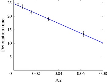
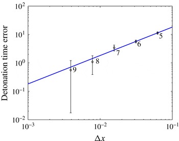
The detonation formation times can be estimated from the global maxima of the heat release in figure 7. Since the detonation is not necessarily formed at the peak of the heat-release curve, some uncertainty exists in the DFT valuation. Consequently, the width of the peak at half its maximum is used as an uncertainty in obtaining the DFT. Figure 8 plots the DFTs as a function of the minimum grid spacing for each level of resolution on a linear scale. The detonation time increases linearly with decreased grid spacing. This is expected as the numerical algorithm is first-order accurate at the burnt–unburnt gas interface as well as shocks.
The convergence rate for 2-D detonation initiation is linear. The extrapolation line indicates that finer resolution will increase the peak heat release time by less than
 $5\,\%$
.

Figure 8 shows that the difference in detonation formation time between the
 $j_{max}=8$
and
 $9$
cases is within the error of estimation. Extrapolation of the linear curve gives a detonation formation time of
 $t_{0}=24.7$
for infinite resolution (
 $\unicode[STIX]{x0394}x\rightarrow 0$
). This time can be used as a value for comparison of the DFT error, defined to be
 $\unicode[STIX]{x1D6FF}=t-t_{0}$
. Figure 9 plots this error as a function of
 $\unicode[STIX]{x0394}x$
on a standard log–log scale. It shows that the error is indeed a linear function of the grid spacing.
The error between the extrapolated detonation time and the detonation time at a given grid resolution shows a linear dependence on grid spacing.

Surface length of
 $Y=0.5$
contour as a function of time, ultimately converging to the size of the channel.

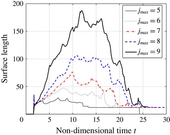
Figures 8 and 9 show convergence of the DFT. It is important to note that while the integrated global quantities such as DFT converge with the increase of resolution, no point-wise convergence of the local quantities can be observed due to the progressive appearance of the small-scale flow structures, which can have only minor impact on the global heat release. In order to illustrate both simultaneous convergence of the DFT and a lack of point-wise convergence, the surface of the burnt–unburnt gas interface (defined as
 $Y=0.5$
) can be integrated to obtain the surface length at this interface. Figure 10 plots the surface length as a function of time for the five different levels of resolution. The surface length is initially identical for each case, but continues to grow at different rates. As expected, the growth rate of the surface length increases with the increase of the level of resolution. At some point the growth rate is reduced until the surface length reaches a maximum. Subsequently, the surface length decreases until it reaches a value of approximately
 $12$
, which corresponds to the surface length of the detonation wave (i.e. roughly the channel height). The surface length reaches its minimum value at roughly the same time (approximately
 $t=25$
) for the
 $j_{max}=8$
and
 $9$
cases. This is a slightly later time than that observed from the peak heat release times shown in figure 7. The peak heat release time generally occurs prior to the minimum surface length time because the peak heat release corresponds to a large volume of gas reacting at once that then facilitates the final formation of the detonation wave.
It is clear from figure 10 that there is indeed no point-wise convergence of the burnt–unburnt gas surface length during the evolution of the detonation wave. However, the temporal convergence of the detonation formation times in both the global heat release (figure 7) and the surface length (figure 10) suggest that larger global scales exist that dominate the detonation formation behaviour. Thus, the evolution of the detonation waves in the high-resolution cases (
 $j_{max}\geqslant 8$
) is independent of the effects of any fine-scale structures. This makes sense because in the context of the original assumption that viscous/diffusive transport effects can be considered negligible, it follows that the only physical scale that must be resolved is the reaction time. In this way, the behavioural description from the 1-D studies with the Euler equations (Sileem et al.
Reference Sileem, Kassoy and Hayashi1991; Regele et al.
Reference Regele, Kassoy and Vasilyev2012) is successfully extended to this 2-D case.
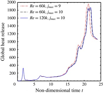
In order to further support the conclusion that the detonation initiation process illustrated here is independent of diffusive/viscous effects, three additional simulations using the NS equations are performed. Two of the simulations are based on acoustic Reynolds numbers
 $Re_{a}=60\,000$
at two different resolution levels
 $j_{max}=9$
and
 $10$
, and the third simulation is at twice the acoustic Reynolds number
 $Re_{a}=120\,000$
. The two simulations at the same Reynolds numbers
 $Re_{a}=60\,000$
show very similar surface perturbation wavelengths and amplitudes, despite being resolved at two different resolutions. The DFT for the higher resolution case is slightly longer than the lower resolution case, which is attributed to the fact that there is still some artificial viscosity present that is lower in the higher resolution case. The higher Reynolds number case
 $Re_{a}=120\,000$
shows a distinct change in surface instability behaviour. In particular, the wavelength is roughly half that of the lower Reynolds number case. However, the global heat release for this case is almost exactly that of the higher resolution
 $Re_{a}=60\,000$
case, which indicates that the global heat release is independent of both artificial and molecular diffusion. These results show that the convergence of the global heat release in the Euler simulations is also observed with the NS equations. Full details of the NS results may be found in the Appendix.
6 Discussion
The DDT process outlined in this work is shown to occur independent of diffusive effects. This is demonstrated by increasing the resolution of Euler simulations until the global heat release becomes independent of resolution. Additional simulations using the NS equations verify that given a sufficiently large acoustic Reynolds number the heat release becomes independent of resolution as well as molecular diffusion. This demonstrates that the detonation initiation sequence presented here is a function primarily of the large-scale gasdynamic structures. Since large-scale structures react within a volume undergoing a relatively gentle induction period reaction followed by an ‘explosive’ event on a much shorter time scale (Kassoy Reference Kassoy2016) through volumetric auto-ignition, fine-scale structures associated with the burnt–unburnt gas interface do not contribute much to the global heat release.
As numerical diffusion decreases, the surface length of the material interface (figure 10) grows more rapidly. The contour plots (figure 2) for the cases
 $j_{max}=8$
and
 $9$
show the generation of both Richtmyer–Meshkov and Kelvin–Helmholtz instabilities for high enough resolution. This is consistent with previous simulations using adaptive grid codes that solve the Euler equations with premixed reactants (Fryxell et al.
Reference Fryxell, Olson, Ricker, Timmes, Zingale, Lamb, Macneice, Rosner, Truran and Tufo2000; Deiterding Reference Deiterding2009; Seitenzahl et al.
Reference Seitenzahl, Meakin, Townsley, Lamb and Truran2009; Ziegler et al.
Reference Ziegler, Deiterding, Shepherd and Pullin2011).
The detonation initiation process presented here is similar to the reinitiation of detonation waves after passing through perforated plates (Zhu, Chao & Lee Reference Zhu, Chao and Lee2007) or columns of cylinders (Radulescu & Maxwell Reference Radulescu and Maxwell2011; Maley et al. Reference Maley, Bhattacharjee, Lau-Chapdelaine and Radulescu2015). In both cases, a strong shock wave passes into the unburnt material and preconditions the gas. However, in the experiments performed by Radulescu & Maxwell (Reference Radulescu and Maxwell2011), regions of high exothermicity are observed in open-shutter photographs suggesting that heat release from a turbulent flame front may be contributing to the reinitiation process. Additionally, in highly unstable detonation waves, there is considerable evidence to suggest that the large unreacted pockets of fluid downstream of the detonation front are consumed (Austin, Pintgen & Shepherd Reference Austin, Pintgen and Shepherd2005; Radulescu et al. Reference Radulescu, Sharpe, Lee, Kiyanda, Higgins and Hanson2005, Reference Radulescu, Sharpe, Law and Lee2007; Kiyanda & Higgins Reference Kiyanda and Higgins2013) through strong turbulent surface reactions rather than auto-ignition. However, these other behaviours can only be compared to the current results in a limited capacity. What these other processes possess that the current case lacks is a continuous jetting effect. The thermal power deposition in this work provides a thermomechanically driven piston effect analogous to the jetting in these other cases. However, the duration of the piston effect is much shorter than the jetting in these other cases, which makes shock waves and thus the shear layers in the present work much weaker than those seen in the other situations. While the current process appears to be independent of transport effects this does not imply that the other cases will be as well.
Romick et al. (Reference Romick, Aslam and Powers2012) and Romick, Aslam & Powers (Reference Romick, Aslam and Powers2015) show that detonation dynamics in one dimension are influenced by viscosity and inviscid cases lead to chaos more quickly than viscous cases. It is also found that the transition to chaos is a function of activation energy and the transitional activation energy is moderately sized (
 $E=E^{\prime }/(R^{\prime }T_{0}^{\prime })\sim 25$
). It should be pointed out that both the 1-D and 2-D results contained in this work focus on small activation energies in which case the instabilities observed in Romick et al. (Reference Romick, Aslam and Powers2012) and Romick et al. (Reference Romick, Aslam and Powers2015) may be absent.
In typical DDT processes turbulent flow conditions increase the reaction zone surface area such that compression waves propagate into the unreacted reactive mixture, precondition the fluid to create localized hot spots that explode and facilitate the formation of a detonation wave (Oppenheim & Soloukhin Reference Oppenheim and Soloukhin1973; Khokhlov & Oran Reference Khokhlov and Oran1999; Gamezo et al. Reference Gamezo, Ogawa and Oran2008; Ivanov et al. Reference Ivanov, Kiverin and Liberman2011). In this conventional approach viscous and diffusive transport effects play an important role during the early stages when the heat release is dominated by surface reactions from a flame. The purely gasdynamic detonation initiation process presented here retains much of the behaviour contained in typical DDT processes with turbulent flow conditions that increase the burnt–unburnt gas interface. However, the DDT process in this work is not dependent on heat released from surface reactions and relies solely on gasdynamic heating and auto-ignition following an extended induction period. Purely gasdynamic detonation initiation is usually associated with direct initiation where the detonation is initiated with a strong blast wave. In this case, the initial power deposition of heat on the acoustic time scale is more subtle and creates a detonation initiation process that has the purely gasdynamic characteristics of direct initiation, but demonstrates evolutionary behaviour similar to conventional DDT where viscous and diffusive transport effects are considered highly important.
7 Conclusions
Two-dimensional simulations using the reactive Euler equations feature deposition of energy in a circular area of fluid during a finite time on the order of the acoustic time scale of the heated volume. Four localized hot spot explosions are identified in the detonation initiation process with the first being initiated by the initial thermal power deposition. Acoustic time scale analysis is used to characterize the thermomechanical response of the surrounding fluid to these reactions. The first three are easily characterized using traditional techniques where the size and duration of the localized explosion is obvious. The fourth explosion is a culmination of several localized explosions where their spatial and temporal boundaries are not easily identifiable. For this case, the acoustic time scale analysis approach is used in a novel way by showing that the time scale ratio becomes identical to the inverse ratio of the spontaneous wave speed and speed of sound. For this final explosion, the heating to acoustic time scale ratio rises well above unity during an induction period. Then large portions of fluid begin to react and cause the time scale ratio to fluctuate in the subunity range, which indicates that the explosions are inertially confined and strong compression waves will be emitted from the reaction region. A detonation wave forms after this final series of explosions is complete.
The simulations demonstrate that once the reaction zones are spatially resolved, it is possible to achieve purely gasdynamic detonation initiation, where a majority of the chemical heat is released through auto-ignition after an extended induction period. This claim is validated by demonstrating the convergence of various integral quantities such as the detonation formation times and integral heat release. It is shown that the convergence in two dimensions occurs much more slowly than in one dimension.
The evolving 2-D detonation initiation process contained in this work appears to contain all of the traditional characteristics of classical DDT where turbulent flow conditions lead to a burnt–unburnt gas interface with high surface area. However, in contrast to much of the recent detonation literature illustrating the importance of turbulent reactions, the heat release contained in this work is only from auto-ignition and is independent of surface reactions. In this respect, the behaviour is more similar to direct initiation from a blast wave. While the acoustic time scale detonation initiation process demonstrated in this work exhibits behaviours that are characteristic of classical DDT where viscous and diffusive transport effects are highly important, the evolutionary behaviour shown here is dependent only upon the large gasdynamic heating mechanisms, which is typically more characteristic of a direct initiation process.
Acknowledgements
This work was supported in part by the National Science Foundation under grant no. ACI-0242457 and by the Air Force Office of Scientific Research through subcontract 2012-2756 from the University of California, Irvine. D.R.K thanks the principal investigator Professor William Sirignano and program manager Dr M. Birkan for their encouragement as well as the late J. F. Clarke for inspiring discussions in the past that were influential in this work. O.V.V. acknowledges partial support by the Polish National Center of Science (NCN) project DEC 2013/10/M/ST6/00531. J.D.R. would like to thank G. Blanquart for the use of his computational resources in performing the simulations contained in this work.
Appendix
In order to demonstrate that the Euler solutions accurately capture the reactive flow physics, three additional cases were studied using the non-dimensionalized reactive NS equations (2.1) in the limit of large Reynolds numbers. The first case is identical to the inviscid case described in § 5.1 at the highest resolution (
 $j_{max}=9$
), but with a constant molecular viscosity, Prandtl (
 $Pr=1$
) and Schmidt (
 $Sc=1$
) numbers, and finite Reynolds number
 $Re_{a}=60\,000$
based on the channel height. The Reynolds number was chosen to be sufficiently high to minimize viscous dissipation and diffusion in the reaction zones. The second case also uses a Reynolds number
 $Re_{a}=60\,000$
, but is solved on a grid with twice the effective resolution (
 $j_{max}=10$
). The third case is solved with
 $Re_{a}=120\,000$
and at the higher resolution
 $j_{max}=10$
, corresponding to the effective resolution of 30 720
 $\times$
6144.
Note that despite the fine mesh used in the simulations, the resolution is still sufficiently larger than the
 $O(l^{\prime }Kn)$
required to resolve the physical thickness of the strong shock waves observed in the solution. In order to keep the computational cost somewhat manageable, the shock capturing scheme of Regele & Vasilyev (Reference Regele and Vasilyev2009) was used to thicken the strong shocks. It should be emphasized that numerical viscosity is only used in the neighbourhood of the shock waves and automatically switches off away from them. To demonstrate the localized nature of the shock capturing scheme and, more importantly, its negligible effect on the heat release, the reaction rate is shown in figure 11 at different instances of time for the
 $Re_{a}=120\,000$
and
 $j_{max}=10$
case. The reaction rates are superimposed with the contour plots of non-dimensional numerical viscosity at
 $\unicode[STIX]{x1D708}_{n}=Re_{a}^{-1}$
and
 $\unicode[STIX]{x1D708}_{n}=0.1Re_{a}^{-1}$
. As can be clearly seen, there are only a few locations on
 $t=14$
and
 $16$
plots where the artificial viscosity is greater than the molecular viscosity (green areas) in a region of reacting fluid where the shock wave passes through the reacting region. These results suggest that for these high-resolution cases the numerical diffusion has minimal impact on the reaction rate through localized transport effects (conduction and species diffusion).
Sequence of reaction rates for the NS cases at
 $Re_{a}=120\,000$
with effective resolution of 30 720
 $\times$
6144 superimposed with the contour plots of non-dimensional numerical viscosity at
 $\unicode[STIX]{x1D708}_{n}=Re_{a}^{-1}$
(green) and
 $\unicode[STIX]{x1D708}_{n}=0.1Re_{a}^{-1}$
(red). The reaction rates are shown in greyscale. The corresponding non-dimensional times are shown in the top right corner of each plot.

Sequence of temperature contours for the three NS cases.

Figure 12 shows a sequence of temperature contours for the three NS solutions. It can be seen that all three cases exhibit gasdynamic behaviour similar to that in the Euler solutions leading up to detonation formation. The first two columns describe the
 $Re_{a}=60\,000$
solutions for two different grid resolutions. The two columns are nearly identical until approximately
 $t=10$
, after which some notable qualitative differences can be observed along the edge of the hot gas bubble and the hot vortices in the burned out gases near the left boundary. The large-scale gasdynamic features are very similar with the primary difference being that the
 $j_{max}=9$
case shows that the detonation appears slightly earlier than the
 $j_{max}=10$
case, as indicated by the detonation structure observed in the
 $t=22$
frames. This is attributed to the fact that artificial viscosity is still present in the numerical algorithm to capture discontinuities in the solution such as shock waves, but as discussed above, it is relatively small at the burnt–unburnt gas interface in comparison to the molecular diffusion.
The third column of figure 12 shows results for a Reynolds number that is twice as large as the second case, and thus has half the viscosity and diffusion. It can be readily seen that the surface instability wavelength has decreased in the higher Reynolds number case as early as
 $t=7.5$
and continues until
 $t=12$
. In the
 $t=14$
contour the wavelength becomes more similar and beyond that time the gas surrounding the hot gas bubble reacts at approximately the same time as the
 $Re_{a}=60\,000$
case. The large-scale gasdynamic structures are nearly identical and the two
 $j_{max}=10$
cases detonate at almost exactly the same time.
Figure 13 shows the spatially integrated heat release as a function of time for the three different NS solutions. It can be seen that for the
 $Re_{a}=60\,000$
cases the higher-resolution case (
 $j_{max}=10$
) has a slightly longer detonation formation time than the lower-resolution
 $j_{max}=9$
case, which is consistent with the temperature contours observed in figure 12. This difference suggests that some grid dependence still exists between the two solutions. The heat release for the two
 $j_{max}=10$
cases is nearly identical. In fact there is only a barely noticeable lag in the heat release rate in the
 $Re_{a}=120\,000$
case compared to the
 $Re_{a}=60\,000$
case. This suggests that the detonation formation time is now independent of both the physical and numerical diffusion terms combined. As mentioned above, there is a noticeable difference in surface instability wavelength between these two different Reynolds number cases. However, the heat release is nearly identical. This suggests that the consumption of the fuel is dominated by auto-ignition following preconditioning from shock-wave compression, which is consistent with the solution behaviour obtained using the Euler equations.
Spatially integrated heat release for the three NS cases.