1. Introduction
It is well known that the classic transition route via the exponential growth of the Tollmien–Schlichting (TS) waves can be altered by free-stream noise as well as localised disturbance such as surface roughness elements and plasma actuations. When the boundary layer flow impinges on a three-dimensional (3-D) roughness element, a counter-rotating streamwise vortex pair (CRP) develops downstream of the roughness. The interaction between the CRP and the boundary-layer shear gives rise to streamwise-elongated velocity streaks via the lift-up mechanism. The development of such disturbance into transition bypasses the modal growth of the TS waves and is termed bypass transition. Bypass transition in the presence of surface roughness elements has been widely investigated both experimentally (White Reference White2002; Downs & White Reference Downs and White2008; Puckert & Rist Reference Puckert and Rist2018, Reference Puckert and Rist2019) and numerically (Loiseau et al. Reference Loiseau, Cherubini, Robinet and Leriche2014; Goldstein, Chu & Brown Reference Goldstein, Chu and Brown2017; Bucci et al. Reference Bucci, Puckert, Andriano, Loiseau, Cherubini, Robinet and Rist2018; von Deyn et al. Reference von Deyn, Forooghi, Frohnapfel, Schlatter, Hanifi and Henningson2020). In this work, we numerically study the influences of wall-normal vibration on the flow development and bypass transition downstream of an isolated roughness element, which will shed light on the transition over vibrating rough surfaces frequently encountered in engineering applications.
1.1. Bypass transition
The formation of streamwise-elongated velocity streaks represents the early stage of bypass transition. When the boundary-layer flow is subject to free-stream turbulence, low-frequency perturbations enter the boundary layer through shear sheltering (Hunt & Durbin Reference Hunt and Durbin1999) and tilt the base shear via the lift-up mechanism (Landahl Reference Landahl1980). In this process, the streamwise vorticity perturbations displace the low-momentum (high-momentum) fluid upwards (downwards), leading to the formation of low- and high-speed streaks of streamwise velocity, respectively. From a theoretical point of view, the generation and growth of boundary-layer velocity streaks can be linked to the transient growth of perturbations. Using linear transient growth analyses, researchers found that the optimal perturbation leading to the maximum transient growth consists of a pair of steady streamwise-aligned vortices (Butler & Farrell Reference Butler and Farrell1992; Andersson, Berggren & Henningson Reference Andersson, Berggren and Henningson1999; Monokrousos et al. Reference Monokrousos, Åkervik, Brandt and Henningson2010).
After generation, the streaks interact with the streamwise vorticity and the low- (high-) speed streaks are convected away from (towards) the wall via a nonlinear lift-up mechanism, resulting in an inflectional velocity profile that is prone to secondary instabilities (Mao et al. Reference Mao, Zaki, Blackburn and Sherwin2017). There are two types of secondary instabilities of streaks: sinuous and varicose (Swearingen & Blackwelder Reference Swearingen and Blackwelder1987). The sinuous mode features an asymmetric pattern with respect to the unstable velocity streak, whereas the varicose type presents a symmetric pattern. The sinuous instability normally occurs around the low-speed streak that is lifted to the top of the boundary layer and is associated with a spanwise inflectional velocity profile (Schlatter et al. Reference Schlatter, Brandt, de Lange and Henningson2008). The varicose counterpart, generally found in the overlapping region between the low- and high-speed streaks, is linked to an inflectional velocity profile in the wall-normal direction (Vaughan & Zaki Reference Vaughan and Zaki2011).
1.2. Roughness-induced instability
In addition to free-stream turbulence, the low-frequency disturbance can also be introduced by 3-D roughness elements, which develops into bypass transition downstream (von Doenhoff & Baslow Reference von Doenhoff and Baslow1961; Tani Reference Tani1969). A Reynolds number  $Re_k=U_k\, k/\nu$ based on the kinematic viscosity
 $\nu$, the roughness height
 $k$ and Blasius velocity at the top edge of the roughness
 $U_k$ is used to parametrise the onset of roughness-induced bypass transition. For example, the transition Reynolds number is between 600 and 900 when the aspect ratio of roughness equals to 1 (von Doenhoff & Baslow Reference von Doenhoff and Baslow1961). However, the physical mechanisms that lead to transition were not revealed in these early works. For an isolated roughness element, researchers observed a CRP in the low-speed region downstream of the element (Gregory & Walker Reference Gregory and Walker1955; Mochizuki Reference Mochizuki1961; Acarlar & Smith Reference Acarlar and Smith1987). When the roughness is sufficiently high in the wall-normal direction, the CRP develops into a hairpin vortex in the aft recirculation zone. As mentioned before, due to the lift-up effect (Landahl Reference Landahl1980), the CRP experiences strong transient growth, which then leads to the formation of velocity streaks. Therefore, the effects of roughness on bypass transition are linked to the transient growth theory in later works (Reshotko Reference Reshotko2001; White Reference White2002; White, Rice & Ergin Reference White, Rice and Ergin2005; Denissen & White Reference Denissen and White2013), and experimental findings also support the significance of transient growth in the roughness-induced transition in boundary-layer flow (Downs & White Reference Downs and White2008). Recently, von Deyn et al. (Reference von Deyn, Forooghi, Frohnapfel, Schlatter, Hanifi and Henningson2020) investigated the coupling effect of free-stream turbulence and distributed roughness and found out that their combination results in amplified streaks, and thus earlier bypass transition.
When the non-parallel wake zone is taken into consideration, 3-D global instability analyses show that the central low-speed region downstream of an isolated roughness element supports two types of global instabilities: a sinuous mode and a varicose mode (Loiseau et al. Reference Loiseau, Cherubini, Robinet and Leriche2014), similar to the instability of velocity streaks caused by free-stream disturbance. These instability modes are also observed by Puckert & Rist (Reference Puckert and Rist2018) in experiments. The varicose instability is more common and is the dominant mode at subcritical Reynolds numbers (Bucci et al. Reference Bucci, Puckert, Andriano, Loiseau, Cherubini, Robinet and Rist2018). In compressible flow, De Tullio et al. (Reference De Tullio, Paredes, Sandham and Theofilis2013) found that the roughness wake consists of a low-speed streak, leaving the 3-D shear layer highly unstable and prone to a number of instabilities. The most unstable mode is associated with the sinuous or varicose type of deformations of low-speed velocity streak, which grows approximately 30 times faster than the scenario in the absence of roughness. The importance of the separated shear layer from the roughness element is also reported in Vadlamani, Tucker & Durbin (Reference Vadlamani, Tucker and Durbin2018), where the effects of distributed roughness in subsonic transitional boundary-layer flow are studied. They reported that the sinuous secondary instability of the low-speed streak destabilises the detached shear layer above the streaks, promoting transition to turbulence.
The literature reveals the non-modal nature of the roughness effects on bypass transition, and indicates that the roughness wake is capable of amplifying the background noise (Puckert & Rist Reference Puckert and Rist2018) and external forcing (De Tullio et al. Reference De Tullio, Paredes, Sandham and Theofilis2013; Bucci et al. Reference Bucci, Puckert, Andriano, Loiseau, Cherubini, Robinet and Rist2018). As the vibration of the plate can also be considered as an external forcing, it motivates us to investigate the effects of vertical vibration on the bypass transition over a flat plate with roughness elements.
1.3. Vibration-induced dynamics
Besides the valuable insights into bypass transition on a non-vibrating flat plate, early researchers were motivated to investigate the effects of wall vibration on the transition process. In transitional boundary-layer flow, spanwise vibration introduces a Stokes layer to the flow, weakening the lift-up effect and subsequently delaying the transition (Hack & Zaki Reference Hack and Zaki2014a). The spanwise vibration also gives rise to an inviscid cross-flow-type instability related to the spanwise inflectional velocity profile (Hack & Zaki Reference Hack and Zaki2015). The cross-flow instability overwhelms the lift-up effect and promotes transition when the vibration amplitude is sufficiently large. Our previous work shows that, unlike the spanwise vibration, the wall-normal vibration hinders the lift-up via the leading edge effect (Huang et al. Reference Huang, Xiao, Ren, Wang, Xi and Mao2021). The inflow disturbance is tilted and stretched at the leading edge to generate streamwise vorticity and subsequently velocity streaks (Schrader et al. Reference Schrader, Brandt, Mavriplis and Henningson2010). The wall-normal vibration cuts the inflow perturbations into segments around the leading edge, consequently the lift-up of streaks downstream is weakened. When the wall-normal vibration resonates with the unsteady inflow perturbations, the shear sheltering effect (Hunt & Durbin Reference Hunt and Durbin1999) is interfered and the transient growth of the resonant perturbation is enhanced. For a streamwise oscillating wall, Xiong et al. (Reference Xiong, Qi, Gao, Xu, Ren and Cheng2020) found that the roughness-induced perturbations evolve into velocity streaks via the inflection point instability of the Stokes layer.
Since the leading edge plays a key role on the receptivity of inflow perturbations to flow around a vibrating plate, the resonance between free-stream disturbance and vibration induced by the leading edge is a dominant flow physics (Huang et al. Reference Huang, Xiao, Ren, Wang, Xi and Mao2021). In this work, we exclude the effect of leading edge so as to reveal the influence of wall vibration on the instabilities of a Blasius boundary-layer flow disturbed by a roughness element.
The present paper is structured as follows. In § 2 the numerical methods and the problem description are presented. In § 3, the influences of vibration parameters, including the Reynolds number, vibration amplitude and frequency on boundary-layer flow development and transition are investigated. In § 4, Floquet analyses and dynamic mode decompositions (DMD) are performed to further examine the two instability modes leading to transition. The generation of hairpin vortices via vortex stretching and tilting is studied in § 5. In § 6, concluding remarks are presented.
2. Problem formulation
A body coordinate fixed on a vibrating plate is adopted in this study. The Cartesian coordinate system  $\boldsymbol {x}=(x,y,z)^{\rm T}$, which denotes the streamwise, wall-normal and spanwise directions in the body coordinate system, respectively, is considered (Huang et al. Reference Huang, Xiao, Ren, Wang, Xi and Mao2021). The superscript T means the transpose of a vector. The 3-D incompressible flow on the vibrating wall with a roughness element is described by the Navier–Stokes (N–S) equations with additional forcing terms,
 \begin{equation} \partial _{t} \boldsymbol{u}+\boldsymbol{u}\boldsymbol{\cdot}\boldsymbol{\nabla} \boldsymbol{u}+\boldsymbol{\nabla} p-\textit{Re}^{{-}1}\nabla^{2}\boldsymbol{u}+\boldsymbol{f}+\partial _{t}\boldsymbol{v}_{w}+\boldsymbol{v}_{w}\boldsymbol{\cdot} \boldsymbol{\nabla}\boldsymbol{u}=0, \boldsymbol{\nabla}\boldsymbol{\cdot} \boldsymbol{u}=0,\end{equation}
where  $\boldsymbol {u}=(u,v,w)^{\rm T}$ is the velocity vector and
 $p$ is the fluid pressure. The last two terms on the left side of the first equation in (2.1) are the body force terms caused by vibration in the body coordinate system. Also,
 $\boldsymbol {v}_{w}=(0,A\sin (\omega _w{t}),0)^{\rm T}$ is the vibration velocity of the flat plate, where
 $A$ and
 $\omega _w$ are the vibration amplitude and frequency, respectively and
 $\boldsymbol {f}$ is the body force representing the roughness-induced effects using the immersed boundary method (IBM), as described later in this section. The variables in (2.1) are all non-dimensionalised with respect to the free-stream velocity
 $U_\infty$ and the boundary-layer thickness at the position of the roughness element
 $\delta$. The Reynolds number is defined as
 $\textit {Re}=U_\infty \delta /\nu$, where
 $\nu$ is the kinematic viscosity.
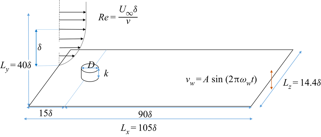
For convenience, the origin of the streamwise axis is placed at the location of the roughness element. The leading edge of the flat plate is not included since we only focus on the roughness-induced disturbance in this study. The computational domain and the definition of the problem are sketched in figure 1. The roughness element takes the form of a circular cylinder and its aspect ratio is  $D/k$, where
 $D$ is the diameter of the cylinder and
 $k$ is the height of the cylinder. Unless otherwise stated, the aspect ratio
 $D/k=1$ and
 $k=0.5\delta$. This form of roughness allows us to compare current results with rich works in the literature (Loiseau et al. Reference Loiseau, Cherubini, Robinet and Leriche2014; Bucci et al. Reference Bucci, Puckert, Andriano, Loiseau, Cherubini, Robinet and Rist2018; Puckert & Rist Reference Puckert and Rist2018). The geometric dimensions of the computational domain are
 $L_x=105\delta$,
 $L_y=20\delta$ and
 $L_z=14.4\delta$ in the streamwise, vertical and spanwise directions, respectively. The streamwise length is chosen to ensure that the flow structures downstream of the roughness element are fully developed. The spanwise size of the domain ensures that the roughness element behaves as an isolated one, in accordance with the study of Loiseau et al. (Reference Loiseau, Cherubini, Robinet and Leriche2014). The Blasius boundary-layer thickness at the location of roughness element is fixed at
 $\delta =1$ throughout this investigation, regardless of the Reynolds number. This is realised by moving the inlet plane further upstream when the Reynolds number is decreased, ensuring that the influence of the boundary-layer thickness is removed when the Reynolds number is varied.
A schematic diagram of the computation domain.

The Blasius velocity profile is implemented at the inlet using a Dirichlet velocity boundary condition. At the outlet, a Neumann boundary condition is applied on the velocity,  $\boldsymbol {\nabla }_{n}\boldsymbol {\cdot }\boldsymbol {u}=0$. At the far-field boundary
 $y=40\delta$, velocity conditions
 $\partial {u}/\partial {x}=0$,
 $v=-A\sin (\omega _w{t})$,
 $w=0$ are adopted. No-slip boundary condition is imposed on the flat plate and the surface of the roughness element. In the spanwise direction, periodic boundary conditions are used at
 $z=0$ and
 $z=L_z$.
The no-slip boundary condition on the surface of the roughness element is fulfilled using the IBM proposed by Goldstein, Handler & Sirovich (Reference Goldstein, Handler and Sirovich1993). The force exerted on the roughness by the fluid around it can be described by
 \begin{equation} \boldsymbol{F}=\sigma\int_{0}^{t}[\boldsymbol{u}(\boldsymbol{x}_s,\hat{t})-\boldsymbol{V}(\boldsymbol{x}_s,\hat{t})]\, \mathrm{d}\hat{t}+\beta[\boldsymbol{u}(\boldsymbol{x}_s,t)-\boldsymbol{V}(\boldsymbol{x}_s,t)], \end{equation}
where  $\boldsymbol {V}(\boldsymbol {x}_s,t)=(0,0,0)^{\rm T}$ is the desired velocity vector on the surface of the roughness element;
 $\boldsymbol {x}_s$ denotes the boundary points of the roughness element where the force is applied;
 $\boldsymbol {u}(\boldsymbol {x}_s,t)$ is the actual velocity at the boundary points during the simulation. Here,
 $\hat {t}$ is an integral variable from the initial time to the present time
 $t$;
 $\sigma$ and
 $\beta$ are negative constants, and are selected based on the viscous time scale
 $t_v=\nu /u^2_\tau$, where
 $u_{\tau }$ is friction velocity;
 $\sigma ^{-1/2}=0.45t_v$ and
 $\beta ^{-1}=0.2t_v$ are used in this study, as proposed by Forooghi et al. (Reference Forooghi, Stroh, Schlatter and Frohnapfel2018). The body force can be considered as a feedback control that suppresses the deviation of velocity at the fluid–solid boundary from the desired value. In implementation, the force is spread to the fluid mesh using the four-point Dirac function to obtain the body force
 $\boldsymbol {f}$ on the fluid (Peskin Reference Peskin2002)
 \begin{equation} \boldsymbol{f}=\int{\boldsymbol{F}\delta_D(\boldsymbol{x}-\boldsymbol{x}_s)\,\mathrm{d}s}, \end{equation}
where  $\delta _D$ is a Dirac function widely used in IBM (Peskin Reference Peskin2002). The present IBM implementation has been validated by another solver adapting a different algorithm (Deng, Mao & Xie Reference Deng, Mao and Xie2019) in the study of fluid and structure interactions.
Spatial discretisation of (2.1) is performed using a spectral element method (Karniadakis & Sherwin Reference Karniadakis and Sherwin2007). Each  $x$–
 $y$ plane is decomposed into 3915 elements, clustering around the wall. Each element is further decomposed into a
 $(P+1)(P+1)$ grid to perform Lagrange interpolation of order
 $P$. In this work,
 $P=7$ is adopted after a convergence study (Huang et al. Reference Huang, Xiao, Ren, Wang, Xi and Mao2021). In the spanwise direction, the flow variables are decomposed into 72 Fourier modes over the spanwise width of 14.4
 $\delta$.
3. Direct numerical simulations
In this section, we will analyse the wall-normal vibration-induced transition on a flat plate with a roughness element using DNS. First, a broad view showing the effect of vibration on boundary-layer flow in the presence of a roughness element is given in § 3.1. Then a parametric study is conducted in § 3.2 to further identify the effects of vibration magnitude, the Reynolds number and roughness diameter/height on transition. Finally, the instabilities leading to transition are discussed in § 3.3.
3.1. Vibration-induced transition
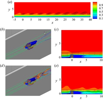
The flow under study consists of two key components: roughness and vibration. Equation (2.1) is solved under different conditions in order to gain understanding of their individual effects. Then they are combined to give a view of the joint effect. Solving (2.1) with  $\boldsymbol {f}=0$, we obtained the boundary-layer flow with vibration only and the result is shown in figure 2(a). The vertical vibration of the wall introduces a 2-D wavy disturbance to the flow, which is manifested as spanwise vorticity sheets. The vibration-induced disturbance in the absence of roughness is defined by the deviation of velocity from the Blasius velocity profile. On the other hand, boundary-layer flow with a cylinder roughness element only is obtained by setting the vibration-induced forcing terms to zero, as illustrated in figures 2(b) and 2(c). When impinging on the roughness element, the boundary-layer flow warps around the roughness and a horseshoe vortex is formed upstream of the cylinder. On the sides of the cylinder, the legs of the horseshoe vortex continue to travel downstream as a pair of counter-rotating vortices. Behind the roughness element a reverse flow region is created due to the blockage of the roughness. Downstream of the wake zone, the base flow without vibration is steady and no vortex shedding is observed at
 $\textit {Re}=700$. Figures 2(d) and 2(e) show the flow development with the combination of a surface roughness and vertical vibration. When the wall is vibrating in the wall-normal direction, the streamwise vorticity behind the roughness becomes much stronger and vortex shedding appears, indicating that the vibration-induced disturbance is amplified in the wake of the roughness element. We only show the flow structures and wakes under vibration with
 $(\omega _w,A)=(1.23,0.02)$, at which the difference in the flow development with and without roughness is prominent. The influence of vibration amplitude and frequency will be investigated in detail in §§ 3.2 and 3.3, respectively.
Influence of vibration on boundary-layer flow at  $\textit {Re}=700$ and
 $(A,\omega _w)=(0.02,1.23)$. (a) Boundary-layer flow on a vibrating plate, visualised by the contour of velocity, with contour lines of vibration-induced velocity fluctuation. (b) Visualisations of flow structures around the roughness element on a non-vibrating plate. Iso-surface coloured in blue is
 $u=0$, circling the reverse flow region. Iso-surfaces coloured in purple and orange are streamwise vorticity
 $\omega _x=\pm 1$. Streamlines around the cylinder are coloured by
 $u$. (c) Wake zone behind the roughness on a non-vibrating plate, visualised by contours of
 $u$. (d) Visualisations of flow structures around the roughness element on a vibrating plate. (e) Wake zone behind the roughness on a vibrating plate.

It is worth mentioning that, for a 2-D cylinder in a uniform flow, the critical Reynolds number (based on the local velocity and diameter of cylinder) for vortex shedding is approximately 47 (Provansal, Mathis & Boyer Reference Provansal, Mathis and Boyer1987). In the current study, both the boundary layer on the plate and the diving shear flow from the top of roughness alter the critical Reynolds number of von Kámán vortex shedding. Moreover, the horseshoe vortex developed at the corner of the cylinder and the ground plate can also significantly modify the vortex shedding (Okamoto & Sunabashiri Reference Okamoto and Sunabashiri1992). Consequently, there is no vortex shedding observed in figure 2(b) when the flat plate is non-vibrating even though the local Reynolds number is approximately 540.
3.2. Parametric study on effect of  $Re$ and $A$


Intuitively, bypass transition can be promoted by increasing the Reynolds number and the vibration magnitude. In this section, the joint effect of  $\textit {Re}$ and
 $A$ will be studied with the frequency of vibration fixed at 0.628, while the effect of
 $\omega _w$ will be addressed in § 3.3. Figure 3 shows the velocity streaks depicted by iso-surfaces of
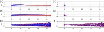
 $u_s$, i.e. the deviation of streamwise velocity from the Blasius velocity profile, on non-vibrating plates at different Reynolds numbers. As can be seen from figures 3(a) and 3(b), the CRP downstream of the roughness element generates three steady low-speed streaks. The central low-speed streak fades away quickly downstream. The two low-speed streaks on the flanks develop further downstream, and then decay when
 $\textit {Re}$ is small. Two high-speed streaks are initially generated between the three low-speed ones around the roughness, and they merge into one large streak further downstream with the central low-speed streak vanishing completely. When the Reynolds number is increased to
 $\textit {Re}=800$ (figure 3c, f), the flow becomes unstable, and thus the vorticity generated by the roughness is sustained. The amplitude of streaks continues to grow and eventually the streaks breakdown due to the generation of streamwise vorticity, which has been widely studied experimentally (Puckert & Rist Reference Puckert and Rist2018, Reference Puckert and Rist2019) and numerically (Loiseau et al. Reference Loiseau, Cherubini, Robinet and Leriche2014; von Deyn et al. Reference von Deyn, Forooghi, Frohnapfel, Schlatter, Hanifi and Henningson2020). The transition Reynolds number for the non-vibrating plate is approximately 800, below which the streamwise vorticity decays quickly downstream due to the viscous effect (figure 3d,e).
Iso-surfaces of  $u_s=\pm 0.1$ (a–c) and streamwise vorticity
 $\omega _x=\pm 0.5$ (d–f) in a non-vibrating plate flow, where
 $u_s$ is defined as the deviation of the streamwise velocity from the Blasius velocity profile; (a,d)
 $\textit {Re}=500$, (b,e)
 $\textit {Re}=700$ and (c, f)
 $\textit {Re}=800$.

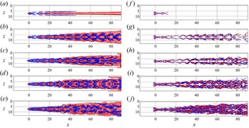
On the other hand, figure 4 presents the flow field downstream of the same roughness element as in figure 3, but with the flat plate vibrating vertically. At  $\textit {Re}=400$ (figure 4a, f), the streamwise vorticity decays under the strong viscous dissipation effect. As a result, the low-speed streaks still fade away even when the wall is vibrating. As
 $\textit {Re}$ increases to 500 (figure 4b,g), the vibration of the wall clearly enhances streamwise vorticity downstream of the roughness, which gives rise to stronger velocity streaks. The vibration brings about a zigzag pattern of the streamwise vorticity and the meandering of low-speed streaks can be observed. The transition Reynolds number is therefore reduced to approximately
 $400< Re_t<500$ due to the vibration of the wall. Further increasing the Reynolds number results in stronger streamwise vorticity and earlier breakdown of velocity streaks (figure 4c–j). Comparison of figures 3 and 4 clearly suggests that the vibration of the wall strengthens the roughness-induced disturbance and promotes the instability and breakdown of the streaks by enhancing the streamwise vorticity. The instability responsible for the amplification of streamwise vorticity by vibration will be explored later in this paper.
Iso-surfaces of  $u_s=\pm 0.1$ (a–e) and streamwise vorticity
 $\omega _x=\pm 0.5$ ( f–j) in a vibrating plate flow. The vibration amplitude and frequency are fixed at
 $(\omega _w, A)=(0.628, 0.02)$ in these cases; (a, f)
 $\textit {Re}=400$, (b,g)
 $\textit {Re}=500$, (c,h)
 $\textit {Re}=600$, (d,i)
 $\textit {Re}=700$ and (e,j)
 $\textit {Re}=800$.

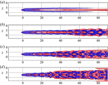
Figure 5 examines the effect of vibration amplitude on the flow development. The influence of vibration is insignificant at  $A= 0.0005$ (figure 5a). When
 $A$ is increased to 0.002 (figure 5b), the velocity streaks remain unchanged in the wake zone of the roughness. Downstream of the roughness wake, one can observe the meandering motion of low-speed streaks at
 $x\approx 20$. The velocity streaks on the flanks break into segments, forming a rhombus structure at
 $x>60$. As can be seen in figures 5(c) and 5(d), higher vibration amplitude promotes the instability and breakdown of the velocity streaks with large rhomboidal structures appearing more upstream. Especially at
 $A=0.02$, the instabilities of the low-speed streaks on the two sides occur almost in the immediate roughness wake (figure 5d). It is also worth noting that the flow pattern before the breakdown of streak remains the same regardless of the vibration amplitude, indicating the same instability mechanism at sufficiently strong vibrations (
 $A>0.0005$).
Iso-surfaces of  $u_s=\pm 0.1$ on a vibrating plate at different vibration amplitudes; (a)
 $A=0.0005$, (b)
 $A=0.002$, (c)
 $A=0.005$, (d)
 $A=0.02$. For these cases (
 $\textit {Re},\omega _w$) are fixed at (
 $700, 0.628$).

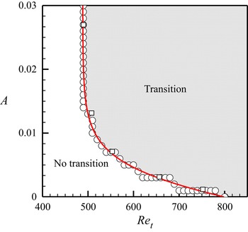
The dependence of the transition Reynolds number on the vibration amplitude is shown in figure 6. Unless otherwise stated, we use subscript  $t$ to denote the critical value above which the flow is transitional. For the non-vibrating case (
 $A=0$), the transition Reynolds number is approximately 800. The local Reynolds number based on local velocity at the position of roughness and height of
 $k$ is approximately 625, which falls within the transitional region in the diagram collected by von Doenhoff & Baslow (Reference von Doenhoff and Baslow1961) at
 $D/k=1$. Puckert & Rist (Reference Puckert and Rist2018) report a transition Reynolds number of about 860 when the inlet plane locates at
 $x_k=166.4$. The transition Reynolds number in the current study is close to their results. For the vibration cases, it can be seen that the transition Reynolds number gradually decreases as the vibration amplitude increases. The fitted curve is almost linear until
 $\textit {Re}=600$, after which it converges to a straight vertical line at
 $\textit {Re}=500$. In other words, a stronger (weaker) vibration is required to change the stability state of the flow when the Reynolds number is low (high). This trend is reasonable since the flow is more unstable at higher
 $\textit {Re}$ such that a small change of external forcing can make a significant difference. It can also be concluded that the absolute transition Reynolds number is 500, below which there is no transition regardless of the vibration amplitude. It can be seen that the joint effect of
 $\textit {Re}$ and
 $A$ on transition is insensitive to
 $\omega _w$ as long as it is within the effective range (figure 6, square points).
Variation of the transition Reynolds number with the vibration amplitude  $A$ at
 $\omega _w=0.628$ (circle symbols) and
 $\omega _w=0.91$ (square symbols). Symbols are simulation cases; red line is a fitted curve.

The above discussions show that, as long as the Reynolds number is in the range of  $500<\textit {Re}<800$,
 $Re$ and
 $A$ are coupled together to determine the transition state of the flow. For
 $\textit {Re}$ smaller than 500, transition does not occur regardless of the vibration amplitude, while for
 $\textit {Re}$ greater than 800, transition is triggered even without any vibration. The route to transition is similar when the vibration amplitude or Reynolds number is varied within this range of parameters, indicating the same instability mechanisms in these cases.
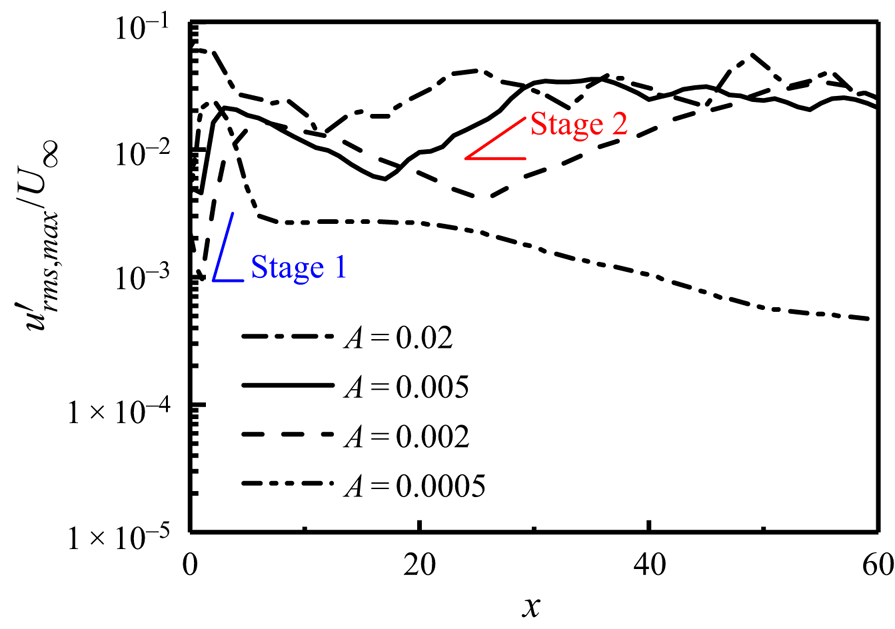
Figure 7 displays the streamwise variations of the strength of the disturbance under different vibration amplitudes. At small vibration amplitude  $A=0.0005$, the disturbance increases linearly in the immediate wake of the roughness, before decaying monotonically due to viscosity as it convects downstream. For larger
 $A$, the streamwise variations of the disturbance are completely different and can be grouped into two stages. The first stage appears in the immediate wake of roughness (
 $0< x<5$) similar as in the small amplitude case, whereas the second one is located further downstream and associated with the low-speed streak. It can also be seen that higher
 $A$ only moves the starting location of the second stage more upstream, but does not affect the peak value. The two growth stages are not only spatially separated, but also have different growth rates, suggesting that there are two different instability mechanisms supporting the two growths of disturbance. Identification and detailed investigation of the two instabilities will be presented in the next section.
Streamwise evolution of the maximum root mean square of streamwise velocity fluctuation  $u'_{{rms}}$ under different vibration amplitudes. The Reynolds number and vibration frequency are fixed at
 $(\textit {Re},\omega _w)=(700, 0.628)$ in these cases.

In addition to the baseline case (roughness diameter  $D=0.5\delta$ and height
 $k=0.5\delta$), we further investigate effects of roughness parameters. We focus on roughness smaller than the boundary-layer thickness, which is in line with most practical applications of this type of problem. Here,
 $D$ and
 $k$ are varied from
 $0.1\delta$ to
 $1.0\delta$ and
 $0.1\delta$ to
 $0.6\delta$, respectively. Such a parameter space covers a region wide enough to represent small roughness cases, allowing variations of the roughness aspect ratio (
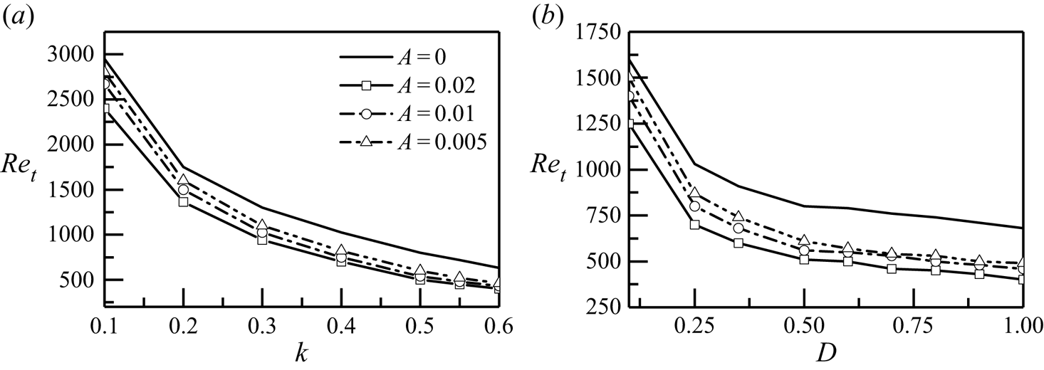
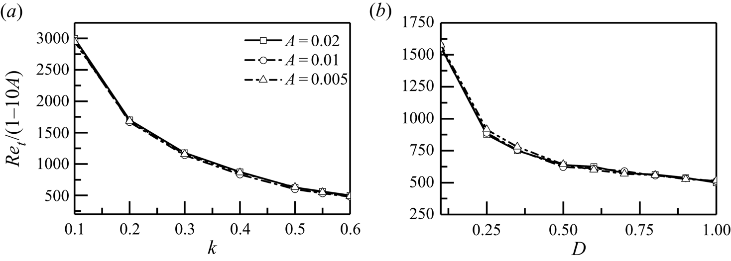
 $D/k$) ranging from 0.2 to 5. Figures 8(a) and 8(b) present the effect of
 $k$ and
 $D$ on the critical Reynolds number
 $Re_t$, respectively. Here,
 $Re_t$ decreases quickly with the increase of
 $k$ and it is not sensitive to the vibration amplitude when
 $k$ is large. More specifically, for
 $k>0.5$, vibration with
 $A=0.005$ significantly reduces the transition Reynolds number, and the effect of vibration saturates when we further increase
 $A$. On the other hand,
 $Re_t$ decreases when increasing
 $D$; and the descending trend becomes mild when
 $D$ is above
 $0.5$. Scaling
 $Re_{{t}}$ by
 $(1-10A)$, it is found that among all the parameters studied, the effect of the vibration on the critical
 $\textit {Re}$ can be unified, as displayed in figure 9. In the following study, we will focus on
 $A=0.02$ and
 $\textit {Re}=700$. This Reynolds number is selected such that the flow is still globally stable when the wall is non-vibrating (as shown in figures 3b and 3e).
Variations of the transition Reynolds number with the roughness size of (a) fixed  $D=0.5$ and varying
 $k$, and (b) fixed
 $k=0.5$ and varying
 $D$.

Variations of scaled  $Re_{t}$ with the roughness size of (a) fixed
 $D=0.5$ and varying
 $k$, and (b) fixed
 $k=0.5$ and varying
 $D$.

3.3. The instabilities leading to transition
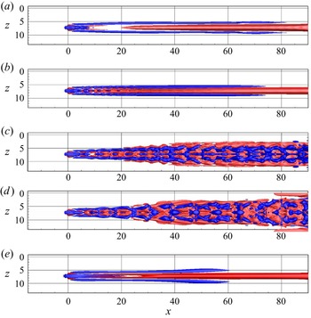
The evolution of disturbance shown in § 3.2 indicates that can be two instabilities contributing to the transition: one in the immediate wake zone, and the other further downstream related to the velocity streaks on the flanks. Figure 10 shows the velocity streaks on the vibrating plate with different vibration frequencies to verify this observation. As mentioned previously, the vibration frequency is decoupled from  $Re$ and
 $A$ (figure 6) as it is not related to the energy balance (i.e. viscosity dissipation or momentum input) of the flow. However, as shown in figure 10, the stability of the streaks is significantly affected by the frequency of vibration. At
 $\omega _w=2.09$ (figure 10a), one can observe the deformation of the central negative velocity streak in the wake zone. Whilst further downstream, the streaks appear to be steady. The effect of vibration is extended to
 $x\approx 20$ when the vibration frequency is reduced to
 $\omega _w=1.40$ and the deformation of streaks in the centre as well as on the flanks are visible at this frequency (figure 10b). However, the instability here does not lead to streak deformations that are strong enough to breakdown, and the disturbances eventually decay further downstream. Bypass transition is triggered through the breakdown of streaks as
 $\omega _w$ decreases, as shown in figures 10(c) and 10(d). The meandering motion of streaks appears as early as
 $x=5$. Within the effective vibration frequency range, it is clear that smaller
 $\omega _w$ leads to earlier breakdown locations. It can also be noted that the vibration frequency is inversely proportional to the streamwise wavelength of the deformed streaks. Therefore, when
 $\omega _w$ approaches zero (e.g. 0.05 as shown in figure 10e), the streaks simply decay downstream before any deformation appears.
Iso-surfaces of  $u_s=\pm 0.1$ on a vibrating plate with
 $(\textit {Re},A)=(700,0.02)$ and (a)
 $\omega _w=2.09$, (b)
 $\omega _w=1.40$, (c)
 $\omega _w=0.91$, (d)
 $\omega _w=0.628$, (e)
 $\omega _w=0.05$.

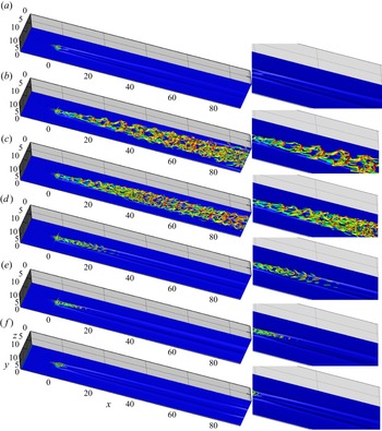
According to Acarlar & Smith (Reference Acarlar and Smith1987), the central hairpins shed from the roughness element immersed in the boundary layer are correlated to the shear layer wrapped around the roughness. Other researchers also observed the shedding of hairpins from roughness at larger  $\textit {Re}$ (Loiseau et al. Reference Loiseau, Cherubini, Robinet and Leriche2014) or higher roughness element (Bucci et al. Reference Bucci, Puckert, Andriano, Loiseau, Cherubini, Robinet and Rist2018), and they attribute the shedding of central hairpins to the instability of the 3-D shear layer detached from the roughness. In our study, there are no central hairpins shed from the roughness when the flat plate is non-vibrating (figure 3d), as the Reynolds number/roughness height is smaller than those in the literature. The vortical structures developed downstream of the roughness when the flat plate is vibrating at various frequencies are presented in figure 11. At
 $\omega _w=0.05$, as the period of vibration is relatively long, the flow is similar to that on a non-vibration plate and no hairpin vortex is captured downstream of the roughness (figure 11a). Central hairpin vortices are shed from the roughness at vibration frequencies ranging from 0.628 to 2.09, as shown in figure 11(b–e). As mentioned before, the vibration frequency is inversely proportional to the streamwise wavelength of the hairpins and higher
 $\omega _w$ leads to smaller structures. Above
 $\omega _w=2.09$, the hairpins are formed and then decay downstream, and at
 $\omega _w=3.2$ (figure 11f) there is almost no central hairpin shedding from the roughness.
Vortical structures on a vibrating plate with different vibration frequencies at  $(\textit {Re},A)=(700,0.02)$, with iso-surface of
 $u=0.2$ as the background; (a)
 $\omega _w=0.05$, (b)
 $\omega _w=0.628$, (c)
 $\omega _w=0.91$, (d)
 $\omega _w=1.40$, (e)
 $\omega _w=2.09$, ( f)
 $\omega _w=3.20$. Vortical structures are depicted by iso-surface of
 $\lambda _2=-0.05$. Right column presents the corresponding zoomed in view of vortical structures downstream of the roughness.

The mechanism for the generation of hairpin vortices in a shear flow has been revealed by Cohen, Karp & Mehta (Reference Cohen, Karp and Mehta2014), who found that a pair of counter-rotating streamwise vortices and a 2-D streamwise wavy spanwise vortex sheet in the shear flow are inherently unstable and evolve into a packet of hairpin vortices. They suggested that such instability is due to the inviscid inflectional instability of the base shear. In our study, the combination of vibration-induced spanwise vortex sheet and the roughness-induced CRP is similar to the model proposed by Cohen et al. (Reference Cohen, Karp and Mehta2014). Based on above DNS results, it can be concluded that the instability of the wall-normal shear layer in the wake zone is activated to amplify the vibration-induced disturbance, causing the undulation of the CRP and then giving rise to a packet of central hairpin vortices downstream of the roughness. Since the shear layer in the wake is highly unstable, it can amplify disturbance in a wide range of frequencies. Therefore, the shedding of central hairpins is observed at the vibration frequency ranging from 0.628 to 2.09. Outside this range, no hairpin vortices are produced, as seen in figures 11(a) and 11( f). For brevity, it is termed the wake mode instability in the following discussion. As the wake mode instability is closely related to the shear layer at top of the roughness, the velocity fluctuation is strongest at the location of roughness and initially decays when the shear stress is dissipated by viscosity, which is evident in figure 7.
When the vibration frequency is below 1.4, streamwise vorticities are developed on the low-speed streaks on both sides and the vorticity twists the low-speed streak to meander (figure 11d). At smaller vibration frequencies (figure 11b,c), the instability of the streaks on the sides is strong enough that new hairpin vortices are formed on the low-speed streaks. The interaction of the central and side hairpins results in the burst out of smaller vortex structures in the flow. As reported by many researchers (Asai, Minagawa & Nishioka Reference Asai, Minagawa and Nishioka2002; Chernoray et al. Reference Chernoray, Kozlov, Lofdahl and Chun2006), the instability of streaks, both varicose and sinuous types, can induce the formation of hairpin vortices. More recently, Wang, Huang & Xu (Reference Wang, Huang and Xu2015) found that the sinuous instability of streaks can lead to an alternatively aligned streamwise vorticity with opposite sign along the streaks, which then gives birth to hairpin vortices via stretching and turning of the positive and negative streamwise vorticity. In experiments, Konishi & Asai (Reference Konishi and Asai2010) found that the subharmonic sinuous instability of a pair of low-speed streaks leads to the connection of streamwise vortices, resulting in the formation of the head of hairpin. Similarly, Li, Dong & Lu (Reference Li, Dong and Lu2014) found that the spanwise-inclined and upward-tilted streamwise vortices induced from subharmonic sinuous instability of streaks form an ‘X-like’ vortical structure, which develops into a  $\varLambda$ vortex and then a hairpin vortex. The generation of hairpins downstream of the roughness wake in our study is in agreement with their results. The sinuous instability of the streaks produces zigzag streamwise vorticity with alternative signs (figure 4h), which evolves into hairpins on the sides. The subharmonic sinuous instability of a pair of streaks connects the streamwise vorticity on two sides to form new central hairpins further downstream (figure 11b). In other words, the new hairpins on the sides are inherently different from the central hairpins in the immediate wake of the roughness. They are produced by the instabilities of the streaks instead of instability of the shear layer wrapped around the roughness. Since the instability is related to the velocity streak, it is termed the streak mode instability in the following discussion.
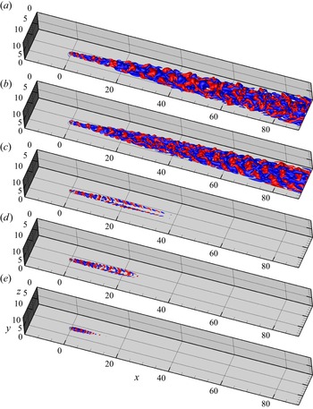
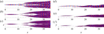
The evolution of the disturbance further shows the wake mode and streak mode instabilities in the flow. The streamwise development of the wall-normal velocity fluctuations from DNS is displayed in figure 12. In the wake zone ( $0< x<10$), the perturbations cluster around the centre and exhibit a symmetric pattern. Similar to before, the streamwise wavelength of the perturbation in the wake zone varies with the vibration frequency. For
 $\omega _w<1.4$, perturbations also develop from the streaks on two sides downstream of the wake zone (figure 12a,b). The perturbations with opposite sign overlap with each other in the spanwise direction, producing more disturbances around the velocity streaks. The streak mode instability is sustained and amplified at these cases. For a vibration frequency between 1.4 and 1.7, the perturbations develop downstream of the wake zone, and they also overlap with each other in the spanwise direction (figure 12c,d). However, the perturbations on two sides decay further downstream, implying that the streak mode instability is weak and vanishes downstream. For high vibration frequency (
 $\omega _w=2.09$), the streak mode instability is not triggered, leading to monotonic decay of disturbance downstream of the roughness (figure 12e).
Iso-surfaces of wall-normal velocity fluctuation  $\pm 0.05$ at different frequencies; (a)
 $\omega _w=0.628$, (b)
 $\omega _w=0.91$, (c)
 $\omega _w=1.40$, (d)
 $\omega _w=1.70$, (e)
 $\omega _w=2.09$.

4. The wake mode and streak mode instabilities
In order to confirm the instabilities observed in DNS in the previous section, Floquet analyses and DMD are performed to further investigate the stability of the flow in this section.
4.1. Linear Floquet analysis
When the Reynolds number is low enough ( $Re<800$), there is no recirculation zone behind the roughness element and the flow is globally stable. However, the flow is still capable of amplifying the disturbance transiently. In other words, the flow is convectively unstable, supporting the spatial growth of the perturbations. The convective instability of the flow is studied by linear Floquet analysis in
 $y$–
 $z$ planes The disturbance to the periodic base flow
 $\boldsymbol {q}'_f=(\boldsymbol {u}'_f,p'_f)$ satisfies the linearised equations
 \begin{equation} \partial _{t} \boldsymbol{u}'_f+\boldsymbol{u}_b\boldsymbol{\cdot}\boldsymbol{\nabla}\boldsymbol{u}'_f+\boldsymbol{u}'_f\boldsymbol{\cdot} \boldsymbol{\nabla}\boldsymbol{u}_b+\boldsymbol{\nabla} p'_f-\textit{Re}^{{-}1}\nabla^{2}\boldsymbol{u}'_f+ \boldsymbol{v}_{w}\boldsymbol{\cdot} \boldsymbol{\nabla}\boldsymbol{u}'_f=0, \boldsymbol{\nabla}\boldsymbol{\cdot} \boldsymbol{u}'_f=0,\end{equation}
where  $\boldsymbol {u}_b$ is phase-averaged base flow with frequency
 $\omega _w$ at
 $y$–
 $z$ planes from DNS. Invoking a normal mode assumption in the streamwise direction, one obtains
 \begin{equation} \boldsymbol{q}'_f(t=2{\rm \pi}/\omega_w)=\hat{\boldsymbol{q}}'_{f}(t=0) \exp({\textrm{i}\alpha{x}+\gamma{2{\rm \pi}/\omega_w}}), \end{equation}
where  $\alpha$ is the streamwise wavenumber of the instability,
 $\gamma$ is the growth per time unit integrated over one period and the time interval is set to be aligned with the period of the base flow, i.e.
 $2{\rm \pi} /\omega _w$. The instability problem is converted to an eigen problem when substituting this ansatz into (4.1)
 \begin{equation} \gamma\boldsymbol{u}'_f=\mathcal{L}\boldsymbol{u}'_f, \end{equation}
where  $\mathcal {L}$ is a linear operator describing the linear stability of the underlying periodic base flow
 $\boldsymbol {u}_b$. The solution to this eigen problem is obtained by implementing the Arnoldi scheme (Barkley, Blackburn & Sherwin Reference Barkley, Blackburn and Sherwin2008).
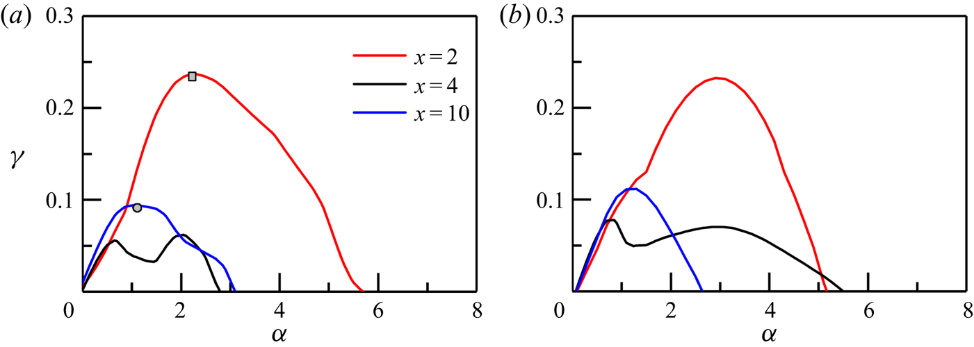
Figure 13 shows the growth rate  $\gamma$ against perturbation wavenumber at different streamwise locations. As can be seen in figure 13(a), the two instabilities observed before belong to different curves in the eigen space. The instability growth for the wake mode (
 $x=2$) reaches its maximum at
 $\alpha =2.2$, whereas the streak mode (
 $x=10$) peaks at a lower wavenumber
 $\alpha =1.2$. The wake of the cylinder is sensitive to the disturbance in a wide range of streamwise wavenumber
 $\alpha$ values. The condition for the K–H instability is
 $0<\alpha {h_s}<1.2785$, where
 $\alpha$ is wavenumber and
 $h_s$ is the thickness of the shear layer (Chandrasekhar Reference Chandrasekhar1961). In the current study, the shear layer thickness on top of the roughness is approximately 0.3 and hence the unstable region for
 $\alpha$ is
 $0<\alpha <4.27$, which matches with the result shown in figure 13(a). Thus it further confirms previous DNS findings that the wake mode instability is related to the wall-normal shear on top of the roughness. The wavenumber of streak instabilities reported by other researchers is in the range of 0.5–1.2 (Hack & Zaki Reference Hack and Zaki2014b; Wang, Mao & Zaki Reference Wang, Mao and Zaki2019), which is also in agreement with the current results. The apparent variation of wavenumber also implies different types of instability mechanisms. The growth rate at
 $x=4$ is also plotted in figure 13 to illustrate that the identified differences between the wake and streak modes are not due to the streamwise variations of the base flow. Moving the base flow from
 $x=2$ to
 $x=4$ results in an obvious decrease of the growth rate, but the peak wavenumbers at these two locations are not changed. Another peak is presented at
 $\alpha \approx 0.8$, which implies the emergence of another instability mode. More importantly, the growth rate at
 $x=10$ is higher than that at
 $x=4$, indicating that the shift of growth rate curve from
 $x=2$ to
 $x=10$ cannot be attributed to the deformation of a single instability mode affected by the variations of base flow; as the latter one is expected to present a continuous and monotonic change of growth rate. The results for a higher-frequency vibrating case with
 $\omega _w=0.91$ are displayed in figure 13(b), where two branches of growth rates can also be seen. It is worth noting that the wavenumber of the wake mode increases with the vibration frequency (more details are shown in figure 15).
Instability growth rate at different streamwise locations for  $(\textit {Re}, A)=(700, 0.02)$ and (a)
 $\omega _w=0.628$ (b)
 $\omega _w=0.91$.

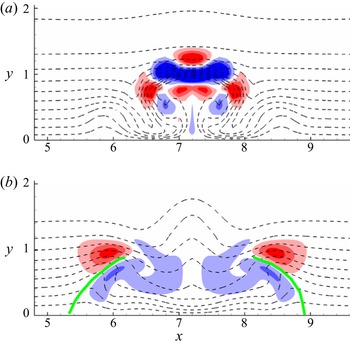
The two instability modes can be further distinguished by their structures, as shown in figure 14. The dashed line represents the time-averaged base flow. In figure 14(a), the wake mode is concentrated in the shear in the wall-normal direction in the centre, which indicates that the wake mode is related to the shear layer on top of the roughness. The green lines in figure 14(b) mark the centre of low-speed streaks on two sides. The two streak modes develop simultaneously around the low-speed streaks and present an asymmetric pattern with respect to each streak, suggesting that the streak mode instability is of sinuous type due to the spanwise shear of the flow.


The variations of the base flow in the streamwise direction play a key role in the evolution of instability of the flow. However, from the above observations, it is clear that the wake mode and streak mode instabilities have completely different mechanisms and thus should not be considered as the same. Variations of base flow in the streamwise direction supporting different instability modes were reported in other studies. For example, the research on jet turbulence by Schmidt et al. (Reference Schmidt, Towne, Rigas, Colonius and Bres2018) showed that the K–H mechanism dominates the instability of the very-near-nozzle shear layer, whereas the instability downstream of the jet core region is associated with the Orr mechanism.
Figure 15 presents a quantitative comparison of the instability wavenumber from the Floquet stability analyses and the DNS. For the wake mode instability,  $\alpha$ from the Floquet analyses is almost linearly proportional to the vibration frequency, which is confirmed by the DNS results. The variation of the streak mode instability wavenumber is not as apparent as that of the wake mode. The wavenumber slightly increases as the vibration frequency increases. Above a critical value of approximately
 $\omega _w=1.4$, the wavenumber of the streak mode instability drops to approximately 0.96, which is close to the value when the plate is non-vibrating (dashed-dotted line in figure 15). At frequency
 $\omega _w>1.4$, a weak streak instability is obtained from Floquet analyses which neglect the streamwise decay of the streaks, but this instability is not observed in DNS perhaps because the growth is too small to develop into secondary structures before the streaks decay.
Variation of the wake mode and streak mode instability wavenumber with vibration frequency.  $\alpha$ is the wavenumber that maximises the local growth rate at
 $x=2$ and
 $x=10$ from the Floquet analysis. In DNS,
 $\alpha$ is measured by evaluating the dominant wavenumber of the wall-normal velocity fluctuation in the wake zone (
 $1< x<8$) and downstream of the wake zone (
 $8< x<20$). The dashed-dotted line represents the streak mode wavenumber when the plate is non-vibrating.

4.2. Dynamic mode decomposition
DMD are performed to further investigate the 3-D dominant modes in the studied boundary-layer flow. Ever since its introduction by Schmid (Reference Schmid2010), DMD has been widely used in the analysis of flow dynamics (Hua et al. Reference Hua, Gunaratne, Talley, Gord and Roy2016; Towne, Schmidt & Colonius Reference Towne, Schmidt and Colonius2018). In current study, 100 snapshots are collected for each vibration period and a total number of snapshots  $n=400$ are used to perform DMD. Details of the implementation can be found in Schmid (Reference Schmid2010).
Figure 16 shows the eigenvectors from the DMD analysis of a representative case where both wake and streak instabilities are activated. It is clear that two distinct modes exist: the first one has a string of structures and is located in the centre roughness wake zone, while the second is seen further downstream with two separated strings developing simultaneously around the streaks on each side. The side view confirms that the wake mode is localised at the shear layer on the top of the roughness, whereas the streak mode originates from the bottom of the boundary layer. In addition to the distribution of the modes, their patterns are also different. The wake mode is normal to the spanwise coordinate with alternating signs in the streamwise direction, whereas the streak mode is aligned with respect to the spanwise shear on the two sides. Both of them support that there are two distinct instability modes in the flow. It should be noted that the two modes are found in the same DMD eigenvector because they are modulated by the vibration of the plate and thus have the same frequency.
Three representative dynamic modes with eigenvalue (a,d)  $(0.993+0.123i)$, (b,e)
 $(0.983+0.184i)$ and (c, f)
 $(0.969+0.245i)$ corresponding to the dominant ones in the spectrum from DMD analyses with
 $(A, Re, \omega _w)=(0.02, 700, 0.628)$. The left and right plots show the top and side views, respectively.

Loiseau et al. (Reference Loiseau, Cherubini, Robinet and Leriche2014) identified two kinds of instability in the downstream region of roughness-induced bypass transition in a boundary-layer flow: the varicose mode and the sinuous mode. The sinuous mode is related to von Kármán instability, whereas the varicose mode is similar to the instability reported by Acarlar & Smith (Reference Acarlar and Smith1987), which is related to the shear layer separated from the roughness element. The wake mode instability activated by the vibration in our study is similar to the varicose mode instability identified by Loiseau et al. (Reference Loiseau, Cherubini, Robinet and Leriche2014). As reported by Bucci et al. (Reference Bucci, Puckert, Andriano, Loiseau, Cherubini, Robinet and Rist2018), the varicose mode instability is highly sensitive to external forcing so that at sub-critical Reynolds number, the quasi-resonance of the least stable varicose mode with external disturbance at the same frequency can lead to the hairpin vortex shedding in experiments. However, the height of roughness in our study is smaller than that used by Bucci et al. (Reference Bucci, Puckert, Andriano, Loiseau, Cherubini, Robinet and Rist2018), which makes the flow more stable and no isolated varicose mode is found. The instability of the shear layer is activated by vibration-induced disturbance in a wide range of frequencies in current study, leading to the formation of a packet of hairpin vortices immediately after the roughness. The streak mode instability is fed on the streamwise vorticity legs of the hairpin vortex. A comparison of the transition scenarios for the non-vibrating and vibrating cases is shown in figure 17 at  $\textit {Re}=900$, at which bypass transition is triggered by roughness on the non-vibrating flat plate as seen in figure 17(a). In the laminar region, the shear layer in the wake zone is inherently unstable at this Reynolds number, leading to the formation of hairpin vortices downstream of the roughness. In the transitional region, the velocity streaks become unstable and more hairpin vortices are produced. The half-angle of the turbulent wedge developing downstream is approximately
 $5.6^{\circ }$ on the non-vibrating plate. On the other hand, when the plate is vibrating, the wake mode instability is apparently enhanced, leading to stronger and denser hairpins shedding from the roughness. More importantly, the vibration enhances the streamwise vorticity on both sides of the central hairpin legs, as shown at
 $x\approx 10$ in figure 17(b). The stronger streamwise vorticity advances the instability of the low-speed streak, giving rise to hairpins on two sides. The earlier interaction of the hairpin vortices promotes bypass transition on the vibrating plate. The half-angle of the turbulent wedge developing downstream is smaller in the vibrating case, which is approximately
 $4.5^\circ$.
Bypass transition of boundary-layer flow on vibrating and non-vibrating flat plates. Iso-surface of  $\lambda _2=-0.05$ is presented, with iso-surface of
 $u=0.2$ as the background; (a)
 $(\textit {Re}, A, \omega _w)=(900, 0, 0)$ and (b)
 $(\textit {Re}, A, \omega _w)=(900, 0.02, 0.628)$.

5. Generation of hairpin vortices
As previously observed, the instabilities eventually evolve into hairpins and their interaction causes more hairpins and the transition. The formation of hairpin vortices is key to understanding the bypass transition process.
A hairpin vortex is composed of two counter-rotating streamwise vorticity legs and an arch like head containing both the streamwise and transverse vorticity (Acarlar & Smith Reference Acarlar and Smith1987). Since hairpin is predominantly streamwise vortices, we examine the production terms of the streamwise vorticity  $\omega _x$ which is governed by
 \begin{equation} \frac{\mathrm{D}\omega_x}{\mathrm{D}t}=\underbrace{\omega_x \frac{\partial{u}}{\partial{x}}}_{\text{vorticity stretching}}+\underbrace{\omega_y\frac{\partial{u}}{\partial{y}}+\omega_z\frac{\partial{u}}{ \partial{z}}}_{\text{vorticity tilting}}+\textit{Re}^{{-}1}\nabla^{2}\omega_x, \end{equation}
where  $\omega _y$ and
 $\omega _z$ are wall-normal and spanwise vorticity, respectively. The first two terms on the right-hand side are the production terms of
 $\omega _x$, owing to vorticity stretching and tilting (Hack & Zaki Reference Hack and Zaki2014b), and the last term is the viscosity dissipation term. The streamwise velocity and vorticity can be decomposed into
 $$\begin{gather} u=U+u', \end{gather}$$
 $$\begin{gather}\omega_x=\varOmega_x+\omega_x', \end{gather}$$
where  $U$ and
 $\varOmega _x$ are the velocity and streamwise vorticity of the base flow when the wall is non-vibrating, and
 $u'$ and
 $\omega _x'$ are the corresponding fluctuations induced by the vibration of the wall.
Substituting (5.2) and (5.3) into the stretching term in (5.1), it becomes
 \begin{equation} \omega_x\frac{\partial{u}}{\partial{x}}=\varOmega_x\frac{\partial{U}}{\partial{x}}+\varOmega_x\frac{\partial{u'}}{\partial{x}}+\omega_x'\frac{\partial{U}}{\partial{x}}+\omega_x'\frac{\partial{u'}}{\partial{x}}. \end{equation}
Similarly, the tilting terms are
 $$\begin{gather} \omega_y\frac{\partial{u}}{\partial{y}}=\varOmega_y\frac{\partial{U}}{\partial{y}}+\varOmega_y\frac{\partial{u'}}{\partial{y}}+\omega_y'\frac{\partial{U}}{\partial{y}}+\omega_y'\frac{\partial{u'}}{\partial{y}}, \end{gather}$$
 $$\begin{gather}\omega_z\frac{\partial{u}}{\partial{z}}=\varOmega_z\frac{\partial{U}}{\partial{z}}+\varOmega_z\frac{\partial{u'}}{\partial{z}}+\omega_z'\frac{\partial{U}}{\partial{z}}+\omega_z'\frac{\partial{u'}}{\partial{z}}. \end{gather}$$
The last three terms in (5.4)–(5.6) are introduced by the vibration of the wall. The stretching and tilting terms are integrated separately over a control volume to identify their contributions to the production of  $\omega _x$. The magnitude of
 $\omega _x$ is intensified only if the sign of stretching (tilting) terms matches that of local
 $\omega _x$. Therefore, the net forcing that leads to an increase of
 $\omega _x$ within the volume can be defined as
 $$\begin{gather} P_s=\int_{CV}\frac{\omega_x}{|\omega_x|}\left(\underbrace{\varOmega_x\frac{\partial{U}}{\partial{x}}}_\text{1}+\underbrace{\varOmega_x\frac{\partial{u'}}{\partial{x}}}_\text{2}+\underbrace{\omega_x'\frac{\partial{U}}{\partial{x}}}_\text{3}+ \underbrace{\omega_x'\frac{\partial{u'}}{\partial{x}}}_\text{4}\right)\mathrm{d}V, \end{gather}$$
 $$\begin{gather}P_{ty}=\int_{CV}\frac{\omega_x}{|\omega_x|}\left(\underbrace{\varOmega_y\frac{\partial{U}}{\partial{y}}}_\text{1}+\underbrace{\varOmega_y\frac{\partial{u'}}{\partial{y}}}_\text{2}+\underbrace{\omega_y'\frac{\partial{U}}{\partial{y}}}_\text{3}+\underbrace{\omega_y'\frac{\partial{u'}}{\partial{y}}}_\text{4}\right) \mathrm{d}V, \end{gather}$$
 $$\begin{gather}P_{tz}=\int_{CV}\frac{\omega_x}{|\omega_x|}\left(\underbrace{\varOmega_z\frac{\partial{U}}{\partial{z}}}_\text{1}+\underbrace{\varOmega_z\frac{\partial{u'}}{\partial{z}}}_\text{2}+\underbrace{\omega_z'\frac{\partial{U}}{\partial{z}}}_\text{3}+\underbrace{\omega_z'\frac{\partial{u'}}{\partial{z}}}_\text{4}\right) \mathrm{d}V, \end{gather}$$
where  $P_s$,
 $P_{ty}$ and
 $P_{tz}$ are the integrated net production terms of streamwise vorticity from streamwise stretching, wall-normal tilting and spanwise tilting, respectively.
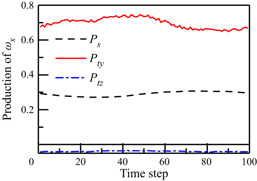
Figure 18 shows the integral of the production terms described above. The wall-normal tilting term contributes approximately 70 % of the total production of  $\omega _x$, whereas the streamwise stretching term accounts for approximately 30 %. In the study of streak instabilities by Hack & Zaki (Reference Hack and Zaki2014b), they also reported that the wall-normal tilting contributes approximately 70 % of the total production of
 $\omega _x$. It is noted that the spanwise tilting term has a negative effect on the generation of
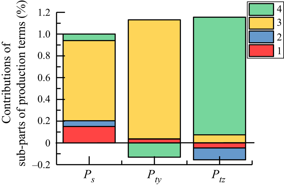
 $\omega _x$, indicating that the spanwise vorticity disturbance induced by vibration is not a direct source of the streamwise vorticity in the flow field. The mean contributions of different sub-parts of
 $P_s$,
 $P_{ty}$ and
 $P_{tz}$ are illustrated in figure 19. The relative importance of the stretching and tilting of the vorticity disturbance by the base flow is clear for
 $P_s$ and
 $P_{ty}$. Considering the contributions of
 $P_{ty}$ and
 $P_s$ to the total production of
 $\omega _x$, one can conclude that the tilting of
 $\omega _y'$ by the wall-normal shear of base flow is the major source for
 $\omega _x$, followed by the stretching of
 $\omega _x'$ by the streamwise velocity gradient of the base flow. Finally, the negative contribution of the spanwise tilting term stems from the nonlinear tilting effect of the disturbance field.
Integrated streamwise vorticity production terms  $P_s$,
 $P_{ty}$ and
 $P_{tz}$.

Mean contributions of different sub-parts of  $P_s$,
 $P_{ty}$ and
 $P_{tz}$. Sub-part 1 represents the stretching/tilting of the base-flow vorticity by the base-flow velocity gradients. Sub-part 2 represents the stretching/tilting of the base-flow vorticity by the disturbance velocity gradients. Sub-part 3 represents the stretching/tilting of the disturbance vorticity by the base-flow velocity gradients. Sub-part 4 represents the stretching/tilting of the disturbance vorticity by the disturbance velocity gradients.

6. Conclusion
Vibration-induced transition over a flat plate with a roughness element is studied by means of DNS. The vertical vibration of the flat plate introduces a 2-D wavy disturbance to the boundary-layer flow in the absence of roughness elements. When there is a cylinder roughness submerged in the boundary-layer flow, the shear layer detached from the roughness is destabilised by the vibration of the flat plate.
The boundary layer warps around the roughness element and a pair of counter-rotating streamwise vortices is formed downstream of the roughness, which leads to the formation of a central low-speed streak surrounded by two low-speed streaks on the sides. Both the Reynolds number and vibration amplitude affect the instability of the velocity streaks. For non-vibrating cases, the velocity streaks initially grow and then decay when the Reynolds number is below 800. This transition Reynolds number is significantly reduced to approximately 500 when the plate is vibrating with a frequency  $\omega _w<1.4$. Smaller Reynolds number requires a stronger vibration to activate transition in the flow and the transition Reynolds number–vibration magnitude line is collected. Investigations on roughness elements with
 $D=0.1\delta \textrm { to } 1.0\delta$ and
 $k=0.1\delta \textrm { to } 0.6\delta$ show that the critical Reynolds number at different vibration amplitudes
 $A$ can be unified by a scaling law of
 $(1-10A)$.
There are two different instabilities in roughness-induced transition over the vertically vibrating flat plate: the wake mode instability and streak mode instability. The effects of vibration frequency on these two modes of instability are investigated in detail. The former instability occurs in the immediate roughness wake and is general, appearing at almost all the parameters studied when there is vibration-induced disturbance. The wake mode instability results in the shedding of central hairpin vortices. The wavelength of the hairpin vortices depends on the frequency of vibration, such that at  $\omega _w$ above 3.2 or below 0.05, no hairpin vortices are shed from the roughness. This observation is in accordance with the investigation by De Tullio et al. (Reference De Tullio, Paredes, Sandham and Theofilis2013), who found that the roughness wake is highly unstable and capable to amplify forcing in a wide range of frequencies. The generation of central hairpins is attributed to the amplification of vibration-induced disturbance by the wall-normal shear layer in the roughness wake, which leads to the modulation of counter-rotating streamwise vortices behind the roughness element and then the production of hairpin vortices (Cohen et al. Reference Cohen, Karp and Mehta2014). The streak mode instability is sensitive to the vibration frequency of the flat plate, which is activated when the vibration frequency is between 0.628 and 1.4. The meandering of velocity streaks on the sides leads to the alternatively aligned streamwise vorticity with opposite sign, which then results in the generation of hairpins on the sides.
Linear Floquet stability analyses are performed using the time-periodic flow field from DNS as the base profile to further examine the instabilities. The two modes belong to different curves in the eigen space. The wake mode instability reaches its maximum growth rate at  $\alpha =2.2$, whereas the streak mode peaks at
 $\alpha =1.2$. The wake mode instability is localised within the wall-normal shear layer detached from the roughness. The streak mode instability, developing around the low-speed velocity streaks on the sides, appears further downstream and presents an asymmetric pattern with respect to the streak centre. Results from DMD further confirm that the two instability modes are spatially separated. The wake mode is normal to the spanwise coordinate with alternating signs in the streamwise direction. On the other hand, the streak mode originates from the bottom of the boundary layer and is aligned with respect to the spanwise shear on the two sides.
Finally, the generation of hairpin vortices is analysed by the production terms of streamwise vorticity. The wall-normal tilting term accounts for approximately 70 % of the generation of streamwise vorticity, whereas the streamwise stretching term is responsible for the other 30 % for the case studied. The spanwise tilting term itself does not contribute to the increase of streamwise vorticity when the plate is vibrating, indicating that the spanwise disturbance produced by the vertical vibration is not the direct reason for the increase of streamwise vorticity. Comparison of different sub-parts of the production terms shows that the amplification of disturbance by the base-flow shear dominates the production of streamwise vorticity.
Funding
We would like to acknowledge the financial support from National Natural Science Foundation of China (Grant Nos 52176044 and 92152109), and from the Key Research and Development Program of Shaanxi in China (Program No. 2018KW-017). Face-to-Face communication and collaboration of the authors are funded by the European Union's Horizon 2020 research and innovation programme under the Marie Skłodowska-Curie grant agreement No 777717.
Declaration of interests
The authors report no conflict of interest.