2.1 Problem formulation and numerical strategy

As in SC97, the flow in question is a fully turbulent incompressible ZPG boundary layer over a flat no-slip surface, subjected to first adverse then favourable mean streamwise pressure gradients. The pressure gradients are induced by a transpiration profile $V_{top}(x)$ through a virtual parallel plane offset a fixed distance $Y$ from the no-slip surface. Instantaneous realisations of off-the-wall and near-wall turbulence structures for one of the cases are illustrated in figure 1. Corresponding mean-flow contours and streamlines are shown in figure 2.

Figure 2.

Contours of mean streamlines and (a) streamwise velocity $\overline{u}$ and (b) spanwise vorticity $\overline{\unicode[STIX]{x1D714}}_{z}$ for Case A. Shaded/grey regions at in/outflow of domain are fringe zones. Solid vertical lines indicate mean separation and reattachment locations. Subdomain below $y=Y$ shown.

Figure 3.

Streamwise variation of (a) transpiration profile along $y=Y$ , (b) mean wall pressure and (c) momentum-thickness Reynolds number: $\cdots \cdots$ , SC97; - - - - (blue), Case A; — ⋅ — (green), Case B; —— (red), Case C. (Cases B and C results are identical in a.) Symbols in (b) correspond to mean separation and reattachment locations: ○, SC97; ▫ (blue), Case A; ▵ (green), Case B; ♢ (red), Case C. Thicker and thinner lines in (b) respectively indicate $(\overline{p}_{wall}-P_{\infty })/(1/2)\unicode[STIX]{x1D70C}U_{\infty }^{2}$ and the blockage-free wall-pressure variation $1-(U_{slip}/U_{\infty })^{2}$ , where $U_{slip}$ is the irrotational slip velocity induced by $V_{top}$ (see appendix B). Solid/thinner lines in (c) trace the virtual ZPG Reynolds-number variation, based on continuation of the ZPG region via either linear extrapolation (SC97) or, for Cases A–C, integration of a curve fit of the Coles (Reference Coles1962) ZPG boundary-layer data (see figure 5 b and its legend). Results in (c) have been locally averaged in  $x$ .

The strength and duration of the pressure gradients are controlled via the maximum velocity $V_{max}$ and length scale $\unicode[STIX]{x1D70E}$ of the transpiration profile, where

(2.1) $$\begin{eqnarray}V_{top}(x)=-\sqrt{2}V_{max}\left[\frac{x}{\unicode[STIX]{x1D70E}}\right]\exp \left(\frac{1}{2}-\left[\frac{x}{\unicode[STIX]{x1D70E}}\right]^{2}\right)+\unicode[STIX]{x1D711}_{top},\end{eqnarray}$$

with $x=0$ defined as the location at which $V_{top}$ changes from suction to blowing (see figure 3 a). This profile (the derivative of a Gaussian) is associated with a bell-shaped streamwise variation of static pressure (see figure 3 b and below). The last term in (2.1), $\unicode[STIX]{x1D711}_{top}$ , is a (small) constant ‘bleed’ velocity, adjusted to offset the blockage in the (nominally) ZPG regions, and thereby produce $\text{d}P/\text{d}x\approx 0$ along the wall there.

The procedure used to impose the transpiration profile at $y=Y$ in a periodic/semi-infinite spectral algorithm will be described below. An equivalent alternative to what follows is to specify the irrotational transpiration boundary conditions at $y=Y$ as

(2.2a-c ) $$\begin{eqnarray}v=V_{top}(x),\quad \frac{\unicode[STIX]{x2202}u}{\unicode[STIX]{x2202}y}=\frac{\text{d}V_{top}}{\text{d}x},\quad \frac{\unicode[STIX]{x2202}w}{\unicode[STIX]{x2202}y}=0.\end{eqnarray}$$

These conditions could be applied in DNS, LES or RANS calculations that use a finite domain in the wall-normal direction; for a RANS calculation, they correspond to, for example, $\overline{v^{\prime }v^{\prime }}=\unicode[STIX]{x2202}\overline{u^{\prime }u^{\prime }}/\unicode[STIX]{x2202}y=0$ . (Some RANS models may need additional conditions for their dependent variables, especially if they involve pressure.)

The present solutions are obtained using the fully spectral scheme of Spalart, Moser & Rogers (Reference Spalart, Moser and Rogers1991), with mean streamwise variations accommodated by the ‘fringe method’ introduced by Spalart & Watmuff (Reference Spalart and Watmuff1993) (cf. shaded regions in figure 2); see appendix A. Note that the top of the computational domain is not at $y=Y$ : the domain is semi-infinite in the wall-normal direction $y$ (between a no-slip wall at $y=0$ and $y\rightarrow \infty$ ), and periodic in the streamwise $x$ and spanwise $z$ directions. The wall-normal basis functions involve Jacobi polynomials in $\unicode[STIX]{x1D701}\in [0,1]$ , mapped to the $y\in [0,\infty ]$ domain via $\unicode[STIX]{x1D701}=\exp (-y/y_{0})$ , where $y_{0}$ is the mapping length scale. Apart from the alterations to the fringe treatment described in appendix A, the implementation is equivalent to that described in SC97, to which the reader is referred for details. For present purposes, we note that the strategy (first applied to a non-separating turbulent APG boundary layer, by Spalart & Watmuff (Reference Spalart and Watmuff1993), and later to a laminar separation/turbulent reattachment by Spalart & Strelets (Reference Spalart and Strelets2000)) involves decomposing the velocity field $\boldsymbol{U}$ into three components: the ‘vortical’ computational variable $\boldsymbol{U}_{1}$ , the fringe term $\boldsymbol{U}_{2}$ (see appendix A) and the field $\boldsymbol{U}_{3}$ by which the upper-wall transpiration-profile boundary condition is imposed (appendix B). The manner in which the three fields interact, and the alterations they introduce to the Navier–Stokes equations solved by the DNS code, is explained in SC97.

2.2 Cases and quality diagnostics

The length $Y$ and the free-stream value $U_{\infty }$ of the ZPG boundary layer will be used to normalise most quantities. The principal non-dimensional parameters are summarised in table 1; the SC97 values are also included for reference. The transpiration parameters $V_{max}$ and $\unicode[STIX]{x1D70E}$ have been adjusted to produce a small separation bubble. For all three new cases, the transpiration strength $V_{max}\unicode[STIX]{x1D70E}$ is $0.49U_{\infty }Y$ , which produces boundary layers whose thickness grows to be as much as 90 % of $Y$ (figure 8 b). For SC97, the $V_{max}\unicode[STIX]{x1D70E}$ product was slightly larger, $0.53U_{\infty }Y$ , corresponding to a slightly deeper skin-friction reversal (figure 7). The momentum thickness $\unicode[STIX]{x1D703}_{0}$ is a virtual quantity, namely the thickness extrapolated from the ZPG region to $x=0$ . For comparisons of cases at different Reynolds numbers and with different pressure gradients, all having different rates of growth for $\unicode[STIX]{x1D703}$ versus $x$ , this appears to be a more relevant (albeit still somewhat arbitrary) measure than the thickness at a given distance upstream, say $x/Y=-5$ . This illustrates the challenge of defining a true family of cases, particularly when attempting to isolate relatively subtle Reynolds-number effects, in contrast with simple channel studies for instance.

The suddenness of the separation-inducing APG is controlled by $\unicode[STIX]{x1D70E}$ : Case A employs the same $\unicode[STIX]{x1D70E}/Y$ as SC97, corresponding to a quite abrupt $\text{d}P/\text{d}x$ , while for Cases B and C the pressure-gradient variation is more gradual, by way of a threefold increase in $\unicode[STIX]{x1D70E}/Y$ relative to A and SC97 (compare figure 3 a,b). Note that the current streamwise domain size is large enough to provide a significant ZPG/recovery region.

The $x=0$ location of $V_{top}(x)$ (i.e. the streamwise station of the APG/FPG transition) varies from 44 to 59 % of $\unicode[STIX]{x1D6EC}_{x}$ from the entrance to the (periodic) domain. This variation is a consequence of the strategy used to facilitate comparison of the new cases, which aimed to effect separation upon ZPG boundary layers with the same momentum thickness $\unicode[STIX]{x1D703}$ , extrapolated as explained above. The transpiration profile for each run was translated in $x$ such that the virtual thickness of the ZPG layer (i.e. the thickness that would exist were the APG not applied) at $x=0$ , $\unicode[STIX]{x1D703}_{0}$ , is approximately the same for each case. The virtual momentum thickness is estimated by using the behaviour observed in the Coles (Reference Coles1962) experiments to extrapolate the streamwise variation of $\unicode[STIX]{x1D703}$ in the (pre-APG) ZPG region to the $x=0$ location (see thin lines in figure 3 c, which are based on the skin-friction versus momentum-thickness Reynolds number interpolant, $C_{f}=C_{f}(R_{\unicode[STIX]{x1D703}})$ , shown in figure 5 b). The virtual $R_{\unicode[STIX]{x1D703}}$ at $x=0$ is another defining characteristic of the DNS cases (see table 1). Values from 565 (SC97) to 3100 (C) are now available.

Table 1.

Case parameters.

The numerical parameters are summarised in table 2. Based on the maximum skin friction $\unicode[STIX]{x1D70F}_{w}$ over the ‘useful region’ (i.e. where the fringe terms are inactive; see figure 2), the spatial resolution for the three new cases is such that the maximum streamwise $\unicode[STIX]{x0394}x$ and spanwise $\unicode[STIX]{x0394}z$ spacings are respectively 13.5 and 6.2 wall units, while the tenth wall-normal collocation point $y_{10}$ is at most $4.6\unicode[STIX]{x1D708}/u_{\unicode[STIX]{x1D70F}}$ (the exponential-mapping length scale – see above – is $y_{0}=0.343Y$ for all cases, including the case presented in SC97). Given that $\unicode[STIX]{x0394}x^{+}=\unicode[STIX]{x0394}u_{\unicode[STIX]{x1D70F}}/\unicode[STIX]{x1D708}\approx 12\unicode[STIX]{x1D708}/u_{\unicode[STIX]{x1D70F}}$ and $y_{10}^{+}\approx 6$ are the threshold values for a fully spectral code, in terms of producing accurate first- and second-order statistics for wall-bounded turbulence (Spalart, Coleman & Johnstone Reference Spalart, Coleman and Johnstone2009), the streamwise and especially wall-normal values for the near-wall regions of the new cases are adequate. On the other hand, the spanwise resolution is marginal in the ZPG region, since $\unicode[STIX]{x0394}z^{+}\approx 4$ is required to ensure the near-wall structures are faithfully captured (cf. Spalart et al. Reference Spalart, Coleman and Johnstone2009). However, for our present purposes this is not a serious problem: rerunning Case A with $N_{z}=1920$ , such that $\unicode[STIX]{x0394}z^{+}$ is reduced from 6.2 to 4.1, revealed at most a 2 % reduction in mean skin friction in the ZPG regions, and no discernible changes to the separation and reattachment locations, relative to the $\unicode[STIX]{x0394}z^{+}\approx 6$ results presented below.

Table 2.

Numerical parameters. Origin of streamwise coordinate $x$ , and thus locations of inflow $x_{in}$ and outflow $x_{out}$ stations, is defined by location of sign change of transpiration profile $V_{top}(x)$ , with $x_{out}-x_{in}=\unicode[STIX]{x1D6EC}_{x}$ , where $\unicode[STIX]{x1D6EC}_{x}$ is the streamwise period of the domain (see figure 3 a and main text); spanwise period is $\unicode[STIX]{x1D6EC}_{z}$ . The reference velocity $U_{\infty }$ and pressure $P_{\infty }$ are defined at $(x,y)=(x_{in}+2Y,0.5Y)$ . Dealiasing is enforced by defining the number of quadrature/collocation points, $N_{x}$ , $N_{y}$ and $N_{z}$ , such that they are related to the number of streamwise, wall-normal and spanwise Galerkin spectral expansion coefficients, respectively, by $M_{x}=2N_{x}/3$ , $M_{y}=(2N_{y}-9)/3$ and $M_{z}=2N_{z}/3$ . Spatial resolution is quantified in terms of the quadrature grid, such that $\unicode[STIX]{x0394}x=\unicode[STIX]{x1D6EC}_{x}/N_{x}$ and $\unicode[STIX]{x0394}z=\unicode[STIX]{x1D6EC}_{z}/N_{z}$ ; the distance $y_{10}$ is that of the tenth wall-normal quadrature point from the bottom of the domain (with $y_{1}=0$ ). Wall units, e.g. $\unicode[STIX]{x0394}x^{+}=\unicode[STIX]{x0394}x\,u_{\unicode[STIX]{x1D70F}}/\unicode[STIX]{x1D708}$ and $y_{10}^{+}=y_{10}\,u_{\unicode[STIX]{x1D70F}}/\unicode[STIX]{x1D708}$ , are based on maximum skin friction within the domain, downstream of the fringe zone, upstream of separation (figure 7 a).

The other critical issue regarding spatial resolution is the ability of the scheme to capture the spatial variations associated with the detached shear layer above the separation bubble, both because of the increased wall-normal velocity gradient $\unicode[STIX]{x2202}\overline{u}/\unicode[STIX]{x2202}y$ and because of the thickening influence of the APG, which transports nearer-wall turbulence upwards (cf. figure 1) into regions of larger wall-normal spacing $\unicode[STIX]{x0394}y$ (recall that with the spectral method, it is not an option to independently refine in one region or another). Consequently, $\unicode[STIX]{x0394}y$ is the largest multiple of the local Kolmogorov length scale $\unicode[STIX]{x1D702}$ here. The maximum occurs for Case C, with $\unicode[STIX]{x0394}y/\unicode[STIX]{x1D702}=9.2$ (the maximum for both A and B is approximately 6.5). As this is (just) within the range required for spectral methods to produce accurate first- and second-order statistics (Moin & Mahesh Reference Moin and Mahesh1998), we do not expect the results presented below to suffer from appreciable spatial-resolution-induced inaccuracies. (Sandham (Reference Sandham, Launder and Sandham2002) quotes a smaller critical value, $\unicode[STIX]{x0394}y/\unicode[STIX]{x1D702}\approx 5$ , perhaps to account for lower-order, non-spectral schemes.) However, we should point out that the resolution is not fine enough to completely accommodate the small but non-zero vorticity near the top wall, at $x\approx 0$ stations, where the boundary layer is thickest, and thus yields the worst-case condition (see figures 2 and 8 b). This deficiency (which was more pronounced in SC97) is revealed by the minor near-wall oscillations (Gibbs phenomenon) in the $x=0$ profiles for all three cases (figure 4). While these oscillations imply that certain statistics, for example Reynolds-stress budgets, will be somewhat suspect near separation, their magnitude is a relatively small fraction of the maximum, and the oscillations evidently have negligible effect on results at other stations: note the smooth behaviour (also found at other stations away from $x\approx 0$ ) of both the fluctuation- and mean-vorticity profiles from the ZPG regions of all three cases, shown in figure 4 (no symbols), and the overall momentum balance in figure 17 (appendix C). This residual error is therefore not expected to seriously compromise any of the lower-order statistics, or the conclusions upon which they are based.

Figure 4.

Profiles of mean spanwise vorticity $\overline{\unicode[STIX]{x1D714}}_{z}$ and root-mean-square enstrophy fluctuations $\overline{\unicode[STIX]{x1D714}_{i}^{\prime }\unicode[STIX]{x1D714}_{i}^{\prime }}^{1/2}$ in ZPG regions (no symbols, at $x$ locations specified in figure 5 a) and at $x=0$ (symbols): - - - -/▫ (blue), Case A; — ⋅ —/▵ (green), Case B; ——/♢ (red), Case C.

The present streamwise $\unicode[STIX]{x1D6EC}_{x}$ and spanwise $\unicode[STIX]{x1D6EC}_{z}$ domain sizes represent considerable improvements over those of SC97, with $\unicode[STIX]{x1D6EC}_{x}$ and $\unicode[STIX]{x1D6EC}_{z}$ now 2.6 and 2.8 times larger, respectively. The former allows a canonical ZPG layer to form upstream of separation, as well as significant redevelopment toward ZPG conditions downstream of reattachment; the latter avoids constraint of the large-scale structures that tend to form away from the wall, downstream of the separation region (cf. Na & Moin Reference Na and Moin1998; Abe Reference Abe2017). The sufficiency of $\unicode[STIX]{x1D6EC}_{z}$ was confirmed by inspecting two-point spanwise correlations in appropriate regions. The adequacy of the domain periods is also supported by figure 1, which presents Case A visualisations from a subregion ranging from $x=\pm 5.5Y$ (centred about $x=0$ ), and spanning half the full $\unicode[STIX]{x1D6EC}_{z}$ domain.

Each case was initialised by random velocity fluctuations that approach zero in the free-stream as $(y/Y)\exp (-0.1y^{2}/Y^{2})$ . A mixed implicit/explicit (Crank–Nicolson/Runge–Kutta) time-advance algorithm is used (Spalart et al. Reference Spalart, Moser and Rogers1991), under conditions of constant peak Courant–Friedrichs–Lewy (CFL) number, of 1.7, with respect to a Galilean reference frame translating at $0.4U_{\infty }$ (to maximise the allowable time-step). This yields an average time-step of $\unicode[STIX]{x0394}t\approx 1.5\times 10^{-3}Y/U_{\infty }$ for Case A, $1.7\times 10^{-3}Y/U_{\infty }$ for Case B, and $9.3\times 10^{-4}Y/U_{\infty }$ for Case C; the corresponding values in wall units are respectively $\unicode[STIX]{x0394}t^{+}=\unicode[STIX]{x0394}t\,u_{\unicode[STIX]{x1D70F}}^{2}/\unicode[STIX]{x1D708}\approx 0.15$ , 0.17 and 0.155.

Statistics were gathered by averaging over $z$ and in time, involving 1066, 1051 and 278 full $x$ – $y$ fields over periods of 186.5, 195 and $52Y/U_{\infty }$ , respectively, for Cases A, B and C (respectively corresponding to 7.2, 7.5 and 2.0 domain-flow-through times $\unicode[STIX]{x1D6EC}_{x}/U_{\infty }$ ). Some quantities were also locally averaged in $x$ , using a Gaussian filter of width $0.02Y$ to $0.06Y$ . (See figures 3 c, 6, 7 b, 8, 10 b,f, 15, 12, 16 a and 17 b.) The $z$ - and $t$ -averaged data are available from the NASA Turbulence Modeling Resource (TMR) website, https://turbmodels.larc.nasa.gov.

Computations were run on the NASA Advanced Supercomputing (NAS) Division’s Pleiades system, a distributed-memory SGI ICE cluster, on from 1024 to 4096 cores. A total of about 94 600 (Case A), 92 700 (B) and 357 000 (C) CPU core hours were utilised during the statistics-gathering phase of the computations.

3.1 ZPG reference state

The degree to which we have met the objective of achieving a canonical ZPG state upstream of the APG, for each of the three cases, can be assessed in figures 5 and 6. The ZPG reference stations are chosen as $x/Y=-5$ for Case A, $-8$ for B and $-9.5$ for C; at these stations, the local pressure gradient in wall units, $p^{+}=(\text{d}P/\text{d}x)(\unicode[STIX]{x1D708}/u_{\unicode[STIX]{x1D70F}}^{3})$ , is 0.000 (A), 0.001 (B) and 0.000 (C). The mean-velocity and $-\overline{u^{\prime }v^{\prime }}$ shear-stress profiles, the displacement/momentum-thickness shape factor, and the skin friction are all characteristic of constant free-stream velocity boundary layers at their respective Reynolds numbers ( $R_{\unicode[STIX]{x1D703}}=1035$ , 876 and 1744, for Cases A–C). The present situation is significantly better than for SC97, for which $R_{\unicode[STIX]{x1D703}}\approx 300$ , a pronounced log-law region, was absent (figure 5 a), and the skin friction was abnormally low (figure 5 b). In contrast, the $R_{\unicode[STIX]{x1D703}}$ dependence of $\unicode[STIX]{x1D6FF}^{\ast }/\unicode[STIX]{x1D703}$ and $C_{f}$ from the new runs compares well with previous DNS (Spalart Reference Spalart1988) and the (Coles Reference Coles1962) data for ZPG boundary layers. The Case C TKE and TKE budget in figure 6 also agree extremely well with Schlatter & Örlü’s (Reference Schlatter and Örlü2010) ZPG DNS at $R_{\unicode[STIX]{x1D703}}=2000$ . This agreement, for various quantities, provides strong evidence for the success of the fringe-zone inflow/outflow treatment, in allowing a spatially developing flow to be faithfully represented in a periodic domain, and for the adequacy of the streamwise domain size, in allowing sufficient length for the flow to develop toward a universal ZPG state defined solely by $R_{\unicode[STIX]{x1D703}}$ .

Figure 5.

(a) Mean-velocity and $-\overline{u^{\prime }v^{\prime }}$ shear-stress profiles in ZPG regions: $\cdots \cdots$ , SC97; - - - - (blue), Case A ( $x/Y=-5$ ); — ⋅ — (green), Case B ( $x/Y=-8$ ); —— (red), Case C ( $x/Y=-9.5$ ). Thicker lines in inset plots show $\unicode[STIX]{x1D70F}/\unicode[STIX]{x1D70C}=-\overline{u^{\prime }v^{\prime }}+\unicode[STIX]{x1D708}\,\unicode[STIX]{x2202}\,\overline{u}/\unicode[STIX]{x2202}y$ . (b) Skin friction and shape factor: $+$ , Coles (Reference Coles1962); ●, Spalart (Reference Spalart1988); ○, SC97; ▫ (blue), Case A; ▵ (green), Case B; ♢ (red), Case C; ——, interpolant of Coles data for $1000<R_{\unicode[STIX]{x1D703}}<4000$ : $C_{f}=a+bR_{\unicode[STIX]{x1D703}}+cR_{\unicode[STIX]{x1D703}}^{2}$ , with $(a,b,c)=(0.0055,-1.2\times 10^{-6},1.5\times 10^{-10})$ . Skin friction based on reference velocity, $C_{f}=\unicode[STIX]{x1D70F}_{w}/(1/2)\unicode[STIX]{x1D70C}U_{\infty }^{2}$ . DNS thicknesses from (3.1)–(3.4).

Figure 6.

Profiles of (a) turbulent kinetic energy (TKE), $k=(1/2)\overline{u_{i}^{\prime }u_{i}^{\prime }}$ , and (b) terms in TKE budget for Case C in ZPG region ( $x/Y=-9.5$ ; $R_{\unicode[STIX]{x1D703}}=1744$ ). Production rate, ${\mathcal{P}}_{k}=-\overline{u_{i}^{\prime }u_{j}^{\prime }}\unicode[STIX]{x2202}\overline{u}_{i}/\unicode[STIX]{x2202}x_{j}$ ; dissipation rate, $\unicode[STIX]{x1D716}_{k}=\unicode[STIX]{x1D708}\overline{(\unicode[STIX]{x2202}u_{i}^{\prime }/\unicode[STIX]{x2202}x_{j})(\unicode[STIX]{x2202}u_{i}^{\prime }\unicode[STIX]{x2202}x_{j})}$ ; turbulent transport, ${\mathcal{T}}_{k}=-(1/2)\unicode[STIX]{x2202}\overline{u_{i}^{\prime }u_{i}^{\prime }u_{j}^{\prime }}/\unicode[STIX]{x2202}x_{j}$ ; viscous transport, ${\mathcal{D}}_{k}=\unicode[STIX]{x1D708}\,\unicode[STIX]{x2202}^{2}k/\unicode[STIX]{x2202}x_{j}\unicode[STIX]{x2202}x_{j}$ ; velocity–pressure-gradient correlation, $\unicode[STIX]{x1D6F1}_{k}=-\overline{(u_{i}^{\prime }/\unicode[STIX]{x1D70C})\unicode[STIX]{x2202}p^{\prime }/\unicode[STIX]{x2202}x_{i}}$ . All budget terms computed directly, except $\unicode[STIX]{x1D6F1}_{k}$ , which is inferred from imbalance (including ${\mathcal{D}}k/{\mathcal{D}}t$ ). Budget terms normalised by $u_{\unicode[STIX]{x1D70F}}^{4}/\unicode[STIX]{x1D708}$ , where $u_{\unicode[STIX]{x1D70F}}/U_{\infty }=0.0436$ and $u_{\unicode[STIX]{x1D70F}}Y/\unicode[STIX]{x1D708}=349$ . Thin solid curves in (a) and (b) are from Schlatter & Örlü’s (Reference Schlatter and Örlü2010) ZPG turbulent-boundary-layer DNS at $R_{\unicode[STIX]{x1D703}}=2000$ . Results have been locally averaged in $x$ .

The solid line in figure 5(b) is a curve fit of the $C_{f}$ versus $R_{\unicode[STIX]{x1D703}}$ relationship found in the Coles results. As mentioned above, this was used (by integrating the ZPG momentum-integral equation $\text{d}\unicode[STIX]{x1D703}/\text{d}x=C_{f}/2$ ) to estimate the $\unicode[STIX]{x1D703}$ variation with $x$ of the virtual ZPG boundary layer into the APG region – and thus set the origin (i.e. location of the APG-to-FPG transition) for the transpiration profile $V_{top}(x)$ for the three cases; see figure 3(a,c). For each of Cases A, B and C, we conclude that the ZPG boundary layers to which the APG is applied is indeed canonical, in the sense that it can be uniquely specified solely in terms of its thickness (since $\unicode[STIX]{x1D703}$ defines $R_{\unicode[STIX]{x1D703}}$ which defines $C_{f}$ which defines $\text{d}\unicode[STIX]{x1D703}/\text{d}x$ ). This is an essential feature for DNS (or experimental) data that are to be used as a benchmark for RANS-model testing. Note, however, that the Reynolds numbers considered here are still somewhat below the range RANS modellers seem to have been able to cover well when they developed their closures for ZPG boundary layers. (The minimum appears to have been $R_{\unicode[STIX]{x1D703}}\approx 5000$ ; see results presented on the TMR website (https://turbmodels.larc.nasa.gov), and recall historical estimates that ‘low-Reynolds-number effects’ in the ZPG flow end around $R_{\unicode[STIX]{x1D703}}\approx 6000$ .) On the other hand, asking a RANS model to capture the skin friction at $R_{\unicode[STIX]{x1D703}}\approx 2000$ does not strike us as an unreasonable or irrelevant exercise. We describe below how this can be done for a one-equation eddy-viscosity scheme. Moreover, the separation phenomena of interest in this study are either controlled by essentially inviscid processes, or will have their Reynolds-number sensitivity revealed by a comparison of the SC97, A, B and C results.

3.2 Basic features of the separation bubble

Highlights of this subsection include Reynolds-number dependence of the skin-friction behaviour, comparison of alternative measures of the boundary-layer thicknesses, and a test of integral-parameter predictions of separation.

The geometry and general overview of the flow are illustrated above, in figures 1–3. The turbulence structures in figure 1 reveal a number of noteworthy qualitative features. The relative size of the structures points to the adequacy of the domain size. (Recall that these plots contain $x$ – $z$ subregions of the Case A domain, 42 % of $\unicode[STIX]{x1D6EC}_{x}$ and 50 % of $\unicode[STIX]{x1D6EC}_{z}$ .) Figure 1(a) shows the fully turbulent nature of the separation, and that the vortex structures, visualised by isocontours of the so-called $Q$ -criterion (Hunt, Wray & Moin Reference Hunt, Wray and Moin1988), are convected away from the wall in the APG, and toward it in the FPG (these isocontours are coloured by wall-normal distance). The velocity contours in figure 1(b,c) display the increase in size, relative to those found upstream, of the turbulence structures streaming from near the reattachment station (cf. Abe et al. Reference Abe, Mizobuchi, Matsuo and Spalart2012; Abe Reference Abe2017). (That the large-scale structures are not also found upstream of the separation is another indication of the success of the fringe inflow/outflow treatment.) The effect of the APG on the near-wall streaks – in particular how they terminate just upstream of the mean separation – can be seen in figure 1(d) (the red regions in this plot correspond to reversed flow, which tend to reach upstream into the low-speed ‘valleys’). The streaks eventually regain their canonical/ZPG shape and spacing in the recovery region downstream of reattachment.

Figure 7.

(a) Skin friction $C_{f}=\unicode[STIX]{x1D70F}_{w}/(1/2)\unicode[STIX]{x1D70C}U_{\infty }^{2}$ and (b) fraction of reversed wall shear $\unicode[STIX]{x1D6FE}_{r}$ : $\cdots \cdots$ , SC97; - - - - (blue), Case A; — ⋅ — (green), Case B; —— (red), Case C. Horizontal lines in (b) denote $\unicode[STIX]{x1D6FE}_{r}=0.50$ threshold; vertical lines in inset plots indicate $C_{f}=0$ locations. The $\unicode[STIX]{x1D6FE}_{r}$ profiles in (b) have been locally averaged in  $x$ .

The grey/shaded zones in figure 2 indicate the approximately 15 % of the domain in which the fringe boundary-condition terms are active, and how they allow the non-shaded ‘useful region’ of the periodic domain to faithfully represent the spatial development of mean statistics. The large fraction of domain devoted to the ZPG regions upstream and downstream of the small separation bubble is apparent. (Note the mean backflow within the bubble, indicated by pink in figure 2 a.) The significant thickening of the boundary layer, induced by the transpiration boundary conditions at $y=Y$ , is evident in the mean streamlines and spanwise-vorticity contours. For all three cases, and SC97, the dividing streamline of the bubble is characterised by a near-wall ‘needle’ projecting upstream, while its most-downstream location indicates a significant wall-normal velocity into the reattachment point. (For Case A, compare the $C_{f}=0$ locations in figure 2, indicated by the vertical lines, with the streamline emanating from and returning to the surface.) This fore–aft asymmetry in bubble shape can also be observed, for example, in Na & Moin’s (Reference Na and Moin1998), Skote & Henningson’s (Reference Skote and Henningson2002) and Raiesi et al.’s (Reference Raiesi, Piomelli and Pollard2011) simulations.

Figure 8.

Edge velocities and thicknesses: - - - -/▫/▪ (blue), Case A; — ⋅ —/▵/▴ (green), Case B; ——/♢/♦ (red), Case C. Open and closed symbols correspond respectively to full separation ( $C_{f}=0$ ) and intermittent transitory detachment ( $\unicode[STIX]{x1D6FE}_{r}=0.2$ ) locations (the latter only in inset plot in e). Thinner curves in (a) are $U_{top}=\overline{u}(x,Y)$ . Left-hand-side inset plots in (b–e) (Case C): $\times$ , Vinuesa et al. (Reference Vinuesa, Bobke, Örlü and Schlatter2016) thicknesses (adjusted to 99.5 % criterion), with $\unicode[STIX]{x1D6FF}^{\ast }$ and $\unicode[STIX]{x1D703}$ defined in terms of mean velocity integrated from $y=0$ to the $\unicode[STIX]{x1D6FF}_{995}$ given by the Vinuesa et al. (Reference Vinuesa, Bobke, Örlü and Schlatter2016) formulation. Right-hand-side inset plot in (e): ——, Kline, Bardina & Strawn (Reference Kline, Bardina and Strawn1983) model of high- $Re$ quasi-equilibrium PG boundary layers, $h=1.5\,\unicode[STIX]{x1D709}$ ; — ⋅ ⋅ —, Sandborn & Kline (Reference Sandborn and Kline1961) intermittent transitory detachment criterion, $h=1/(2-\unicode[STIX]{x1D709})$ ; $\odot$ , Kline et al. (Reference Kline, Bardina and Strawn1983)  $C_{f}=0$ prediction, $(\unicode[STIX]{x1D709},h)=(0.5,0.75)$ . Results have been locally averaged in  $x$ .

We have left unanswered the question of whether or not one prominent feature of many separated flows, namely a low-frequency ‘breathing’ oscillation (i.e. expansion and contraction) of the bubble (e.g. Castro & Haque Reference Castro and Haque1987; Weiss, Mohammed-Taifour & Schwaab Reference Weiss, Mohammed-Taifour and Schwaab2015), is present in the current configuration. The inability to consider the breathing oscillation (which differs qualitatively from the somewhat higher-frequency ‘shedding’ motion, associated with the roll-up of spanwise vortices in the shear layer above the bubble, found by Na & Moin (Reference Na and Moin1998) and Weiss et al. (Reference Weiss, Mohammed-Taifour and Schwaab2015)) is a consequence of limited computational resources: since the oscillation frequency in question is apparently of the order $0.01U_{\infty }/L_{b}$ , where $L_{b}$ is the bubble length (Weiss et al. Reference Weiss, Mohammed-Taifour and Schwaab2015), a sampling period of many multiples of $200Y/U_{\infty }$ would be required to capture it – much greater than the $187Y/U_{\infty }$ utilised for Case A, $195Y/U_{\infty }$ for Case B and especially $52Y/U_{\infty }$ for Case C. It should be noted, however, that the characteristics of the present DNS may a priori rule out any very-large-scale oscillations. Either the ‘clean’ (spanwise periodic) geometry (involving no upstream unsteadiness or side-wall wind-tunnel effects), the (steady) transpiration boundary condition (which is imposed relatively close to the top of the turbulent layer near its detachment) and/or the fringe treatment (which significantly reduces and ‘locks in’ the layer thickness at the in/outflow of the domain) may prevent the bubble length from expanding/contracting as it does in less constrained or less idealised flows.

The scope of the boundary-layer thickening is also evident in figure 3(b), by the significant difference between the variation of the pressure which would be associated with $V_{top}(x)$ in the absence of a boundary layer (thinner curves) and that of the actual mean pressure at the wall, for all cases (the open symbols in this figures correspond to the mean separation and reattachment locations). The displacement (pressure-relieving) effect is such that the flow in the bubble is subject to an approximately constant APG (note the difference between the present pattern, namely strong-APG/weak-APG/strong-FPG, and the pattern of laminar separation bubbles which is essentially weak-APG/ZPG/strong-APG). This point will be revisited below, when we examine the Stratford scaling of the mean-velocity profiles in this region. Separation occurs between $C_{p}=0.375$ and 0.497, with the higher value corresponding to more gradual APG, as one might expect.

Figure 7(a) shows the Reynolds-number $Re$ dependence of the skin-friction distribution $C_{f}(x)$ (as well as the benefits of a larger streamwise domain, relative to that used in SC97). This dependence includes the $C_{f}$ reduction with increasing $Re$ in the ZPG regions, and especially the behaviour downstream of reattachment: the local minimum toward the end of the FPG (near $x/Y=3$ ) appears to be purely a consequence of the rapid reversal of the pressure gradient. The local $C_{f}$ maximum in the FPG between reattachment and the start of the ZPG recovery correlates with a local minimum of the fraction of reversed wall shear $\unicode[STIX]{x1D6FE}_{r}$ , before it recovers toward the small but non-zero values found in the ZPG upstream of separation. We note that this local $\unicode[STIX]{x1D6FE}_{r}$ minimum, along with the corresponding local $C_{f}$ maximum, does not appear in the higher- $Re$ flow, Case C. Another observation, perhaps more relevant to real-world applications, is that the percentage of reversed flow is never exactly zero in the ZPG regions, where $\unicode[STIX]{x1D6FE}_{r}$ tends to increase with Reynolds number. This behaviour (non-zero $\unicode[STIX]{x1D6FE}_{r}$ and its increase with $Re$ in ZPG layers) was also observed by Spalart (Reference Spalart1988), who attributed it to the increasing ratio between the root-mean-square fluctuations and the mean skin friction. In other words, infrequent instantaneous reversal is not always an indication of impending separation. A final observation regarding figure 7(b) is the very close agreement between the $C_{f}=0$ and $\unicode[STIX]{x1D6FE}_{r}=0.50$ locations, both for separation and reattachment (inset plots).

The boundary-layer thicknesses are presented in figure 8. To accommodate the non-zero $\unicode[STIX]{x2202}U/\unicode[STIX]{x2202}y$ ( $=\unicode[STIX]{x2202}V/\unicode[STIX]{x2202}x$ ) in the (irrotational) free-stream of pressure-gradient layers, which defeats the definitions inherited from boundary-layer theory, we follow Lighthill (Reference Lighthill and Rosenhead1963) and define these integral quantities in terms of a ‘generalised velocity’

(3.1) $$\begin{eqnarray}\widetilde{U}(x,y)\equiv -\int _{0}^{y}\overline{\unicode[STIX]{x1D714}}_{z}(x,y^{\prime })\,\text{d}y^{\prime },\end{eqnarray}$$

such that the edge (of vorticity) velocity is

(3.2) $$\begin{eqnarray}\widetilde{U}_{e}(x)\equiv \widetilde{U}(x,y\rightarrow \infty ),\end{eqnarray}$$

and $\widetilde{\unicode[STIX]{x1D6FF}}_{995}$ at each $x$ is the height at which $\widetilde{U}/\widetilde{U}_{e}=0.995$ . The corresponding displacement and momentum thicknesses (Spalart & Watmuff Reference Spalart and Watmuff1993) are

(3.3) $$\begin{eqnarray}\widetilde{\unicode[STIX]{x1D6FF}}^{\ast }(x)\equiv \frac{-1}{\widetilde{U}_{e}(x)}\int _{0}^{\infty }y\,\overline{\unicode[STIX]{x1D714}}_{z}(x,y)\,\text{d}y,\end{eqnarray}$$

and

(3.4) $$\begin{eqnarray}\widetilde{\unicode[STIX]{x1D703}}(x)\equiv \frac{-2}{[\widetilde{U}_{e}(x)]^{2}}\int _{0}^{\infty }y\,\widetilde{U}(x,y)\,\overline{\unicode[STIX]{x1D714}}_{z}(x,y)\,\text{d}y-\widetilde{\unicode[STIX]{x1D6FF}}^{\ast }(x).\end{eqnarray}$$

The relationship between these thicknesses and the integrated momentum balance is considered in appendix C. Note that in ZPG regions, where $\overline{\unicode[STIX]{x1D714}}_{z}\rightarrow -\unicode[STIX]{x2202}\overline{u}/\unicode[STIX]{x2202}y$ , $\widetilde{U}(x,y)$ reduces to $\overline{u}(x,y)$ and these vorticity-based parameters are equivalent to the conventionally defined $U_{e}$ , $\unicode[STIX]{x1D6FF}_{995}$ , $\unicode[STIX]{x1D6FF}^{\ast }$ and $\unicode[STIX]{x1D703}$ .

The difference between $\widetilde{U}_{e}$ given by (3.2) and the mean streamwise velocity along the top wall, $U_{top}(x)=\overline{u}(x,Y)$ , is greatest for Case A (figure 8 a). This is a consequence of its very rapid $\text{d}P/\text{d}x$ (i.e. more peaked transpiration profile). In fact, $\text{d}V_{top}/\text{d}x$ ( $=\unicode[STIX]{x2202}\overline{u}/\unicode[STIX]{x2202}y|_{y=Y}$ ) is so large for this case (and for SC97) that in the irrotational region near the top wall it is associated with positive $\unicode[STIX]{x2202}\overline{u}/\unicode[STIX]{x2202}y$ large enough to effect a weak spurious acceleration, $\text{d}U_{top}/\text{d}x>0$ , in the APG region, where $\text{d}P/\text{d}x$ is positive along the bottom wall (figure 3 b); compare thin- and thick-dashed lines in figure 8(a). The $U_{top}$ overshoot does not occur for Cases B and C, since their transpiration profile is spread over a wider streamwise distance. Note that these deviations from boundary-layer behaviour are not an issue when testing models in a Navier–Stokes CFD code; on the other hand, some physical interpretations especially of axis-dependent quantities such as the Reynolds shear stress demand care.

The 99.5 % boundary-layer thickness profiles in figure 8(b), defined by $\widetilde{U}$ , are essentially equivalent to those traced by the constant- $\overline{\unicode[STIX]{x1D714}}_{z}$ contour (not shown) that passes through $y=\widetilde{\unicode[STIX]{x1D6FF}}_{995}$ in the ZPG reference stations, until downstream of separation, where opposite-signed $\overline{\unicode[STIX]{x1D714}}_{z}$ is introduced. The location at which the conventionally defined displacement and momentum thicknesses (i.e. $\overline{u}$ -based integrals from $y=0$ to $Y$ ; also not shown in figure 8) deviate from the corresponding vorticity-based quantities corresponds to the stations beyond which the APG begins to affect the flow. These end-of-ZPG locations ( $x/Y\approx -8$ for Case C) are close to those downstream of which the pressure-related terms in the momentum balance are non-negligible (cf. figure 17).

Another strategy to quantify the thickness $\unicode[STIX]{x1D6FF}$ of boundary layers in pressure gradients involves the relationship between the streamwise Reynolds-stress and mean-velocity profiles toward the upper edge of the layer. In light of Alfredsson, Segalini & Örlü’s (Reference Alfredsson, Segalini and Örlü2011) so-called ‘diagnostic plot’, modified (using the shape factor) to account for non-zero pressure gradients (Drózdz, Elsner & Drobniak Reference Drózdz, Elsner and Drobniak2015), Vinuesa et al. (Reference Vinuesa, Bobke, Örlü and Schlatter2016) appeal to the apparent universal dependence of ( $\sqrt{\overline{u^{\prime }u^{\prime }}}/(\overline{u}\sqrt{\unicode[STIX]{x1D6FF}^{\ast }/\unicode[STIX]{x1D703}})$ upon $\overline{u}/U_{ref}$ as $\overline{u}$ approaches $U_{ref}$ from below, where the reference velocity $U_{ref}$ (equivalent to the free-stream velocity in ZPG layers) is the mean value just above the edge of the turbulent layer. (Except at stations where the $\overline{\unicode[STIX]{x1D714}}_{z}$ profile is of two signs, $U_{ref}$ turns out to be nearly the same as $\widetilde{U}_{e}$ .) This dependence implicitly defines the boundary-layer thickness and $U_{ref}$ , both of which, along with the displacement and momentum thicknesses, can be computed via an iterative calculation. The 99.5 % and integral thicknesses resulting from applying this procedure to the Case C statistics are shown by the cross symbols in the inset plots in figure 8(b–e). The good agreement with the vorticity-based thicknesses (3.1)–(3.4) is surprising and striking – especially since the diagnostic-plot relationship has no known physical basis (Castro Reference Castro2015).

The shape factor $H=\widetilde{\unicode[STIX]{x1D6FF}}^{\ast }/\widetilde{\unicode[STIX]{x1D703}}$ associated with separation for the three cases ranges from 2.7 to 3.25 (figure 8 e). In some theories and calculation methods, $H_{sep}$ is used as a simple indicator. This is larger than the $1.8\leqslant H_{sep}\leqslant 2.4$ cited by Cebeci & Bradshaw (Reference Cebeci and Bradshaw1977) but smaller than the $H_{sep}=4$ proposed by Kline et al. (Reference Kline, Bardina and Strawn1983). The right-hand-side inset plot in figure 8(e) presents the Kline et al. model in terms of $h=(H-1)/H$ (which lies between 0 and 1) and the displacement/boundary-layer thickness ratio $\unicode[STIX]{x1D709}=\unicode[STIX]{x1D6FF}^{\ast }/\unicode[STIX]{x1D6FF}_{995}$ ; the closed and open symbols in this plot respectively correspond to Simpson’s (1980) ‘intermittent transitory detachment’ (defined as the $\unicode[STIX]{x1D6FE}_{r}=0.2$ location) – referred to as ‘incipient detachment’ by Kline et al. (Reference Kline, Bardina and Strawn1983) – and full separation ( $C_{f}=0$ ) from the three DNS solutions (in terms of $\widetilde{\unicode[STIX]{x1D6FF}}_{995}$ , $\widetilde{\unicode[STIX]{x1D6FF}}^{\ast }$ and  $\widetilde{\unicode[STIX]{x1D703}}$ ). The DNS results are fairly close to Kline et al.’s (Reference Kline, Bardina and Strawn1983) quasi-equilibrium model of attached and detached pressure-gradient (PG) boundary layers (based on Cole’s (Reference Coles1956) classical log-law/wake structure, modified to account for $u_{\unicode[STIX]{x1D70F}}^{2}\leqslant 0$ (see Kline et al.), and used to construct their separation correlation), which at high Reynolds number is well approximated by $h=1.5\,\unicode[STIX]{x1D709}$ (solid line). On the other hand, the DNS is well below the Kline et al. prediction of full separation and especially intermittent transitory detachment, given respectively by the $H_{sep}=4$ location mentioned above, at $\unicode[STIX]{x1D709}_{sep}=0.5$ and $h_{sep}=0.75$ (circle-dot symbol), and by the intersection of the general quasi-equilibrium boundary-layer line with the chain-double-dot curve (cf. Simpson Reference Simpson1989; Cheng et al. Reference Cheng, Pullin and Samtaney2015). We thus find that, in general, neither a critical $C_{p}$ (recall figure 3 b) nor an integral/shape-factor threshold provide a particularly precise parameterisation of separation for the present cases.

3.3 Mean-velocity profile evolution

The theme of this subsection is the search for – and deviation from – near-wall similarity of the mean velocity in regions with non-zero pressure gradient, for stations with both finite and zero mean skin friction.

Figure 9.

Mean-velocity profiles before separation, for $y\leqslant Y$ . (a) Case A: —— (dark), $x/Y=-5(p^{+}=0.000)$ ; - - - - (red), $x/Y=-4(p^{+}=0.000)$ ; $\cdots \cdots$  (green),  $x/Y=-3(p^{+}=0.006)$ ; — ⋅ — (blue), $x/Y=-2.4(p^{+}=0.026)$ ; $+$  (red),  $x/Y=-2.14(p^{+}=0.050)$ ; — ⋅ ⋅ — (violet), $x/Y=-2(p^{+}=0.070)$ ; – – – – (dark), $x/Y=-1(p^{+}=0.749)$ . (b) Case B: —— (dark), $x/Y=-8(p^{+}=0.001)$ ; $\cdots \cdots$  (red),  $x/Y=-7(p^{+}=0.004)$ ; — ⋅ — (blue), $x/Y=-6(p^{+}=0.010)$ ; — ⋅ ⋅ — (violet), $x/Y=-5(p^{+}=0.026)$ ; $+$  (red),  $x/Y=-4.28(p^{+}=0.050)$ ; – – – – (dark), $x/Y=-4(p^{+}=0.065)$ ; ○ (blue), $x/Y=-3(p^{+}=0.211)$ ; ▪ (green), $x/Y=-2(p^{+}=1.132)$ . (c) Case C: —— (dark), $x/Y=-9.5(p^{+}=0.000)$ ; - - - - (red), $x/Y=-8(p^{+}=0.001)$ ; $\cdots \cdots$  (green),  $x/Y=-7(p^{+}=0.003)$ ; — ⋅ — (blue), $x/Y=-6(p^{+}=0.008)$ ; — ⋅ ⋅ — (violet), $x/Y=-5(p^{+}=0.017)$ ; – – – – (dark), $x/Y=-4(p^{+}=0.043)$ ; $+$  (red),  $x/Y=-3.84(p^{+}=0.050)$ ; ○ (blue), $x/Y=-3(p^{+}=0.141)$ ; ▪ (green), $x/Y=-2(p^{+}=0.825)$ . Inset plots in (a–c) contain $-\overline{u^{\prime }v^{\prime }}$ shear-stress profiles, normalised by local $u_{\unicode[STIX]{x1D70F}}^{2}=\unicode[STIX]{x1D70F}_{w}/\unicode[STIX]{x1D70C}=\unicode[STIX]{x1D708}\,(\unicode[STIX]{x2202}\overline{u}/\unicode[STIX]{x2202}y)_{y=0}$ .

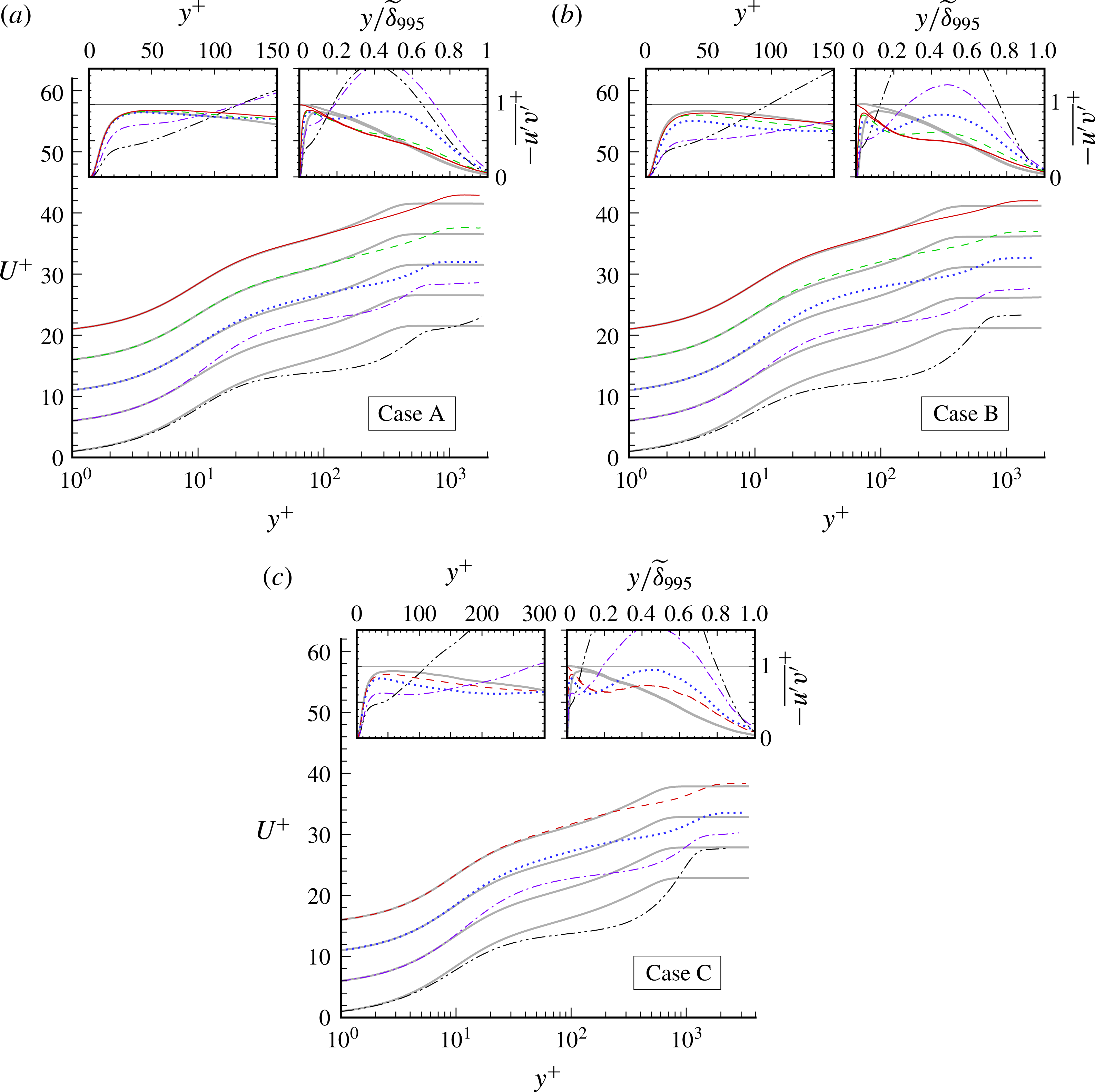
The effect of the APG on the mean velocity in inner/wall units is shown in figure 9. The velocity gradient $\unicode[STIX]{x2202}U/\unicode[STIX]{x2202}y$ outside the turbulent region is apparent. The present results do not support the proposal that the ZPG log law will survive when the maximum shear stress is less than 1.5 times the wall value (see stress profiles in inset plots), or when the magnitude of $p^{+}$ is less than 0.050 (denoted by $+$ symbols in figure 9 a–c); see for example Simpson (Reference Simpson1989) and Driver (Reference Driver1991). The deviation from the (nominally) logarithmic ZPG profile depends upon the Reynolds number and even more on the strength/duration of the APG. The controlling influence of the pressure gradient is revealed by its effect upon the $-\overline{u^{\prime }v^{\prime }}$ shear stress. The abrupt deceleration imposed for Case A has little impact upon the shape of the $-\overline{u^{\prime }v^{\prime }}$ profile (typical of ZPG conditions; see upper-left inset in figure 9 a), since the wall shear-stress reduction for this case has too little time to diffuse into the outer-layer turbulence (and the magnitude and duration of the outer-layer $\unicode[STIX]{x2202}\overline{v}/\unicode[STIX]{x2202}y$ strain are too small to effect significant $-\overline{u^{\prime }v^{\prime }}$ production; cf. Coleman, Kim & Spalart Reference Coleman, Kim and Spalart2003) before the mean skin friction changes sign, relative to the less-sudden APGs of Cases B and C; contrast the fuller $-\overline{u^{\prime }v^{\prime }}$ versus $y/\unicode[STIX]{x1D6FF}_{995}$ profiles in figure 9(b,c). These shear-stress changes are accompanied by departures from the log profile of the mean velocity that are quite general (rather than progressive; cf. Galbraith et al. Reference Galbraith, Sjolander and Head1977), roughly beginning at a given $y^{+}$ for each case, rather than a given $y/\unicode[STIX]{x1D6FF}$ , plausibly correlated with the different values of $p^{+}$ . A visual inspection of these profiles could lead to the interpretation that they still contain a logarithmic layer, but one with lower value of the von Kármán constant $\unicode[STIX]{x1D705}$ . We resist such interpretations, not having any evidence of these putative log layers lengthening with Reynolds number the way they do in ZPG. This is a reminder of the difficulty in defining equivalent flows at different Reynolds numbers when strong pressure gradients are at play. (Skote & Henningson (Reference Skote and Henningson2002) advocate an alternative perspective, and propose a log-law profile for both attached and separated cases.)

The common practice of mapping the magnitude of $U^{+}$ at $y^{+}=50$ versus $p^{+}$ to quantify PG-induced deviations from the log law (see for example Johnstone et al. 2010) is nowadays complicated by the emerging consensus that a purely logarithmic profile should not be expected, if at all, below $y^{+}$ of a few hundred – Marusic et al. (Reference Marusic, Monty, Hultmark and Smits2013) propose $y^{+}=3\sqrt{u_{\unicode[STIX]{x1D70F}}\unicode[STIX]{x1D6FF}/\unicode[STIX]{x1D708}}$ as the minimum, which is about 80 at the ZPG reference station for Case C – to say nothing about the current uncertainty in the value of $\unicode[STIX]{x1D705}$ , or the debate about its universality. We note that for Case C, opposite impressions are given by the behaviour of $U^{+}$ at $y^{+}=50$ and at $y^{+}=100$ , initially decreasing for the former and increasing for the latter. Despite these complications, we shall see below that the log law tends to be at least as insensitive to pressure gradients as other near-wall quantities such as the mixing length or eddy viscosity.

Figure 10.

(a,b) Mean-velocity profiles at (no symbols) separation and (symbols) reattachment, (a) with respect to $U_{\infty }$ and $Y$ , and (b) in Stratford scaling: - - - - (blue), Case A; — ⋅ — (green), Case B; —— (red), Case C; $\cdots \cdots$  (in b), Stratford’s (Reference Stratford1959) square-root-law $U^{-}=B\sqrt{y^{-}}+C$ , with $(B,C)=(2.5,-2.2)$ (Coleman et al. Reference Coleman, Pirozzoli, Quadrio and Spalart2017), where $U^{-}=U/u_{p}$ , $y^{-}=yu_{p}/\unicode[STIX]{x1D708}$ and $u_{p}^{3}=\unicode[STIX]{x1D708}\text{d}(\overline{p}_{wall}/\unicode[STIX]{x1D70C})/\text{d}x$ . Inset plot in (b) contains $-(\,\overline{u^{\prime }v^{\prime }}\,)^{-}=-\overline{u^{\prime }v^{\prime }}/u_{p}^{2}$ profiles: — ⋅ ⋅ — (dark), $-(\,\overline{u^{\prime }v^{\prime }}\,)^{-}=y^{-}$ idealisation. (c–f) Contours of (c) $B\sqrt{y^{-}}+C$ , and local $U^{-}$ for Cases (d) A, (e) B and (f) C. Dark solid vertical lines in (d–f) indicate mean separation and reattachment stations. The Case C results have been locally averaged in $x$ .

Figure 10 displays velocity profiles in the separated region, specifically at separation and reattachment, for comparison with the scaling postulated by Stratford (Reference Stratford1959) (cf. Skote & Henningson Reference Skote and Henningson2002). From figure 10(a) we find that the profiles at the two points with zero mean skin friction do not have a universal shape when plotted versus $y/Y$ . A figure versus $y/\unicode[STIX]{x1D6FF}$ would bring them closer, but still, some have an inflection point and others do not. In contrast, when drawn in ‘Stratford units’ $y^{-}$ and $U^{-}$ (see figure 10 legend), the six profiles essentially collapse up to $y^{-}\approx 16$ , and follow the square-root law beginning around $y^{-}\approx 2$ . (Refer to Coleman et al. (Reference Coleman, Pirozzoli, Quadrio and Spalart2017) for a discussion of why the $y^{-}$ values are not very large, compared with values in the hundreds for the logarithmic law.) This is in spite of the fact that the $-\overline{u^{\prime }v^{\prime }}$ profiles at $C_{f}=0$ are not particularly close to the linear idealisation associated with the Stratford conditions, although they are closer at reattachment (symbols) than at separation (see inset plot in figure 10 b).

Figure 11.

Mean-velocity profiles after reattachment, for $y\leqslant Y$ . (a) Case A: — ⋅ ⋅ — (dark), $x/Y=2(p^{+}=-0.029)$ ; — ⋅ — (purple), $x/Y=3(p^{+}=-0.006)$ ; $\cdots \cdots$  (blue),  $x/Y=5(p^{+}=0.000)$ ; - - - - (green), $x/Y=9(p^{+}=0.000)$ ; —— (red), $x/Y=11(p^{+}=0.000;R_{\unicode[STIX]{x1D703}}=2360)$ ; —— (grey/shaded), $x/Y=-5$ ( $p^{+}=0.000$ ; cf. figure 9 a). (b) Case B: — ⋅ ⋅ — (dark), $x/Y=3(p^{+}=-0.039)$ ; — ⋅ — (purple), $x/Y=5(p^{+}=-0.019)$ ; $\cdots \cdots$  (blue),  $x/Y=7(p^{+}=-0.004)$ ; - - - - (green), $x/Y=9(p^{+}=-0.001)$ ; —— (red), $x/Y=11(p^{+}=-0.001;R_{\unicode[STIX]{x1D703}}=2145)$ ; —— (grey/shaded), $x/Y=-8$ ( $p^{+}=0.001$ ; cf. figure 9 b). ( $c$ ) Case C: — ⋅ ⋅ — (dark), $x/Y=3(p^{+}=-0.031)$ ; — ⋅ — (purple), $x/Y=5(p^{+}=-0.013)$ ; $\cdots \cdots$  (blue),  $x/Y=7(p^{+}=-0.0025)$ ; - - - - (red), $x/Y=8.65(p^{+}=-0.001;R_{\unicode[STIX]{x1D703}}=4040)$ ; —— (grey/shaded), $x/Y=-9.5$ ( $p^{+}=0.000$ ; cf. figure 9 c). Profiles in (a–c) have been shifted five units in vertical scale above the one upstream, plotted below it. Inset plots in (a–c) contain $-\overline{u^{\prime }v^{\prime }}$ shear-stress profiles; total stress $\unicode[STIX]{x1D70F}/\unicode[STIX]{x1D70C}=-\overline{u^{\prime }v^{\prime }}+\unicode[STIX]{x1D708}\,\unicode[STIX]{x2202}\,\overline{u}/\unicode[STIX]{x2202}y$ also shown in right-hand-side subplots, for ZPG-reference and furthest-downstream stations (only).

Perhaps the most significant attribute of the collapse observed for the mean velocity is that it is so well approximated by the square-root law with slope and intercept coefficients taken from an independent DNS study in Couette–Poiseuille flow (using a channel-flow code; Coleman et al. Reference Coleman, Pirozzoli, Quadrio and Spalart2017). That flow has streamwise invariant statistics and sustained zero skin friction in the $x$ direction, in contrast with the present one, and was deemed to give Stratford scaling and square-root behaviour a possibly atypical chance of success (Stratford’s flow was different still, with sustained zero skin friction but rapid boundary-layer growth in $x$ ). The scaling appears to be very robust, the flow being dominated by the pressure gradient, which is the foundation of the Stratford units in the absence of a friction velocity. Figure 10(d–f) display contours of $U^{-}$ in $(x,\sqrt{y^{-}})$ axes, to compare with contours of the square-root law shown in figure 10(c). They show that between separation and reattachment – where due to the displacement effect, $\text{d}P/\text{d}x$ is approximately constant (see figure 3 b) – even though the negative skin friction is not strong, the quantity $U^{-}$ deviates appreciably from the square-root law, especially in Cases A and C. Thus, the law is valid strictly only at two locations. Here as in the Couette–Poiseuille flow, we view this as a notable success of turbulence theory.

The weakness of the backflow magnitude – for example, for Case C, at $x/Y=-0.5$ the minimum $\overline{u}$ is $-0.004U_{\infty }$ – is revealed by the fact that the near-wall mean-velocity profiles in local wall units deviate from the linear $U^{+}=y^{+}$ asymptote very close to the wall, below $y^{+}=0.5$ (cf. the corresponding profiles in figure 10 of Dianat & Castro Reference Dianat and Castro1989, for a more-deeply separated case). Nevertheless, the present reverse-flow profiles (not shown) are all reasonably well approximated by the expression proposed by Simpson (1983), $U/U_{N}=A[y/N-\ln (y/N)-1]-1$ (where $U_{N}$ is the magnitude of the maximum negative velocity and $N$ the distance from the wall at which it is found), provided $A\approx 0.9$ rather than Simpson’s original $A=0.3$ , or the $A=0.235$ found by Dianat & Castro (Reference Dianat and Castro1989) to best fit their results (see also Dianat & Castro Reference Dianat and Castro1991). The implications of this rather large variation for $A$ regarding the validity and universality of the $U_{N}$ scaling are at present not clear.

The recovery toward the ZPG state downstream of the bubble is documented in figure 11, in terms of the mean velocity in local wall units. The present results differ from those found by Castro & Epik (Reference Castro and Epik1998) downstream of their separation bubble, in that rather than a monotonic approach from below, here there is an overshoot in the log law for all three cases before the ZPG profile is recovered (cf. Mohammed-Taifour Reference Mohammed-Taifour2017). (The shaded curves in figure 11 a–c are from the ZPG reference station, upstream of the bubble; figure 5 a.) The source of this difference is likely to be that in the Castro & Epik experiment the recovering (or more accurately, developing) turbulent layer is initiated by a transitioning laminar separation bubble, in contrast to the APG/FPG-induced turbulent separation of a well-developed ZPG layer considered here. On the other hand, the DNS and the Castro & Epik experiment are similar in that the inner/logarithmic (but not the outer/wake) region of a ZPG is recovered about $10\unicode[STIX]{x1D6FF}_{r}$ downstream of reattachment, where $\unicode[STIX]{x1D6FF}_{r}$ is the layer thickness at reattachment. The solid lines in figure 11(a,b), and the dashed lines in figure 11(c) (i.e. the last stations unaffected by the outflow fringe for each case) correspond respectively to $(x-x_{r})/\unicode[STIX]{x1D6FF}_{r}=11.5$ (A), 9.8 (B) and 9.1 (C), where $x_{r}$ is the reattachment location (equal to $0.43Y$ for A, $0.21Y$ for B and $0.42Y$ for C), and $\unicode[STIX]{x1D6FF}_{r}$ is taken as $\widetilde{\unicode[STIX]{x1D6FF}}_{995}$ at $x=x_{r}$ (see figure 8 b). Another common feature of the experiment and the DNS is the very slow development of the outer region of the mean velocity: the outer-layer Clauser parameter $G=(2/C_{f})^{1/2}(H-1)/H$ at the furthest downstream ZPG stations ( $x/Y=12.5$ , 11 and 8.65, respectively, for Cases A, B and C) is $G=5.85$ , 5.2 and 5.0 – all well below the ZPG value of 6.8 found by Coles (Reference Coles1962). Castro & Epik observed $G=5.9$ at their farthest-downstream measuring station. They also found that $-\overline{u^{\prime }v^{\prime }}/u_{\unicode[STIX]{x1D70F}}^{2}$ recovers even more slowly than the outer-layer $U^{+}$ does, and that it tends to first settle to a level lower than the pure ZPG profile at comparable Reynolds number, before it rises very slowly toward the latter. Comparable behaviour is seen here, in that $-\overline{u^{\prime }v^{\prime }}/u_{\unicode[STIX]{x1D70F}}^{2}$ at a given $y/\unicode[STIX]{x1D6FF}_{995}$ is significantly less at the final prefringe locations than at the reference ZPG station from upstream (indicated in figure 11 by the solid grey/shaded curves); see for example the pronounced ‘divot’ relative to the ZPG profile in the Case B stress below $y/\unicode[STIX]{x1D6FF}_{995}\approx 0.5$ , in the right-hand-side subplot in figure 11(b). We conclude that in none of the three DNS cases does the layer reach the canonical, fully ZPG, state before it leaves the domain. The eventual development of a standard ZPG layer well upstream of the bubble, from the distorted/recovering turbulence, is another reminder of the success of the fringe treatment.

3.4 TKE budget

In addition to information about the downstream development of the individual terms in the TKE budget, which is offered as an aid to modellers attempting to replicate this flow, the following results underline the importance of exercising care when transferring concepts and intuition developed in thin shear layers to flows with streamline divergence/convergence, even when it is relatively mild.

Figure 12.

TKE budget for Case C: (a) TKE, $k=(1/2)\overline{u_{i}^{\prime }u_{i}^{\prime }}$ ; (b)  ${\mathcal{D}}k/{\mathcal{D}}t=\overline{u}\,\unicode[STIX]{x2202}k/\unicode[STIX]{x2202}x+\overline{v}\,\unicode[STIX]{x2202}k/\unicode[STIX]{x2202}y$ ; (c) production rate, ${\mathcal{P}}_{k}=-\overline{u_{i}^{\prime }u_{j}^{\prime }}\unicode[STIX]{x2202}\overline{u}_{i}/\unicode[STIX]{x2202}x_{j}$ ; (d) (minus) dissipation rate, $-\unicode[STIX]{x1D716}_{k}=-\unicode[STIX]{x1D708}\overline{(\unicode[STIX]{x2202}u_{i}^{\prime }/\unicode[STIX]{x2202}x_{j})(\unicode[STIX]{x2202}u_{i}^{\prime }\unicode[STIX]{x2202}x_{j})}$ ; (e) turbulent transport, ${\mathcal{T}}_{k}=-(1/2)\unicode[STIX]{x2202}\overline{u_{i}^{\prime }u_{i}^{\prime }u_{j}^{\prime }}/\unicode[STIX]{x2202}x_{j}$ ; (f) velocity–pressure-gradient correlation, $\unicode[STIX]{x1D6F1}_{k}=-\overline{(u_{i}^{\prime }/\unicode[STIX]{x1D70C})\unicode[STIX]{x2202}p^{\prime }/\unicode[STIX]{x2202}x_{i}}$ . (In ZPG regions, extrema for ${\mathcal{P}}_{k}$ , $-\unicode[STIX]{x1D716}_{k}$ and $\unicode[STIX]{x1D6F1}_{k}$ , which lie outside the limits shown here, are located very near the wall; cf. figure 6, and note that at $x/Y=-9.5$ , $y^{+}=50$ corresponds to $y/Y=0.014$ .) Black curves are mean streamlines; solid white vertical lines indicate mean separation and reattachment stations. White symbols denote 99.5 %-boundary-layer thickness $\widetilde{\unicode[STIX]{x1D6FF}}_{995}$ . Broken white curve in (a) is mean dividing streamline of separation bubble. Broken lines in (c) trace contours of ${\mathcal{P}}_{k}/\unicode[STIX]{x1D716}_{k}=1$ , 1.5 and 2, while grey/shaded regions in (c) correspond to ${\mathcal{P}}_{k}<0$ (minimum value is $-7\times 10^{-5}$ ). All terms computed directly, except $\unicode[STIX]{x1D6F1}_{k}$ , which is inferred from budget imbalance. TKE and budget terms respectively normalised by $U_{\infty }^{2}$ and $U_{\infty }^{3}/Y$ . Results have been locally averaged in  $x$ .

For all three cases, a local TKE maximum (in addition to the near-wall peak in the ZPG layer) occurs in the region above the upstream portion of the mean separation bubble. For Case C, the peak (which is nearly the same magnitude, in units of $U_{\infty }^{2}$ , as the near-wall ZPG-reference value; cf. figure 6 a) is directly above the mean separation location, $x/Y=-1.43$ (figure 12 a). This is in contrast to turbulent separation induced by surface curvature, such as in the rounded-step flow studied by Bentaleb, Lardeau & Leschziner (Reference Bentaleb, Lardeau and Leschziner2012), where the TKE peak is larger (with respect to $U_{\infty }^{2}$ ) and further downstream. The TKE growth or decay along mean streamlines – and thus this local maximum – is largely controlled by the imbalance between the production ${\mathcal{P}}_{k}$ , dissipation $\unicode[STIX]{x1D716}_{k}$ and turbulent transport ${\mathcal{T}}_{k}$ terms. The velocity–pressure-gradient correlation $\unicode[STIX]{x1D6F1}_{k}$ is quite small except adjacent to the wall, where it acts as a source (cf. figure 6 b). (Recall however that the pressure term acts as a strong sink for the Reynolds shear stress $-\overline{u^{\prime }v^{\prime }}$ across the layer (Spalart Reference Spalart1988).) Our focus here will be upon outer-layer regions.

The turbulent transport ${\mathcal{T}}_{k}$ (figure 12 e) tends to spread TKE down the TKE gradients, both toward and away from the wall. It makes a particularly important contribution toward the outer edge of the turbulent layer, accounting for nearly all of the positive ${\mathcal{D}}k/{\mathcal{D}}t$ in the APG and especially FPG regions.

The evolution of the production term correlates with that of the $x$ -component normal Reynolds stress $\overline{u^{\prime }u^{\prime }}$ . For example, in the $\unicode[STIX]{x2202}\overline{u}/\unicode[STIX]{x2202}x=\unicode[STIX]{x1D61A}_{11}<0$ (APG) region, ${\mathcal{P}}_{k}$ ( $=-(\overline{u^{\prime }u^{\prime }}-\overline{v^{\prime }v^{\prime }})\,\unicode[STIX]{x1D61A}_{11}-2\overline{u^{\prime }v^{\prime }}\,\unicode[STIX]{x1D61A}_{12}$ ) grows as $\overline{u^{\prime }u^{\prime }}$ does, and conversely in the FPG region. The $\overline{u^{\prime }u^{\prime }}$ component also contributes to a reduction in the $-\overline{u^{\prime }v^{\prime }}$ stress, through the latter’s production, $-\unicode[STIX]{x1D617}_{12}=\overline{u^{\prime }u^{\prime }}\,\unicode[STIX]{x2202}\overline{v}/\unicode[STIX]{x2202}x+\overline{v^{\prime }v^{\prime }}\,\unicode[STIX]{x2202}\overline{u}/\unicode[STIX]{x2202}y$ , coupled with the present transpiration profile, with its negative $\text{d}V_{top}/\text{d}x$ (figure 3 a). For Case A, with its sudden APG/FPG, $|\unicode[STIX]{x2202}\overline{v}/\unicode[STIX]{x2202}x|$ is large enough to produce negative $-\overline{u^{\prime }v^{\prime }}$ in the outer layer, which significantly reduces the TKE production there, via the $-2\overline{u^{\prime }v^{\prime }}\,\unicode[STIX]{x1D61A}_{12}$ term. In SC97, Skote & Henningson (Reference Skote and Henningson2002) and Abe et al. (Reference Abe, Mizobuchi, Matsuo and Spalart2012) (but not for Case A), this suppression was strong enough to yield a pocket of negative ${\mathcal{P}}_{k}$ in the outer layer, above the separation bubble. (The negative ${\mathcal{P}}_{k}$ in the free-stream, above $y=\widetilde{\unicode[STIX]{x1D6FF}}_{995}$ , seen in figure 12 c is statistically insignificant.) For Cases B and C, with their more gradual pressure gradients, $-\overline{u^{\prime }v^{\prime }}$ is everywhere positive, and the $-\overline{u^{\prime }v^{\prime }}<0$ excursion of ${\mathcal{P}}_{k}$ does not occur (cf. figure 12 c).

Figure 13.

Case C contours of mean (a) strain rate $\sqrt{2\unicode[STIX]{x1D61A}_{ij}\unicode[STIX]{x1D61A}_{ij}}$ , (b) stream(line)wise strain rate $\sqrt{4\unicode[STIX]{x1D61A}_{11}^{\ast }\unicode[STIX]{x1D61A}_{11}^{\ast }}$ , (c) cross-stream Reynolds shear stress $-\overline{u_{\ast }^{\prime }v_{\ast }^{\prime }}$ , (d) cross-stream strain rate $\sqrt{4\unicode[STIX]{x1D61A}_{12}^{\ast }\unicode[STIX]{x1D61A}_{12}^{\ast }}$ , (e) Reynolds shear stress $-\overline{u^{\prime }v^{\prime }}$ , (f) productive shear stress $-\overline{u^{\prime }v^{\prime }}_{prod}={\mathcal{P}}_{k}/\sqrt{2\unicode[STIX]{x1D61A}_{ij}\unicode[STIX]{x1D61A}_{ij}}$ , (g) turbulence stress–energy ratio $-\overline{u^{\prime }v^{\prime }}/k$ and (h) turbulence-to-mean energy transfer efficiency $a_{1,prod}=({\mathcal{P}}_{k}/\sqrt{2\unicode[STIX]{x1D61A}_{ij}\unicode[STIX]{x1D61A}_{ij}})/k$ . Quantities with ‘ $\ast$ ’ super- or subscripts are defined with respect to local Cartesian coordinates $(x_{1}^{\ast },x_{2}^{\ast })$ , aligned with ( $x_{1}^{\ast }$ ) and normal to ( $x_{2}^{\ast }$ ) mean streamlines (solid black curves). Solid white vertical lines mark mean separation and reattachment stations. White symbols denote 99.5 %-boundary-layer thickness $\widetilde{\unicode[STIX]{x1D6FF}}_{995}$ . Grey regions indicate values outside the colour bar range shown for each figure.

From the above, we see that the mean $x$ -wise compression/expansion $\unicode[STIX]{x1D61A}_{11}$ provides a direct/explicit contribution to ${\mathcal{D}}k/{\mathcal{D}}t$ , through the presence of this strain component in ${\mathcal{P}}_{k}$ . However, we are not considering a thin shear flow exactly aligned with the $x$ axis. This explicit dependence of the TKE production on the mean strain is more naturally viewed in terms of the compression/expansion $\unicode[STIX]{x1D61A}_{11}^{\ast }=-\unicode[STIX]{x1D61A}_{22}^{\ast }$ relative to Cartesian axes $(x_{1}^{\ast },x_{2}^{\ast })=(x_{\ast },y_{\ast })$ aligned with the local mean-velocity vector $(\overline{u}_{1},\overline{u}_{2})=(\overline{u},\overline{v})$ , with ${\mathcal{P}}_{k}$ rewritten as $=-(\overline{u_{\ast }^{\prime }u_{\ast }^{\prime }}-\overline{v_{\ast }^{\prime }v_{\ast }^{\prime }})\,\unicode[STIX]{x1D61A}_{11}^{\ast }-2\overline{u_{\ast }^{\prime }v_{\ast }^{\prime }}\,\unicode[STIX]{x1D61A}_{12}^{\ast }$ . (In these ‘starred’, local stream(line)-wise coordinates, we have for example, that the streamwise rate of strain is $\unicode[STIX]{x1D61A}_{11}^{\ast }=(\overline{u}\,\overline{u}\unicode[STIX]{x1D61A}_{11}+2\overline{u}\,\overline{v}\unicode[STIX]{x1D61A}_{12}+\overline{v}\,\overline{v}\unicode[STIX]{x1D61A}_{22})/(\overline{u}\,\overline{u}+\overline{v}\,\overline{v})$ (recall $\unicode[STIX]{x1D61A}_{ij}^{\ast }=\unicode[STIX]{x1D613}_{ip}\unicode[STIX]{x1D613}_{jq}\unicode[STIX]{x1D61A}_{pq}$ , where $\unicode[STIX]{x1D613}_{ij}$ is the cosine of the angle between the $x_{i}^{\ast }$ and $x_{j}$ axes), and the cross-stream $x_{1}^{\ast }$ – $x_{2}^{\ast }$ Reynolds shear stress is $-\overline{u_{\ast }^{\prime }v_{\ast }^{\prime }}=-((\overline{u}\,\overline{u}-\overline{v}\,\overline{v})\overline{u^{\prime }v^{\prime }}-\overline{u}\,\overline{v}(\overline{u^{\prime }u^{\prime }}-\overline{v^{\prime }v^{\prime }}))/(\overline{u}\,\overline{u}+\overline{v}\,\overline{v})$ .) The shear stresses referred to the two sets of axes are appreciably different even though the streamline inclination is only of the order of 0.125 radians: compare figures 13(c) and 13(e).

In view of the large changes effected by $\text{d}P/\text{d}x$ , it is somewhat surprising that the magnitude of the ‘extra’ strain $\unicode[STIX]{x1D61A}_{11}^{\ast }$ (‘extra’ in the sense of being in addition to the primary/cross-stream shear component $\unicode[STIX]{x1D61A}_{12}^{\ast }$ ; Bradshaw Reference Bradshaw1988) that it induces is such a small fraction of the total (compare figures 13 b with 13 a and 13 d). The major influence of $\unicode[STIX]{x1D61A}_{11}^{\ast }$ is more indirect, as we shall now see. (The magnitude of the streamline curvature, $\unicode[STIX]{x2202}\overline{v}_{\ast }/\unicode[STIX]{x2202}x_{\ast }$ ( $=(\overline{\unicode[STIX]{x1D714}}_{z}+2\unicode[STIX]{x1D61A}_{12}^{\ast })/2$ ), which is another of Bradshaw’s extra strains, is even smaller than $|\unicode[STIX]{x1D61A}_{11}^{\ast }|$ – to the point $\unicode[STIX]{x2202}\overline{v}_{\ast }/\unicode[STIX]{x2202}x_{\ast }$ would not register when plotted using the contour levels employed in figure 13 b. Evidently, although the streamline inclination is not negligible – recall the large differences between $-\overline{u^{\prime }v^{\prime }}$ and $-\overline{u_{\ast }^{\prime }v_{\ast }^{\prime }}$ observed above – its variation with $x$ is rather weak.)

An example of an indirect effect of $\unicode[STIX]{x1D61A}_{11}^{\ast }$ is provided by the behaviour of the $-2\overline{u_{\ast }^{\prime }v_{\ast }^{\prime }}\unicode[STIX]{x1D61A}_{12}^{\ast }$ contribution to ${\mathcal{P}}_{k}$ . From figure 13(c,d) we find a tendency for the streamwise increases associated with the two local maxima of the cross-stream stress $-\overline{u_{\ast }^{\prime }v_{\ast }^{\prime }}$ to offset the general streamwise decrease of $\unicode[STIX]{x1D61A}_{12}^{\ast }$ , such that their combination to ${\mathcal{P}}_{k}$ produces a net decrease that is weaker than the streamwise evolution of $\unicode[STIX]{x1D61A}_{12}^{\ast }$ alone would imply. Concerning the latter, since the magnitude of $\unicode[STIX]{x1D61A}_{12}^{\ast }$ is quite close to that of the streamwise vorticity $\overline{\unicode[STIX]{x1D714}}_{z}$ (not shown), which points to the dominance of the cross-stream gradient of the mean streamwise velocity $\unicode[STIX]{x2202}\overline{u}_{\ast }/\unicode[STIX]{x2202}y_{\ast }$ , the decrease in $\unicode[STIX]{x1D61A}_{12}^{\ast }$ can be associated with the viscous and especially turbulent diffusion terms in the $\overline{\unicode[STIX]{x1D714}}_{z}$ transport equation. These diffusion terms can be interpreted as further indirect effects of the $\unicode[STIX]{x1D61A}_{11}^{\ast }=-\unicode[STIX]{x1D61A}_{22}^{\ast }$ straining. As initially noted by Bradshaw (Reference Bradshaw1988), these types of indirect extra-strain effects are of greater importance than one might deduce from information such as that shown in figure 13(b).

Regarding the rate-of-dissipation $\unicode[STIX]{x1D716}_{k}$ , the third of the major terms in the outer-layer balance, we note the tendency for it to mitigate the production, with ${\mathcal{P}}_{k}/\unicode[STIX]{x1D716}_{k}$ of order one throughout the bulk of the layer (see broken-line contours in figure 12 c). On the other hand, the dissipation is observed to follow the mean streamlines (i.e. satisfy ${\mathcal{D}}\unicode[STIX]{x1D716}_{k}/{\mathcal{D}}t\approx 0$ ) better than production does, especially downstream of reattachment (compare the ${\mathcal{P}}_{k}/\unicode[STIX]{x1D716}_{k}$ and ${\mathcal{P}}_{k}$ contours in figure 12 c). This is not unexpected, $\unicode[STIX]{x1D716}_{k}$ being dominated by the small scales of the turbulence and not directly impacted by the pressure field. Accounting for this ‘drift’ of ${\mathcal{P}}_{k}$ across the streamlines into the FPG outer layer, which is consistent with the rise of ${\mathcal{P}}_{k}/\unicode[STIX]{x1D716}_{k}$ for $x>0$ , the present behaviour aligns with the standard/Kolmogorov view of the energy cascade, in that ${\mathcal{P}}_{k}<\unicode[STIX]{x1D716}_{k}$ begins to fall along mean streamlines within the APG, just downstream of the peak-TKE location – indicating the rate of dissipation is not immediately affected by the reduced TKE at larger scales (cf. Abe et al. Reference Abe, Mizobuchi, Matsuo and Spalart2012).

Although it is convenient to consider the Reynolds stresses and TKE budget with regard to the $x$ – $y$ , wall-parallel/wall-normal, coordinate system, this can produce a partial and thus misleading picture, especially in regions far from the wall, where streamline slope is not negligible, and even the streamline direction does not necessarily give a rigorous ‘most relevant’ set of axes. We have already observed the example provided by the significant differences between the Reynolds shear stress in streamline axes, $-\overline{u_{\ast }^{\prime }v_{\ast }^{\prime }}$ (figure 13 c) and in $x$ – $y$ axes, $-\overline{u^{\prime }v^{\prime }}$ (figure 13 e). A further example is provided by what could be called the ‘effective’ or ‘productive’ stress $-\overline{u^{\prime }v^{\prime }}_{prod}$ , formulated in terms of the mean-to-turbulence energy transfer ${\mathcal{P}}_{k}$ , which is independent of axes. Since the rate of TKE production represents the work done against the mean-rate-of-strain field by the turbulent stresses, we define $-\overline{u^{\prime }v^{\prime }}_{prod}$ as the characteristic turbulent-shear-stress field given by the scalar ratio ${\mathcal{P}}_{k}/\sqrt{2\unicode[STIX]{x1D61A}_{ij}\unicode[STIX]{x1D61A}_{ij}}$ (which in a parallel flow, with $\overline{u}=\overline{u}(y)$ , reduces to $-\overline{u^{\prime }v^{\prime }}$ ). Figure 13(e,f) implies that $-\overline{u^{\prime }v^{\prime }}$ and $-\overline{u^{\prime }v^{\prime }}_{prod}$ are very different, to the point that their outer-layer maxima are on the opposite sides of the bubble. (The $-\overline{u^{\prime }v^{\prime }}_{prod}$ and $-\overline{u_{\ast }^{\prime }v_{\ast }^{\prime }}$ fields are qualitatively similar, although not identical, especially downstream of reattachment; figure 13 f,c.) Moreover, the streamline slope does not have to be extreme for the differences to be meaningful. This can be seen when examining the so-called Reynolds-stress structure parameter, $a_{1}=-\overline{u^{\prime }v^{\prime }}/k$ (Bradshaw, Ferris & Atwell Reference Bradshaw, Ferris and Atwell1967). This stress/TKE ratio can be interpreted as a measure of the ‘efficiency’ with which the turbulence alters (transfers) the mean momentum (and energy) in a parallel flow. Figure 13(g) reveals the frequently observed reduction of $a_{1}$ in the APG region (Spalart & Watmuff Reference Spalart and Watmuff1993), which is typically assumed to imply a reduction in the efficiency of the turbulence/mean transfer process (e.g. Coleman et al. Reference Coleman, Kim and Spalart2003). (The stress/energy ratio based on the Reynolds stress in streamline coordinates, $a_{1}^{\ast }=-\overline{u_{\ast }^{\prime }v_{\ast }^{\prime }}/k$ , also reveals a downstream reduction, albeit one slower than for $a_{1}$ .) In fact, the productive stress/energy ratio $a_{1,prod}=-\overline{u^{\prime }v^{\prime }}_{prod}/k$ (figure 13 h) demonstrates the opposite, that the effect of the APG is an increase of relative mean-to-turbulence energy transfer – and that this increase is observed in regions where the streamline slope is quite small. Also noteworthy is the ‘quiet zone of inefficiency’ above the bubble, where $a_{1,prod}\approx 0.2$ .

3.5 Pressure-gradient dependence of near-wall length scales

We now turn attention to the behaviour of various length scales associated with near-wall turbulence, and in particular how they are affected by pressure gradient. This exercise extends our work on turbulent Couette–Poiseuille (C–P) flow DNS, for which one side is effectively an APG layer, the other effectively an FPG (Johnstone, Coleman & Spalart Reference Johnstone, Coleman and Spalart2010; Coleman, Garbaruk & Spalart Reference Coleman, Garbaruk and Spalart2015). There we found the length scale defined by the logarithmic law tends to be less sensitive to wall-normal shear-stress gradients than other alternatives. This line of thinking was initiated by Galbraith & Head (Reference Galbraith and Head1975) and Galbraith et al. (Reference Galbraith, Sjolander and Head1977). The question before us now is the extent to which this parallel-flow observation also holds for the spatially developing case. The implications for turbulence modelling and theory are significant.

For context, recall that one finds in the literature at least three conjectured relationships between the wall-normal derivative of the mean velocity $\text{d}U/\text{d}y$ and the primary shear stress $-\overline{u^{\prime }v^{\prime }}$ , the two quantities at the core of turbulence modelling in unidirectional flows. Based on the assumption of a constant-stress (‘pure Couette’) region, and presented in terms of length scales, to allow direct comparisons, these relationships include the one leading to the logarithmic law of the wall for the velocity, namely

(3.5) $$\begin{eqnarray}\ell _{U}=\frac{u_{\unicode[STIX]{x1D70F}}}{\text{d}U/\text{d}y}=\unicode[STIX]{x1D705}y,\end{eqnarray}$$

where $\unicode[STIX]{x1D705}$ is again the von Kármán constant and $u_{\unicode[STIX]{x1D70F}}=\sqrt{\unicode[STIX]{x1D70F}_{w}/\unicode[STIX]{x1D70C}}$ the wall friction velocity. In terms of eddy viscosity $\unicode[STIX]{x1D708}_{t}\equiv -\overline{u^{\prime }v^{\prime }}/(\text{d}U/\text{d}y)$ , we also have

(3.6) $$\begin{eqnarray}\ell _{\unicode[STIX]{x1D708}_{t}}=\frac{\unicode[STIX]{x1D708}_{t}}{u_{\unicode[STIX]{x1D70F}}}=\frac{-\overline{u^{\prime }v^{\prime }}/u_{\unicode[STIX]{x1D70F}}}{\text{d}U/\text{d}y}=\unicode[STIX]{x1D705}y,\end{eqnarray}$$

while consideration of the mixing length $\ell _{t}\equiv (\unicode[STIX]{x1D708}_{t}/(\text{d}U/\text{d}y))^{1/2}$ gives

(3.7) $$\begin{eqnarray}\ell _{t}=\frac{\sqrt{-\overline{u^{\prime }v^{\prime }}}}{\text{d}U/\text{d}y}=\unicode[STIX]{x1D705}y.\end{eqnarray}$$

Yet another scale can be based on the rate of TKE production (Coleman et al. Reference Coleman, Garbaruk and Spalart2015),

(3.8) $$\begin{eqnarray}\ell _{{\mathcal{P}}}=\frac{u_{\unicode[STIX]{x1D70F}}^{3}}{-\overline{u^{\prime }v^{\prime }}\text{d}U/\text{d}y}=\unicode[STIX]{x1D705}y.\end{eqnarray}$$

The four formulae differ by various powers of the ratio $-\overline{u^{\prime }v^{\prime }}/u_{\unicode[STIX]{x1D70F}}^{2}$ . Since $-\overline{u^{\prime }v^{\prime }}=u_{\unicode[STIX]{x1D70F}}^{2}$ in a constant-stress layer outside the viscous region, all four expressions are equivalent under pure Couette conditions (see figure 4 in Johnstone et al. Reference Johnstone, Coleman and Spalart2010). None of the four has a systematic derivation. (See Skote & Wallin (Reference Skote and Wallin2016) for a review of current wall-damping functions, and an attempt to generalise them into a single model applicable to decelerating and separated flows.) With pressure gradient, $-\overline{u^{\prime }v^{\prime }}$ deviates from $u_{\unicode[STIX]{x1D70F}}^{2}$ , even outside the viscous buffer layer, and the proposals conflict, so that at best one of the four will remain effective. The four will produce a ‘fan’ of results in the order (3.8)–(3.5)–(3.7)–(3.6): that is, $\ell _{{\mathcal{P}}}<\ell _{U}<\ell _{t}<\ell _{\unicode[STIX]{x1D708}_{t}}$ for APG, and $\ell _{{\mathcal{P}}}>\ell _{U}>\ell _{t}>\ell _{\unicode[STIX]{x1D708}_{t}}$ for FPG (or, in terms of $\ell _{U}$ , $(-\overline{u^{\prime }v^{\prime }}/u_{\unicode[STIX]{x1D70F}}^{2})^{-1}\ell _{U}\gtrless \ell _{U}\gtrless (-\overline{u^{\prime }v^{\prime }}/u_{\unicode[STIX]{x1D70F}}^{2})^{1/2}\ell _{U}\gtrless (-\overline{u^{\prime }v^{\prime }}/u_{\unicode[STIX]{x1D70F}}^{2})\ell _{U}$ .) This behaviour is confirmed in figure 14, which presents (3.5)–(3.8) for Case C at representative stations (with $\text{d}U/\text{d}y$ replaced by local $\unicode[STIX]{x2202}\overline{u}/\unicode[STIX]{x2202}y$ ), in that $\ell _{\unicode[STIX]{x1D708}_{t}}$ and $\ell _{{\mathcal{P}}}$ are the largest, respectively, in the APG and FPG regions. (For reference, the solid symbol in figure 14 denotes the local $0.15\widetilde{\unicode[STIX]{x1D6FF}}_{995}$ location, the height below which one might expect classical inertial sublayer relations to hold; cf. Marusic et al. Reference Marusic, Monty, Hultmark and Smits2013.) As required, the ordering is indeed tied to the magnitude of the $-\overline{u^{\prime }v^{\prime }}/u_{\unicode[STIX]{x1D70F}}^{2}$ ratio (see shear-stress inset plots in figures 9 and 11).

Figure 14.

Length scale variation for Case C at (a) $x/Y=-9.5$ , (b) $x/Y=-7$ , (c) $x/Y=-5$ , (d) $x/Y=5$ , (e) $x/Y=7$ and (f) $x/Y=8.65$ : ——, $\unicode[STIX]{x1D705}y$ , for $\unicode[STIX]{x1D705}=0.38$ and $0.41$ ; ▪, $y^{+}=0.15\,u_{\unicode[STIX]{x1D70F}}\,\widetilde{\unicode[STIX]{x1D6FF}}_{995}/\unicode[STIX]{x1D708}$ ; — ⋅ — (red), $\ell _{U}$ ; — ⋅ ⋅ — (green), $\ell _{\unicode[STIX]{x1D708}_{t}}$ ; - - - - (blue), $\ell _{t}$ ; $\cdots \cdots$  (violet),  $\ell _{{\mathcal{P}}}$ . Vertical lines in (wall-pressure) inset plots indicate streamwise station to which data in main plot correspond.

Because $-\overline{u^{\prime }v^{\prime }}/u_{\unicode[STIX]{x1D70F}}^{2}\leqslant 1$ at the ZPG station, unlike for pure Couette flow, there is a discernible difference between the length scales here. Figure 14(a) reveals a mild form of the expected FPG ordering ( $\ell _{{\mathcal{P}}}$ maximum, $\ell _{\unicode[STIX]{x1D708}_{t}}$ minimum) for the Case C ZPG reference state. An even larger difference with respect to the parallel C–P geometry – for which, on both the APG and FPG sides, $\ell _{U}$ is least sensitive to $\text{d}P/\text{d}x$ and agrees most closely with the $\unicode[STIX]{x1D705}y$ idealisation (Johnstone et al. Reference Johnstone, Coleman and Spalart2010; Coleman et al. Reference Coleman, Garbaruk and Spalart2015) – is that for the present flow the ‘winner’ regarding PG independence is not as clear (and is not $\ell _{{\mathcal{P}}}$ , despite the hints found in Spalart (Reference Spalart1988), as described in Coleman et al. (Reference Coleman, Garbaruk and Spalart2015)). The prevailing uncertainty over the value of $\unicode[STIX]{x1D705}$ has essentially no impact on the comparisons. (Neither does the use of the coordinate-dependent/parallel-flow definitions in (3.5)–(3.8): utilising the TKE-production-based quantities mentioned above instead – representing $\ell _{U}$ by $-u_{\unicode[STIX]{x1D70F}}/\overline{\unicode[STIX]{x1D714}}_{z}$ or $u_{\unicode[STIX]{x1D70F}}/(2\unicode[STIX]{x1D61A}_{ij}\unicode[STIX]{x1D61A}_{ij})^{1/2}$ , $\ell _{\unicode[STIX]{x1D708}_{t}}$ by ${\mathcal{P}}_{k}/(2\unicode[STIX]{x1D61A}_{ij}\unicode[STIX]{x1D61A}_{ij}u_{\unicode[STIX]{x1D70F}})$ , $\ell _{t}$ by ${\mathcal{P}}_{k}^{1/2}/(2\unicode[STIX]{x1D61A}_{ij}\unicode[STIX]{x1D61A}_{ij})^{3/2}$ and $\ell _{{\mathcal{P}}}$ by $u_{\unicode[STIX]{x1D70F}}^{3}/{\mathcal{P}}_{k}$ – has no effect on the ordering observed in figure 14, and in fact slightly amplifies the pressure-gradient dependence of all but $\ell _{U}$ .) Nevertheless, since at most of the stations the length scale fan tends to overlap most of the $\unicode[STIX]{x1D705}y$ target below the $0.15\widetilde{\unicode[STIX]{x1D6FF}}_{995}$ limit, and since $\ell _{U}$ and $\ell _{t}$ always lie within the ‘core’ of the fan, a case can be made that the log-law and mixing-length scales are more resilient to pressure gradients than the other two options. We also note the importance of the (upstream) flow history in the hysteresis between the APG and FPG regions, in the tendency for the lengths to depart from $\unicode[STIX]{x1D705}y$ at higher $y^{+}$ (and especially $y/\unicode[STIX]{x1D6FF}_{995}$ ) under an adverse gradient than under a FPG of comparable (in fact slightly weaker) magnitude, measured in local wall units (compare figures 14 c and 14 d). At $x/Y=5$ , long after reattachment, the deviations are still strong, well below $y=0.15\widetilde{\unicode[STIX]{x1D6FF}}_{995}$ . At the final station, quasi-ZPG conditions are again apparent, with slightly more pronounced FPG ordering, due to the sub-ZPG levels of $-\overline{u^{\prime }v^{\prime }}/u_{\unicode[STIX]{x1D70F}}^{2}$ mentioned in § 3.3. To appreciate the significance of these findings for RANS modelling, we note that algebraic models explicitly containing $\ell _{\unicode[STIX]{x1D708}_{t}}$ or $\ell _{t}$ such as Cebeci–Smith or Baldwin–Lomax are no longer in general use, but that wall functions based on $\ell _{U}$ are in use, and also that some transport-equation models (including Spalart–Allmaras) contain terms related to $\ell _{t}$ .

4.1 RANS grid and numerical details

Results were computed with the code CFL3D (Krist, Biedron & Rumsey Reference Krist, Biedron and Rumsey1998), developed at NASA. CFL3D is a multi-zone compressible RANS code that employs grid sequencing and multigrid to accelerate convergence to steady state. It is a finite-volume method, and uses third-order upwind-biased spatial differencing on the convective and pressure terms and second-order differencing on the viscous terms; it is globally second-order spatially accurate. The flux difference-splitting (FDS) method of Roe (Reference Roe1981) is employed to obtain fluxes at the cell faces. CFL3D is advanced in time via backward Euler, with an implicit three-factor approximate factorisation method. The turbulence equations are solved by default with a first-order advection scheme, although second-order is also available.

There are many RANS turbulence models available in CFL3D. For this work, we used Baldwin–Lomax (BL) (Baldwin & Lomax Reference Baldwin and Lomax1978), Spalart–Allmaras (SA) (Spalart & Allmaras Reference Spalart and Allmaras1994), Spalart–Allmaras with rotation-curvature correction (SARC) (Shur et al. Reference Shur, Strelets, Travin and Spalart2000), the ‘AB’ $k$ – $\unicode[STIX]{x1D716}$ model of Abid ( $k$ – $\unicode[STIX]{x1D716}$ ) (Abid Reference Abid1993), Menter’s shear-stress transport $k$ – $\unicode[STIX]{x1D714}$ (SST) (Menter Reference Menter1994) and the SSG/LRR-RSM-w2012 (Speziale–Sarkar–Gatski/Launder–Reece–Rodi differential Reynolds-stress model) Reynolds-stress transport (RST) (Eisfeld, Rumsey & Togiti Reference Eisfeld, Rumsey and Togiti2016). Because of the relatively low Reynolds number of this flow, we also used modified forms of SA and SARC, termed low- $Re$ SA and low- $Re$ SARC, respectively. These are the same as the original models, with the exception that the coefficient $C_{w2}$ has been increased from 0.3 to 1.0. This change yields somewhat higher skin friction for the ZPG flow leading up to separation. The original models were calibrated for higher $Re$ , and they tend to underpredict flat-plate skin friction when $Re$ is very low. Increasing $C_{w2}$ in SA increases the slope of $f_{w}$ with respect to $r\equiv \unicode[STIX]{x1D708}_{t}/(\unicode[STIX]{x1D705}^{2}y^{2}\unicode[STIX]{x2202}\overline{u}/\unicode[STIX]{x2202}y)$ at $r=1$ (i.e. in the log region, where $\unicode[STIX]{x1D708}_{t}=\unicode[STIX]{x1D705}u_{\unicode[STIX]{x1D70F}}y$ and $\unicode[STIX]{x2202}\overline{u}/\unicode[STIX]{x2202}y=u_{\unicode[STIX]{x1D70F}}/\unicode[STIX]{x1D705}y$ ), such that the SA destruction term is diminished in the outer layer, where $r<1$ (see figure 3 of Spalart & Allmaras Reference Spalart and Allmaras1994). Consequently, the total mixing across the layer, via enhanced $\unicode[STIX]{x1D708}_{t}$ , increases, leading to higher skin friction.

The turbulence models are not described in detail here; the reader is referred to the original references for their equations. In terms of a general overview, BL is an algebraic model that sees very little usage today (except by the hypersonics community). It is included here because it provides an example of poor results with far too early separation (the model, however, has the opposite trend for shock-induced separation). Similarly, $k$ – $\unicode[STIX]{x1D716}$ is not widely used for aerodynamic flows because of its poor characteristics, particularly for flows with APG. Here, it is included because it provides an opposite example of poor results with no separation. The other models, SA, SARC, SST and RST, are all considered state-of-the-art RANS models by today’s aerodynamics community. SA and SARC are one-equation transport models, SST is a two-equation transport model, and RST is a seven-equation transport model.

The fine grid size was $721\times 513$ . Medium grid size was $361\times 257$ (every other point of the fine grid in each coordinate direction). The grid extended from $x/Y=-12.15$ (upstream) to $x/Y=10.65$ (downstream). The top-wall boundary was located at $y/Y=1$ . Minimum normal spacing at the bottom wall was $\unicode[STIX]{x0394}y/Y=8\times 10^{-5}$ (fine grid) and $\unicode[STIX]{x0394}y/Y=16\times 10^{-5}$ (medium grid), corresponding to an average $\unicode[STIX]{x0394}y^{+}$ over the entire plate of approximately $\unicode[STIX]{x0394}y^{+}=0.2$ and $0.4$ , respectively. Solutions computed on both grids yielded only very minor differences in results. For example, the maximum change in separation or reattachment location for any model was less than $0.2Y$ , with maximum change in bubble length of approximately $0.3Y$ , or less than 2 %. Therefore, medium grids were used for the solutions shown here.

The reference (ZPG free-stream) Mach number was $M=0.1$ , and Reynolds number based on the reference velocity and height $Y$ ) was $Re=80\,000$ , to agree with Case C. The top-wall condition was set by (2.2a–c ), with $\overline{v}(x,Y)=V_{top}(x)$ and $\unicode[STIX]{x2202}\overline{u}/\unicode[STIX]{x2202}y|_{x,Y}=\text{d}V_{top}/\text{d}x|_{x}$ , using the Case C transpiration parameters (table 1). All other mean-flow and turbulence variables had zero wall-normal gradient at $y=Y$ . The streamwise location at which $V_{top}$ changes from suction to blowing was adjusted for each model such that, at $9.5Y$ upstream of the suction/blowing-transition station (in the ZPG region), the momentum thickness agreed with that from Case C at $x=-9.5Y$ (i.e. $\widetilde{\unicode[STIX]{x1D703}}/Y=0.022$ ; see figure 15 $a$ ). For all but BL, the inflow boundary condition (BC) was set by the Case C DNS profiles of effective eddy viscosity (see below), TKE and/or Reynolds stresses at $x/Y=-12.15$ . (For example, for $k$ – $\unicode[STIX]{x1D716}$ , $k$ was assigned to the DNS TKE and $\unicode[STIX]{x1D716}$ inferred from that $k$ and the DNS eddy viscosity; for SA, $\widetilde{\unicode[STIX]{x1D708}}$ was computed from the $\unicode[STIX]{x1D708}_{t}=f_{v1}(\widetilde{\unicode[STIX]{x1D708}}/\unicode[STIX]{x1D708})$ relation with the left-hand side set to the DNS quantity; etc.) The BL run was allowed to develop from a laminar state far upstream, such that its momentum thickness also matched the DNS at $x/Y=-9.5$ . Non-dimensional density was specified to be 1, and pressure was extrapolated from the interior of the domain. The outflow BC set back pressure at $p/p_{ref}=1.00026$ , and extrapolated other variables from the interior. This value of back pressure allowed the inflow Mach number to closely approximate the reference value ( $M=0.1$ ).

Figure 15.

RANS predictions of (a) momentum thickness, (b) mean wall pressure and (c) skin friction for Case C. RANS models include BL (Baldwin & Lomax Reference Baldwin and Lomax1978), SA (Spalart & Allmaras Reference Spalart and Allmaras1994), low- $Re$ SA (SA with $C_{w2}=1.0$ ), SARC (SA with rotation/curvature correction; Shur et al. Reference Shur, Strelets, Travin and Spalart2000), low- $Re$ SARC (SARC with $C_{w2}=1.0$ ),  $k$ – $\unicode[STIX]{x1D716}$ (model ‘AB’ of Abid Reference Abid1993), SST (Menter Reference Menter1994) and RST (Reynolds-stress-transport model of Eisfeld et al. Reference Eisfeld, Rumsey and Togiti2016). Wall-pressure coefficient in (b) relative to $\overline{p}_{wall}$ at $x/Y=-9.5$ . DNS results have been locally averaged in  $x$ .

4.2 RANS results

RANS results for $\tilde{\unicode[STIX]{x1D703}}$ , $C_{p}$ , and $C_{f}$ are shown in figure 15, with the eight different turbulence models compared to the DNS. By design, the RANS $\tilde{\unicode[STIX]{x1D703}}$ levels approaching separation agree well with the DNS (and thus with each other), but then the RANS results start to separate from each other near $x/Y=-3$ .

The SST, RST and SA models follow the DNS data most closely, and the BL model has the largest error. For $C_{p}$ , there is less visible deviation, with the two forms of SARC and the low- $Re$ SA yielding the poorest agreement with DNS. Curiously, these models give among the largest $\unicode[STIX]{x1D703}$ and the most positive pressure; usually, due to displacement effects the trends are opposite, but here the models yield mean profiles with unusually small $\unicode[STIX]{x1D6FF}^{\ast }$ in the separation zone.

For $C_{f}$ , the standard RANS model results tend to be slightly low compared to DNS in the ZPG region. This underprediction is a result of the low Reynolds number; as mentioned earlier, the RANS models are calibrated for significantly higher Reynolds numbers. The low- $Re$ versions of SA and SARC were used to alleviate this deficiency in the approach flow. As shown, these two models match the DNS extremely well in this region.

Two models stand out as being particularly poor for predicting the separated flow: BL predicts separation too early, and $k$ – $\unicode[STIX]{x1D716}$ predicts fully attached flow (as did another version of $k$ – $\unicode[STIX]{x1D716}$ tested by Raiesi et al. (Reference Raiesi, Piomelli and Pollard2011)). All other turbulence models produce fairly consistent results in terms of the separation location, near $x/Y=-2.5$ . This separation location is somewhat early compared to DNS (with separation near $x/Y=-1.4$ ). These findings are consistent with those found from RANS tests in a parallel-flow idealisation of APG-induced separation (based on the DNS results of Coleman et al. (Reference Coleman, Kim and Spalart2003)), presented in Yorke & Coleman (Reference Yorke and Coleman2004) and Sciberras & Coleman (Reference Sciberras and Coleman2007), in that BL separated too early, (another version of) $k$ – $\unicode[STIX]{x1D716}$ not at all, and the separation predictions of SA, SST and two of three RST closures were very similar, with a tendency to be slightly too early.

The near-uniformity of RANS in prediction of separation location is somewhat surprising, considering the large differences in their eddy-viscosity fields, to be shown below, and in the structures of the various models. For the skin friction to be less sensitive than the thickness and wall pressure was also not expected.

Most models reattach between $0.5<x/Y<0.9$ (for a total separation bubble length near $3Y$ or more, which is too long compared to the DNS bubble length of approximately $1.85Y$ ). RST and low- $Re$ SARC predict the shortest bubble lengths of approximately $2Y$ , in better agreement with the DNS length, but the separation and reattachment locations are both too early.

The most definite deviations of $C_{f}$ from the DNS are well after reattachment, near $x/Y=5$ , nearing the end of the strong FPG. For $x/Y$ between 4 and 5, the DNS distribution has a marked reduction in slope, which all models miss before matching the DNS again around $x/Y=8$ . Again, the models cluster together even when deviating from the reference. This is a lesson in turbulence modelling: a not uncommon strategy, when concerned about the modelling errors, is to try a few models in an attempt to gauge the sensitivity of the flow. The present results show that a large number of models that can be viewed as meaningfully different from each other can err in the same manner.

Figure 16.

Effective and modelled eddy viscosity for Case C: (a) DNS; (b) BL (Baldwin & Lomax Reference Baldwin and Lomax1978); (c) SA with $C_{w2}=1.0$ ; (d) SARC (Shur et al. Reference Shur, Strelets, Travin and Spalart2000); (e) SARC with $C_{w2}=1.0$ ; (f) $k$ – $\unicode[STIX]{x1D716}$ (Abid Reference Abid1993); (g) SST (Menter Reference Menter1994); (h) RST (Eisfeld et al. Reference Eisfeld, Rumsey and Togiti2016). Quantity shown is the (base-10) logarithm of $\unicode[STIX]{x1D708}_{t}/\unicode[STIX]{x1D708}+1$ . Note logarithmic scale of vertical axis. White solid vertical lines indicate mean separation and reattachment stations; white symbols denote 99.5 %-boundary-layer thickness $\widetilde{\unicode[STIX]{x1D6FF}}_{995}$ . Grey/shaded regions in (a) correspond to $\unicode[STIX]{x1D708}_{t,eff}<0$ , and broken white curve in (a) is mean dividing streamline of separation bubble; DNS results have been locally averaged in $x$ .

Logarithmic contour plots of total, molecular $\unicode[STIX]{x1D707}_{m}$ plus turbulent $\unicode[STIX]{x1D707}_{t}$ , viscosity, in units of $\unicode[STIX]{x1D707}_{m}$ , are shown in figure 16, using a logarithmic scale for $y$ , to better display near-wall behaviour. For the DNS, an ‘effective’ eddy viscosity is defined in terms of the rates of TKE production ${\mathcal{P}}_{k}=-\overline{u_{i}^{\prime }u_{j}^{\prime }}\unicode[STIX]{x1D61A}_{ij}$ and mean strain $\unicode[STIX]{x1D61A}_{ij}=(1/2)(\unicode[STIX]{x2202}\overline{u}_{i}/\unicode[STIX]{x2202}x_{j}+\unicode[STIX]{x2202}\overline{u}_{j}/\unicode[STIX]{x2202}x_{i})$ as:

(4.1) $$\begin{eqnarray}\unicode[STIX]{x1D707}_{t,eff}=\frac{\unicode[STIX]{x1D70C}{\mathcal{P}}_{k}}{2{\mathcal{S}}^{2}},\end{eqnarray}$$

where ${\mathcal{S}}=\sqrt{\unicode[STIX]{x1D61A}_{ij}\unicode[STIX]{x1D61A}_{ij}}$ . This equation (which was also employed by Raiesi et al. (Reference Raiesi, Piomelli and Pollard2011) and Abe et al. (Reference Abe, Mizobuchi, Matsuo and Spalart2012) in their analysis of their separation-bubble simulations) follows directly from the use of the Boussinesq approximation in the definition of ${\mathcal{P}}_{k}$ , for an incompressible flow. It also corresponds to a least-squares fit of the Reynolds-stress tensor by a scalar eddy viscosity. Unlike other physical quantities, such as the TKE and its rate of dissipation – which in general can be quite different from the modelling variable bearing the same name – the rate of TKE production represents the direct effect of the turbulence upon the mean flow that the model is aiming to capture. Our premise is that comparisons of eddy viscosity from each model with the ${\mathcal{P}}_{k}$ -based $\unicode[STIX]{x1D707}_{t,eff}$ (4.1) from the DNS will give helpful local indications for improvement of the models.

The DNS graph indicates that a peak in non-dimensional eddy viscosity occurs above the separation bubble, with a level near 150. Then, a subsequent peak occurs well downstream, with a somewhat higher level near 250.

Above $\log _{10}(y/Y)\approx -1.5$ (i.e. $y/Y\approx 0.03$ ), the various RANS model eddy viscosity results vary widely. The SARC and low- $Re$ SARC are closest to the DNS in this region, both in terms of levels and in the fact that a second peak occurs downstream of the bubble. This is not consistent with the thickness and pressure distributions, which were worse for the two SARC versions. The SA, SST, and RST models all produce only one peak, which is much stronger than in the DNS, and also occurs downstream of reattachment. The eddy viscosity from $k$ – $\unicode[STIX]{x1D716}$ appears to be qualitatively similar to RST, which produced the highest peak value. Considering SA, SARC, SST and RST, it is at first surprising that such widely varying eddy viscosity levels all predict very similar separation locations. But looking closer to the wall (below $\log _{10}(y/Y)\approx -1.5$ ), we find these four models produced very similar eddy viscosities upstream of separation. (We were prompted to examine the near-wall behaviour by Professor P. Durbin.) Only two were conspicuously different: BL had higher near-wall values, and $k$ – $\unicode[STIX]{x1D716}$ had the wrong slope in $x$ . Therefore, the separation location appears to be mostly controlled by the near-wall levels of $\unicode[STIX]{x1D707}_{t}$ leading up to it. We also note that, near the wall for the region $[-5,0]$ , the modelled eddy viscosity develops a triangle with very weak values, apparently following streamlines in accordance with their transport equations, but the DNS eddy viscosity does not. This is observed even after correcting for the different location of flow reversal.

Three other tests were performed. First, the (smoothed-in- $x$ ) Reynolds-stress components $-\overline{u_{i}^{\prime }u_{j}^{\prime }}$ from the DNS were interpolated and frozen in the RANS code. In this case, when the mean flow was solved, near-perfect agreement with the DNS skin-friction coefficient was achieved, as shown in the left-hand subfigure of figure 15(c) (broken-line curve). This demonstrates the accuracy of the stress fields, the consistency of the boundary conditions used in the DNS and RANS, and the validity of the spatial resolution used for the RANS.

In a second test, the (smoothed-in- $x$ ) mean DNS velocities $\overline{u}(x,y)$ and $\overline{v}(x,y)$ were interpolated onto the RANS grid and held constant, while the various turbulence models were solved iteratively to convergence using this ‘frozen’ mean-flow field in the model’s transport and constitutive equations (bypassing the RANS momentum equation). Resulting eddy-viscosity contours from this exercise were similar to those shown in figure 16, albeit with somewhat large magnitudes. In other words, the RANS turbulence model fields do not change much as the result of imposition of the ‘exact’ DNS mean field.

Then, in a third test, the (smoothed-in- $x$ ) effective eddy viscosity field from the DNS was extrapolated to the RANS grid and frozen, and then the RANS mean flow was solved iteratively to convergence with the same boundary conditions. In this case, the predicted skin friction was poor, separating too late (with a very small bubble length) and exhibiting significant oscillations just prior to separation. This result is shown as dark star symbols in the top-left inset of figure 15(c). Oscillations can be blamed on a lack of smoothness in the DNS eddy viscosity, but its definition is in any case powerless to correct the Boussinesq approximation, so that the anisotropy of the Reynolds-stress tensor remains incorrect.

These RANS exercises unfortunately leave important questions unanswered. Apparently, the effective-eddy-viscosity field directly from DNS is not adequate for producing meaningful RANS results. At this time, we do not know if this inadequacy is due to the fact that a linear eddy viscosity is insufficient, and nonlinear terms are also required, or if the ‘least-squares fit’ operation to obtain an effective eddy viscosity is too crude an approximation. Future research efforts, first with nonlinear eddy-viscosity models, may try to address this issue. Another noteworthy result is that indications given by the eddy viscosity in figure 16 in the outer region are not reflected in the same direction by the wall pressure and skin friction. We do not know how to explain this behaviour, other than by reasoning that in the outer region the momentum equation is dominated by the pressure field. And finally, although the tendency for many of today’s most widely used turbulence models to yield such similar results for separation appears to be mostly due to the models’ similar near-wall behaviour, the effects of their very different behaviour away from the wall are not as clear. Comparison with the DNS effective eddy viscosity appears to suggest that the SARC model should be clearly better than other models, but when it comes to $C_{f}$ predictions, it is not.