1. Introduction
The flow of a thin liquid layer (film) over a solid surface is used in various industrial processes to enhance heat and mass transfer. The type of film flow whereby the fluid flows in the form of many streamlets is typically called rivulet flow, whereas an individual streamlet, bounded by two contact lines, is called a rivulet. Special attention has been paid to rivulet flows because of their practical value when used in a variety of devices in power engineering and chemical technology, such as absorbers, distillation columns, evaporators and heat exchangers for the liquefaction of natural gas. Compared with uniform liquid film flows, rivulet dynamics exhibit several interesting features, such as the presence of movable contact lines and wetting angle hysteresis (Schmuki & Laso Reference Schmuki and Laso1990; Le Grand-Piteira, Daerr & Limat Reference Le Grand-Piteira, Daerr and Limat2006; Purvis et al. Reference Purvis, Mistry, Markides and Matar2013). Typical regimes of a rivulet flow on a flat or non-uniform surface are flows in the form of a meander, which can be both steady and unsteady (‘shuffling’), including the breakdown into several streamlets or droplets (Nakagawa & Scott Reference Nakagawa and Scott1984; Schmuki & Laso Reference Schmuki and Laso1990; Birnir et al. Reference Birnir, Mertens, Putkaradze and Vorobieff2008). These features lead to great difficulties in experimental studies. In the case of theoretical descriptions, additional difficulties arise when specifying boundary conditions at the contact line, which is typically moving. In particular, more complex hydrodynamic models may need to be used in the vicinity of the contact line compared with conventional cases of continuous media (Diez, Gonzalez & Kondic Reference Diez, Gonzalez and Kondic2009). Most theoretical studies, beginning with the pioneering work by Towell & Rothfeld (Reference Towell and Rothfeld1966), are devoted to stationary and smooth (waveless) rivulets flowing down an inclined plane as well as curved surfaces surfaces (Allen & Biggin Reference Allen and Biggin1974; Fedotkin et al. Reference Fedotkin, Mel’nichuk, Koval’ and Klimkin1984; Duffy & Moffatt Reference Duffy and Moffatt1995; Kuibin Reference Kuibin1996; Wilson & Duffy Reference Wilson and Duffy1998; Perazzo & Gratton Reference Perazzo and Gratton2004; Tanasijczuk, Perazzo & Gratton Reference Tanasijczuk, Perazzo and Gratton2010; Paterson, Wilson & Duffy Reference Paterson, Wilson and Duffy2013). Profiles of smooth rivulets and steady regimes of rivulet flows were calculated using both analytical methods in a lubrication approximation and numerical methods based on Navier–Stokes equations. In the simplest case of a thin rivulet flowing down a vertical flat surface, the rivulet profile was shown to represent an arc of a circle. Myers, Liang & Wetton (Reference Myers, Liang and Wetton2004) and Wilson & Duffy (Reference Wilson and Duffy2005) studied rectilinear flow in a parallel-sided rivulet under the force of gravity and a longitudinal shear stress at the free surface. Sullivan et al. (Reference Sullivan, Paterson, Wilson and Duffy2012) studied (non-rectilinear) flow in a parallel-sided rivulet under the force of gravity and a transverse shear stress at the free surface. A number of studies related to the formation of steady rivulets under the influence of wind on a liquid film flowing over the surface of a cable have been performed (Lemaitre, de Langre & Hémon Reference Lemaitre, de Langre and Hémon2010; Robertson et al. Reference Robertson, Taylor, Wilson, Duffy and Sullivan2010). Numerous works have focused on the formation of rivulets due to the instability of the leading edge of a liquid layer in the process of wetting of both dry and pre-wetted solid surfaces (Johnson et al. Reference Johnson, Schluter, Miksis and Bankoff1999; Ye & Chang Reference Ye and Chang1999; Kondic & Diez Reference Kondic and Diez2001; Purvis et al. Reference Purvis, Mistry, Markides and Matar2013) or due to the breakdown of the liquid film subject to co-current or countercurrent interfacial shear (Saber & El-Genk Reference Saber and El-Genk2004; Wilson, Sullivan & Duffy Reference Wilson, Sullivan and Duffy2011).
Both static and moving rivulets may be unstable with respect to external perturbations. Instability can lead to the appearance of large-amplitude waves on the rivulet surface, motion of a rivulet in the form of a meander, the break-up of a rivulet into smaller rivulets or individual droplets. Davis (Reference Davis1980) was the first to study the stability of a static rivulet on a horizontal plane. A linear stability analysis was performed based on Navier–Stokes equations for the normal mode (plane waves). The solution was given in the form
 $\exp ({\it\alpha}t+\text{i}kx)$
, where
 ${\it\alpha}$
is the increment,
 $t$
is time,
 $x$
is the longitudinal coordinate,
 $k=2{\rm\pi}/{\it\lambda}$
is the axial wavenumber and
 ${\it\lambda}$
is the wavelength. The main problem concerns setting boundary conditions at the contact line. Three possible cases used in subsequent works were considered: (i) a fixed contact line; (ii) a fixed contact angle but moving contact line; and (iii) a moving contact line in the presence of a connection between the contact angle and contact line motion velocity. For the latter two cases, an additional effective slip condition was introduced to avoid infinite values of forces at the contact line (see, for example, Dussan & Davis Reference Dussan and Davis1974). As a result, the kinetic energy balance equation of small perturbations was derived, and for all three cases, sufficient conditions of stability were formulated. In particular, for a fixed contact line (constant rivulet width), the simplest condition was obtained: the rivulet is stable for all wavenumbers
 $k$
at a contact angle
 ${\it\theta}<{\rm\pi}/2$
. The influence of the contact angle hysteresis was estimated, and it was concluded that considering hysteresis does not enable the use of linear stability analysis.
Davis (Reference Davis1980) also applied his approach to a liquid cylinder of radius
 $R$
and obtained a sufficient condition of stability in the form of
 $2{\rm\pi}R/{\it\lambda}>1$
. This expression exactly coincides with the condition of Rayleigh (Reference Rayleigh1878) for inviscid liquid, which is both necessary and sufficient. An increase in the amplitude of the varicose mode on a capillary cylinder of inviscid liquid occurs when the capillary pressure at the trough exceeds the capillary pressure at the crest of a wave. In the literature, this type of instability is called a Rayleigh–Plateau instability. The Rayleigh criterion is occasionally used to assess the stability of rivulets on a solid wall (Diez et al.
Reference Diez, Gonzalez and Kondic2009). However, this approach should be used with great caution because the rivulet stability is strongly influenced by the contact line, which does not allow for the realization of the varicose (symmetric) mode to the fullest extent, especially if the boundary condition is set in the form of a fixed contact line. The effects of viscosity are significant for rivulet motion. In addition, there is arbitrariness in the choice of scale, which is equivalent to the radius of the liquid cylinder.
Diez et al. (Reference Diez, Gonzalez and Kondic2009) conducted a review and comparison of subsequent works on the stability of static rivulets on a plane and on a V-shaped surface (which includes the plane as a special case). Their paper also provides calculations of stability considering additional factors, such as distortion of a rivulet profile due to gravity, the impact of van der Waals forces at the contact line and the influence of the finite length of the rivulet. The van der Waals forces are shown to be important only for microrivulets and nanorivulets. During rivulet break-up into droplets, the distance between the droplets is highly correlated with the wavelength of the most rapidly growing perturbations. A similar conclusion was drawn in the authors’ subsequent paper (Diez, Gonzalez & Kondic Reference Diez, Gonzalez and Kondic2012) for the case of break-up of a rivulet located horizontally on an inclined plane.
The stability of a moving rivulet has been studied in a limited number of works. A number of studies were dedicated to bending modes and problems of rivulet meandering (Nakagawa & Scott Reference Nakagawa and Scott1984; Schmuki & Laso Reference Schmuki and Laso1990; Kim, Kim & Kang Reference Kim, Kim and Kang2004; Le Grand-Piteira et al.
Reference Le Grand-Piteira, Daerr and Limat2006; Birnir et al.
Reference Birnir, Mertens, Putkaradze and Vorobieff2008). Only a few papers were devoted to stability and wave formation on rectilinear flowing rivulets, that is the subject of this article. Weiland & Davis (Reference Weiland and Davis1981) applied the approach of Davis (Reference Davis1980) with the same three types of boundary conditions at the contact line to study the linear instability of a rectilinear rivulet flowing down a vertical plane. The calculations were performed in the lubrication approximation, i.e. at extremely small Reynolds numbers, for long, flat perturbations (the normal mode). Young & Davis (Reference Young and Davis1987) conducted more detailed studies in a manner similar to that of Weiland & Davis (Reference Weiland and Davis1981) but considered specific correlations between two small parameters of the problem:
 ${\it\delta}=h_{0}/b$
and
 $k=2{\rm\pi}h_{0}/{\it\lambda}$
, where
 $b$
is the half-width of the rivulet and
 $h_{0}$
is the maximum rivulet thickness. As a result, instability areas and the contribution of the contact angle, the contact line, capillarity and flow to the instability were determined as a function of the ratio of
 ${\it\delta}$
and
 $k$
. In particular, the contact line, regardless of mobility, was shown to always lead to stabilization as well as the contact angle. Benilov (Reference Benilov2009) used an approach that is similar to previous works but only for the case of fixed contact line. The conclusion of their work was that a rivulet flowing down an inclined plane is stable in relation to all plane modes. However, for the rivulet on the lower side of the inclined plate, areas of instability can be found as a function of the angle of plate inclination and the rivulet width.
Geshev & Kuibin (Reference Geshev, Kuibin, Taylor and Durbetaki1995) performed a linear analysis of stability of a rivulet flowing down the outer bottom surface of an inclined cylinder over a wide range of Reynolds numbers based on the integral method by Kapitza–Shkadov and with the use of self-similar velocity profile. Dispersion dependencies for long plane waves were calculated, and the parameters of maximum growth waves were determined. The calculated wavenumbers of the most rapidly growing perturbations are in good agreement with the experimental data (Alekseenko, Markovich & Shtork Reference Alekseenko, Markovich and Shtork1996) for a sufficiently wide range of experimental conditions, although only two-dimensional perturbations were considered in the theory. However, waves with pronounced three-dimensional forms were observed in the experiment.
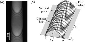
Alekseenko et al. (Reference Alekseenko, Markovich and Shtork1996) performed the first detailed experimental study of the wave motion of a rectilinear rivulet for the case of liquid flow along the lower outer wall of an inclined tube. The region of existence of stationary periodic waves was determined. The waves were shown to always have a three-dimensional horseshoe shape, and their profile (in the longitudinal section) can both match the case of the waves on the falling liquid films and take on other forms. Later, instantaneous velocity fields in the wave rivulet on an inclined tube were measured (Alekseenko et al. Reference Alekseenko, Antipin, Bobylev and Markovich2007). The instantaneous axial velocity profile was found to vary slightly in relation to self-similar parabolic profile, that may serve as justification for the application of the integral method of Kapitza–Shkadov to wave rivulets. Previously, this method was successfully applied to the wavy liquid films (Alekseenko, Nakoryakov & Pokusaev Reference Alekseenko, Nakoryakov and Pokusaev1985). A feature of a rivulet flow along the inclined cylinder is that the flow is always rectilinear; therefore, it is relatively easy to investigate this flow both experimentally and theoretically. It is considerably more difficult to observe the rectilinear rivulet flow over a vertical or inclined plane due to the tendency of the flow to meander. Alekseenko et al. (Reference Alekseenko, Bobylev, Guzanov, Markovich and Kharlamov2010) were the only researchers to present the results of experimental investigations on large-amplitude, periodic, stationary waves on a rectilinear rivulet flowing down a vertical wall. The waves are shown to be predominantly three-dimensional (see figure 1 a), and the patterns of their motion depend strongly on the magnitude of the contact angle of wetting. The results of this experiment are discussed in § 3.1 in more detail to validate the theoretical model and for comparison with the calculation.
(a) Visualization of wavy rivulet flow using the LIF technique (experimental set-up of Alekseenko et al. (Reference Alekseenko, Bobylev, Guzanov, Markovich and Kharlamov2010), forcing frequency: 17 Hz) and (b) rivulet flow diagram.

The analysis of data from the literature demonstrates that there is a limited number of theoretical works that have examined the linear stability of rectilinear rivulets flowing downward over a narrow range of conditions (small Reynolds numbers and plane modes of perturbations only) and without comparison with experiments. Examples of calculations of nonlinear waves in the literature are lacking.
The objective of this paper is to attempt to theoretically describe nonlinear, developed, periodic waves on a vertically flowing rivulet. The spatiotemporal evolution of perturbations was considered in three-dimensional formulations. The Kapitza–Shkadov integral method was applied since it was well proven in the study of both two- and three-dimensional nonlinear waves in falling liquid films over a wide range of Reynolds numbers. The peculiarity of this work is the use of experimental data, particularly the condition of constancy of the rivulet width (fixed contact line), for validation of the theoretical approach. Therefore, there is no need to vary the boundary conditions at the contact line due to the lack of appropriate knowledge. The calculations are performed only for the conditions implemented in the experiment. Comparisons of calculated and experimental data were performed. Conclusions regarding the possible application of the developed theoretical method to a description of wavy rivulets were drawn.
2. Theoretical model
Let us consider a thin liquid layer flow over a vertical flat plate as a rivulet of constant width
 $2b$
. We introduce a Cartesian coordinate system
 $Oxyz$
with the
 $Ox$
-axis directed along gravity and the
 $Oy$
-axis directed along the normal to the plate (figure 1
b). Let us assume that the layer thickness
 $h$
is substantially smaller than the rivulet semi-width
 $b$
and the wavelength
 ${\it\lambda}$
(long-wave approximation). All of these assumptions are in good agreement with experimental observations (Alekseenko et al.
Reference Alekseenko, Bobylev, Guzanov, Markovich and Kharlamov2010, see § 3.1).
As a first approximation with respect to the small parameters
 ${\it\varepsilon}_{{\it\lambda}}=h/{\it\lambda}$
,
 ${\it\varepsilon}_{b}=h/b$
, the waves in a liquid layer may be described by the integral boundary layer (IBL) model of Demekhin & Shkadov (Reference Demekhin and Shkadov1984), which was developed for three-dimensional long waves in a falling liquid film. The IBL model, which is called the Kapitza–Shkadov model in the literature, is the main theoretical approach for simulation of two-dimensional nonlinear waves in flowing liquid films at moderate Reynolds numbers (Alekseenko et al.
Reference Alekseenko, Nakoryakov and Pokusaev1985; Chang & Demekhin Reference Chang and Demekhin2002; Kalliadasis et al.
Reference Kalliadasis, Ruyer-Quil, Scheid and Velarde2012). This model is also well proven in the case of three-dimensional wave motion. This is confirmed by the calculations of Demekhin, Kalaidin & Selin (Reference Demekhin, Kalaidin and Selin2010) of 3D solitons in liquid films, which are in good agreement with the experiments of Alekseenko et al. (Reference Alekseenko, Antipin, Guzanov, Kharlamov and Markovich2005) performed at Reynolds numbers within the range of
 $1$
–
 $5$
. The characteristic scales of velocity and dimensions as well as wave forms on the liquid film and rivulet are similar; therefore, quite adequate application of the IBL model to describe the wave motion of rivulets is expected. The use of lubrication theory, which is valid for small Reynolds numbers and is commonly used in the literature to describe rivulets, is not acceptable in this case because the developed waves on rivulets are observed at sufficiently high values of Reynolds numbers equal to
 $10$
–
 $50$
(Alekseenko et al.
Reference Alekseenko, Markovich and Shtork1996, Reference Alekseenko, Bobylev, Guzanov, Markovich and Kharlamov2010).
Within the IBL model of Demekhin & Shkadov (Reference Demekhin and Shkadov1984), the corresponding momentum and mass balance equations in dimensionless variables are as follows:
 $$\begin{eqnarray}\displaystyle & \displaystyle \frac{\partial q}{\partial t}+\frac{6}{5}\left(\frac{\partial }{\partial x}\frac{q^{2}}{h}+\frac{\partial }{\partial z}\frac{qm}{h}\right)=\frac{3}{\mathit{Re}_{m}}\left(h-\frac{q}{h^{2}}\right)+hWe\frac{\partial {\rm\Delta}h}{\partial x}, & \displaystyle\end{eqnarray}$$
 $$\begin{eqnarray}\displaystyle & \displaystyle \frac{\partial m}{\partial t}+\frac{6}{5}\left(\frac{\partial }{\partial z}\frac{m^{2}}{h}+\frac{\partial }{\partial x}\frac{qm}{h}\right)=hWe\frac{\partial {\rm\Delta}h}{\partial z}-\frac{3}{\mathit{Re}_{m}}\frac{m}{h^{2}}, & \displaystyle\end{eqnarray}$$
 $$\begin{eqnarray}\displaystyle & \displaystyle \frac{\partial h}{\partial t}+\frac{\partial q}{\partial x}+\frac{\partial m}{\partial z}=0. & \displaystyle\end{eqnarray}$$
 $q(x,z,t)=\int _{0}^{h}u\,\text{d}y$
and
 $m(x,z,t)=\int _{0}^{h}w\,\text{d}y$
are the liquid flow rates per unit width along the Ox- and Oz-axes, respectively. Equations (2.1a
) and (2.1b
) are deduced from the Navier–Stokes equations in the boundary-layer approximation using self-similar profile of the velocity:
 $u/u_{s}=2{\it\eta}-{\it\eta}^{2}$
,
 $w/w_{s}=2{\it\eta}-{\it\eta}^{2}$
, where
 ${\it\eta}=y/h$
,
 $u$
and
 $w$
are the components of velocity, and the subscript
 $s$
denotes the value at a liquid surface. In (2.1a
) and (2.1b
),
 ${\rm\Delta}h=\partial ^{2}h/\partial x^{2}+\partial ^{2}h/\partial z^{2}$
is the curvature of the liquid surface,
 $\mathit{Re}_{m}=gh_{0}^{3}/3{\it\nu}^{2}$
is the Reynolds number,
 $We=(3\mathit{Fi}/\mathit{Re}_{m}^{5})^{1/3}$
is the Weber number,
 $\mathit{Fi}={\it\sigma}^{3}/{\it\rho}^{3}g{\it\nu}^{4}$
is the film number (or the Kapitza number),
 ${\it\sigma}$
is the surface tension,
 ${\it\rho}$
is the density and
 ${\it\nu}$
is the kinematic viscosity of fluid. We choose the unperturbed film thickness
 $h_{0}$
at the symmetry axis of the rivulet as the scale and introduce the scales of velocity
 $gh_{0}^{2}/3{\it\nu}$
, time
 $3{\it\nu}/gh_{0}$
and flow rate
 $gh_{0}^{3}/3{\it\nu}$
.
It is assumed that on the plate the no-slip condition is valid:
 $u=v=w=0$
, where
 $v$
is the velocity component transverse to the wall. In addition, on the liquid surface, we have the kinematic condition
 $$\begin{eqnarray}\frac{\partial h}{\partial t}+u_{s}\frac{\partial h}{\partial x}+w_{s}\frac{\partial h}{\partial z}=v_{s}\end{eqnarray}$$
and the dynamic conditions
 $$\begin{eqnarray}p=p_{g}-{\it\sigma}(\partial ^{2}h/\partial x^{2}+\partial ^{2}h/\partial z^{2}),\quad \partial u/\partial y=0,\quad \partial w/\partial y=0,\end{eqnarray}$$
where
 $p_{g}$
is gas pressure above the liquid surface. The Navier–Stokes equation for the
 $v$
component of the velocity in the boundary layer approximation has the form
 $\partial p/\partial y=0$
, which indicates a constant pressure across the layer of liquid. Hence, considering the dynamic conditions (2.3) for normal stress the pressure in the liquid is determined only by surface tension:
 $p=p_{g}-{\it\sigma}(\partial ^{2}h/\partial x^{2}+\partial ^{2}h/\partial z^{2})$
. With regard to the rivulet flow, equation (2.1) must be supplemented by the boundary conditions at the contact line (fixed contact line)
 $$\begin{eqnarray}h(x,b,t)=q(x,b,t)=m(x,b,t)=0\end{eqnarray}$$
and the following symmetry conditions:
 $m|_{z=0}=0$
,
 $\partial h/\partial z|_{z=0}=\partial q/\partial z|_{z=0}=0$
. For the unperturbed rivulet flow, we obtain from (2.1a
) and (2.1b
)
 $$\begin{eqnarray}h=h_{st}=1-z^{2}/b^{2},\quad q=q_{st}=h_{st}^{3}(z),\quad m=0.\end{eqnarray}$$
It follows from the first formula in (2.5) that the contact wetting angle is
 ${\it\theta}=\arctan (2h_{0}/b)$
(see figure 1
b). This means that there is no need to introduce a contact wetting angle in the case of a constant rivulet width. This angle is determined by the parameter
 $h_{0}/b$
.
From (2.5), we can calculate the liquid flow rate in unperturbed rivulet (in dimensional form)
 $$\begin{eqnarray}Q_{0}=\frac{gh_{0}^{3}}{3{\it\nu}}\int _{-b}^{b}q_{st}(z)\,\text{d}z=\frac{2gh_{0}^{3}}{3{\it\nu}}\int _{0}^{b}\left(1-\frac{z^{2}}{b^{2}}\right)^{3}\,\text{d}z=\frac{32gh_{0}^{3}}{105{\it\nu}}.\end{eqnarray}$$
Equation (2.6) exactly coincides with the results of Towell & Rothfeld (Reference Towell and Rothfeld1966) and Duffy & Moffatt (Reference Duffy and Moffatt1995) for thin rivulet flows on vertical plate and with the experimental data of Alekseenko et al. (Reference Alekseenko, Bobylev, Guzanov, Markovich and Kharlamov2010). For a liquid film with thickness
 $h_{0}$
, the flow rate in a strip of width
 $2b$
is
 $$\begin{eqnarray}Q_{film}=\frac{2gh_{0}^{3}b}{3{\it\nu}}.\end{eqnarray}$$
Equations (2.6) and (2.7) demonstrate that
 $Q_{0}=16Q_{film}/35$
, i.e. the flow rate of the liquid in a rivulet with thickness
 $h_{0}$
is approximately half of that in a film of the same thickness. The area of the rivulet cross-section considering the first expression in (2.5), is
 $$\begin{eqnarray}S_{0}=\int _{-b}^{b}h\,\text{d}z=\frac{4}{3}h_{0}b.\end{eqnarray}$$
Then, from (2.6) and (2.8), for the velocity averaged over the cross-section, we obtain
 $$\begin{eqnarray}u_{0}=\frac{Q_{0}}{S_{0}}=\frac{8gh_{0}^{2}}{35{\it\nu}}.\end{eqnarray}$$
Assuming that (2.6) and (2.8) remain valid for the local values at the propagation of long-wave plane perturbations of small amplitude in the rivulet, it is easy to obtain the expression for the velocity of such perturbations. Integrating equation (2.1c ) over the rivulet width and considering (2.4), we have (in dimensional form)
 $$\begin{eqnarray}\frac{\partial S}{\partial t}+\frac{\partial Q}{\partial x}=0,\end{eqnarray}$$
where the local values of flow rate
 $Q$
and cross-section area
 $S$
are related to the local thickness
 $H$
on the rivulet axis by (2.6) and (2.8). Substitution of these relations into (2.10) yields
 $$\begin{eqnarray}\frac{\partial H}{\partial t}+\frac{24gH^{2}}{35{\it\nu}}\frac{\partial H}{\partial x}=0.\end{eqnarray}$$
Assuming that
 $H=h_{0}+h^{\prime }(x,t)$
, where
 $h^{\prime }$
is a small perturbation, we obtain from (2.11) in the linear approximation
 $$\begin{eqnarray}\frac{\partial h^{\prime }}{\partial t}+C_{kin}\frac{\partial h^{\prime }}{\partial x}=0.\end{eqnarray}$$
This equation describes the propagation of a so-called kinematic wave with velocity
 $$\begin{eqnarray}C_{kin}=\frac{24gh_{0}^{2}}{35{\it\nu}}=3u_{0}.\end{eqnarray}$$
The kinematic wave velocity in the rivulet reduced to the liquid velocity averaged over the cross-section is equal to 3, which exactly coincides with the respective value for the kinematic wave in the falling liquid film (Alekseenko et al. Reference Alekseenko, Nakoryakov and Pokusaev1985). This is not surprising because the same parabolic velocity profile is used for both the liquid film and rivulet. In addition equation (2.13) exactly coincides with the limit velocity of infinitely long waves in rivulets, which was obtained by Weiland & Davis (Reference Weiland and Davis1981) and Young & Davis (Reference Young and Davis1987) for the same case of a fixed contact line. The velocity of the kinematic wave is a characteristic velocity of two-dimensional waves and is used as a reference value for comparison.
Let us consider another problem that is relevant to the studied rivulet flow regimes and that also provides the expression for the kinematic wave velocity. Let the perturbation has the form of a ‘positive step’, propagating downstream with constant velocity
 $C$
. This is the analogue of a shock wave in gas dynamics. Before the ‘step’, a smooth equilibrium rivulet is characterised by a flow rate
 $Q_{1}$
, a cross-sectional area
 $S_{1}$
and a maximum thickness
 $h_{1}$
, and behind the ‘step’ the corresponding quantities are
 $Q_{2}$
,
 $S_{2}$
and
 $h_{2}$
. Beyond the ‘step’ all of these parameters are larger than before the ‘step’, and the rivulet width
 $2b$
is accepted to be equal. The latter assumption seems questionable for a rivulet flow with stepwise varying parameters. However, for a sufficiently small increase in the flow rate, as well as when a variation in the parameters occurs along a sufficiently short length of the rivulet, the assumption of constant rivulet width can be considered quite acceptable. Then, in the wave related system, we can write the flow rate balance as follows:
 $$\begin{eqnarray}S_{2}C-Q_{2}=S_{1}C-Q_{1}.\end{eqnarray}$$
From this equation, considering the relations for the equilibrium values of the flow rate and cross-section area, we obtain the expression for the velocity
 $C$
 $$\begin{eqnarray}C=\frac{Q_{2}-Q_{1}}{S_{2}-S_{1}}=\frac{8gh_{2}^{2}}{35{\it\nu}}(1+n+n^{2}),\end{eqnarray}$$
where the thickness ratio is
 $n=h_{1}/h_{2}<1$
. For arbitrary values of
 $n<1$
, equation (2.15) describes the propagation velocity of a ‘step’ of finite amplitude, and the spatial structure of the ‘step’ edge is not important. In the case of relatively small disturbances, i.e.
 ${\rm\Delta}h\equiv h_{2}-h_{1}\ll h_{1}$
, at a fixed thickness
 $h_{1}$
we obtain from (2.15) linear relationship between
 $C$
and
 ${\rm\Delta}h$
:
 $$\begin{eqnarray}C=\frac{24gh_{1}^{2}}{35{\it\nu}}\left(1+\frac{{\rm\Delta}h}{h_{1}}\right).\end{eqnarray}$$
In the limit
 ${\rm\Delta}h\rightarrow 0$
we get the velocity of a kinematic wave (2.13). In contrast, at a large disturbance
 $h_{2}\gg h_{1}~(n\rightarrow 0)$
, we obtain a quadratic relationship between the wave velocity and local rivulet thickness:
 $C=8gh_{2}^{2}/35{\it\nu}$
.
3. Calculations and comparison with the experiments
Wave regimes of the rivulet flow are obtained by numerically solving (2.1) using the finite difference method and an implicit scheme. The numerical algorithms use the conditions at the contact line (2.4), and (2.5) serve as the initial conditions. Waves were generated at the inlet of the model domain, where sinusoidal oscillations of the flow rate were established as follows:
 $$\begin{eqnarray}q(0,z,t)=q_{st}[1+A_{q}\sin (2{\rm\pi}ft)].\end{eqnarray}$$
Here,
 $A_{q}$
and
 $f$
are the amplitude and forcing frequency, respectively. All calculations were performed for the experimental conditions of Alekseenko et al. (Reference Alekseenko, Bobylev, Guzanov, Markovich and Kharlamov2010). The results of this work that are necessary for comparison are described below.
3.1. Main results of the experiment of Alekseenko et al. (Reference Alekseenko, Bobylev, Guzanov, Markovich and Kharlamov2010)
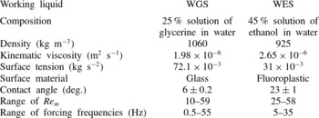
The experiment focused on steady periodic waves in rectilinear rivulets flowing down a vertical wall. The main difficulty was forming a rectilinear rivulet due to the rivulet’s tendency to meander and other phenomena. It was possible to select only two pairs of ‘liquid’–‘solid’ when the rectilinear rivulet with constant width was formed. In the first variant, the flow of 25 % water–glycerine solution (WGS) over a glass plate with a clean uniform surface was studied. The contact wetting angle
 ${\it\theta}_{0}$
was determined from an experimentally measured cross-sectional profile of a smooth rivulet and was equal to
 $6\pm 0.2^{\circ }$
. In the second variant, a 45 % solution of ethanol in water (WES) was used as the working liquid. The working section was a plate that was covered with a homogeneous thin fluoroplastic film. As a result, a poorly wettable surface with a contact angle equal to
 $23\pm 1^{\circ }$
for the WES was produced. All of the main properties of the liquids, as well as the conditions of the experiment, are shown in table 1.
Conditions of experiments of Alekseenko et al. (Reference Alekseenko, Bobylev, Guzanov, Markovich and Kharlamov2010).

To produce the rivulet flow, the liquid was supplied on the plate through a rectangular slit with a gap of 2.5 mm and an adjustable length of 1–10 mm. A rather large area of hydrodynamic stabilization compared with the case of liquid film flow was observed. Therefore, the measurements were performed at sufficiently large distances from the entrance at
 $x>30~\text{cm}$
, when a rivulet with unchanged characteristics was formed. Unlike film flows, the natural waves on the rivulet were not observed under the conditions of this experiment. Therefore, the wave generation on the rivulet was studied by applying external perturbations, such as periodic pulsations of the liquid flow rate (see a similar approach for liquid films in Alekseenko et al. (Reference Alekseenko, Nakoryakov and Pokusaev1985)). As a result of forcing, regular periodic waves were formed at some distance from the entrance. The region of existence of stationary periodic waves, which depends only on the Reynolds number and forcing frequency at given values of the wetting contact angle and liquid properties, was determined. It follows from the experiment that the wave patterns differ significantly for variants with different wetting contact angles (6° and 23°), which were named ‘small’ and ‘large’ wetting contact angles, respectively. At a ‘small’ contact angle, i.e.
 ${\it\theta}_{0}=6^{\circ }$
, the rivulet can be considered thin as it is assumed in the lubrication approximation. For example, if
 $\mathit{Re}_{m}=25$
, the rivulet thickness would be
 $h_{0}=0.31~\text{mm}$
at a width of 20 mm. The steady-state waves exhibit a pronounced three-dimensional horseshoe shape (see figure 1
a). For small forcing frequencies, these waves are similar to the ones on liquid films. At a ‘large’ contact angle, i.e.
 ${\it\theta}_{0}=23^{\circ }$
, the transverse rivulet profile is substantially more convex (for
 $\mathit{Re}_{m}=25$
, the rivulet thickness would be
 $h_{0}=0.38~\text{mm}$
at a width of approximately 4 mm). However, the form of waves in the projection on the plate is close to two-dimensional. The experimentally observed images of waves are shown in subsequent figures during the comparison with theoretical calculations (figures 11–14). In this experiment, it was not possible to find other pairs of ‘liquid’–‘solid’ that would enable the study of wave motion of rectilinear rivulet with wave patterns, transitional between the cases of ‘small’ and ‘large’ contact angles.
The local rivulet thickness was measured using laser-induced fluorescence (LIF) with an accuracy of no less than 4 % in the larger part of the rivulet width. Near the contact line, where the thickness of the liquid layer tends to zero, the absolute accuracy was several micrometres, but the relative error was quite large. Therefore, the contact angle and position of the contact line were determined in the experiments through extrapolation of the rivulet form in the region, where its thickness was no less than
 $20$
–
 $30~{\rm\mu}\text{m}$
. Consequently, the rivulet width remained constant to an accuracy of 0.2 mm. For the investigated flow conditions, the rivulet width remained constant with the specified accuracy over the entire measurement area, which had a length of 9.5 cm. The experimentally confirmed point of the constant rivulet width (fixed contact line) is used as a basic assumption when developing the above theoretical model of rivulet wave motion.
3.2. Linear waves
In the numerical simulations, similar to the experiment, nonlinear steady-state waves were formed as a result of the spatiotemporal evolution of the initial sinusoidal disturbances of the liquid flow rate governed by (3.1). At values of
 $A_{q}<0.01$
, the amplitude of arising waves is sufficiently small that the waves can be considered linear. To study the dispersion properties of the linear perturbations and provide further comparison with the regularities of nonlinear wave propagation, the evolution of perturbations in the linear region was numerically simulated (for only a few special cases). The liquid properties and flow parameters were chosen using the values listed in table 1, and the rivulet half-width
 $b$
required for the calculation was assumed to be equal to
 $1\times 10^{-2}~\text{m}$
for WGS and
 $2\times 10^{-3}~\text{m}$
for WES based on the experimental data obtained at
 $\mathit{Re}_{m}=25$
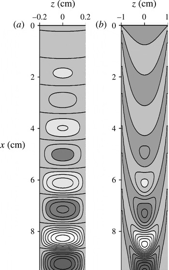
. Figure 2 reveals the calculated results for linear waves in (a) the WES rivulet and (b) the WGS rivulet at
 $f=15~\text{Hz}$
,
 $A_{q}=0.01$
and
 $\mathit{Re}_{m}=25$
. The perturbation of the rivulet surface
 ${\it\delta}h=h(x,z,t)-h_{st}(z)$
is shown in the form of contours
 ${\it\delta}h=\text{const.}$
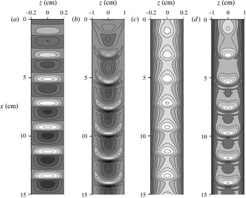
at fixed times. The waves have the form of alternating hills and troughs. Figure 2(a) shows that for the WES rivulet, the wave crests are nearly straight. Thus, the perturbations are nearly two-dimensional even though the waveform is three-dimensional. Such perturbations may be considered within theories of plane waves. In the case of the WGS rivulet (figure 2
b), the wave crests are horseshoe shaped, i.e. the waves are essentially three-dimensional. Nearly two-dimensional waves in the WES rivulet and three-dimensional waves in the WGS rivulet are formed in the investigated frequency range. Approaches to stability analysis for plane waves based on lubrication theory and presented in the literature are not applicable here due to the use of large Reynolds numbers and the predominantly three-dimensional nature of waves (in the case of the WGS rivulet).
Linear waves in (a) the WES rivulet and in (b) the WGS rivulet at
 $f=15~\text{Hz}$
,
 $\mathit{Re}_{m}=25$
. The disturbances of the rivulet surface are shown as contours
 ${\it\delta}h=\text{const.}$
with a 0.05 mm step. Light areas are hills and dark areas are troughs.

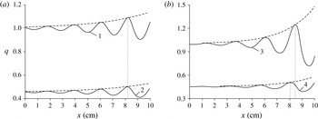
Increasing amplitude of linear waves at 15 Hz in (a) the WES and (b) the WGS rivulets. Curves 1 and 3 show the distributions
 $q(x)$
at
 $z=0$
, and curves 2 and 4 show the distributions
 $q(x)$
at
 $z/b=0.48$
. The dashed lines are approximations of envelopes in the form
 $q=q_{st}(z)[1+A\exp ({\it\beta}x)]$
. Here,
 ${\it\beta}=0.26$
for WES and
 ${\it\beta}=0.439$
for WGS;
 $A$
for curves 1–4 are equal to 0.012, 0.0104, 0.006 and 0.0034.

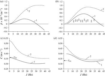
Dispersion dependencies (curves 1) for linear waves in (a,c) the WES rivulet and in (b,d) the WGS rivulet. Curves 2 are the corresponding dependencies for two-dimensional waves in the film, which are calculated using linear theory, and open circles are experimental data.

The development of linear perturbations is accompanied by the exponential growth (or decay) of the amplitude with increasing distance (at
 $z=0$
) based on
 $$\begin{eqnarray}q(x,0,t)=1+A\sin (k[x-Ct])\exp ({\it\beta}x).\end{eqnarray}$$
Here,
 $k=2{\rm\pi}h_{0}/{\it\lambda}$
is the wavenumber,
 ${\it\beta}$
is the spatial increment and
 $C$
is the phase velocity. Both
 $C$
and
 ${\it\beta}$
depend on the forcing frequency. Disturbances grow at
 ${\it\beta}>0$
, whereas they decay at
 ${\it\beta}<0$
. To confirm the linear nature of the considered perturbations, the growth in the amplitude of developing waves of 15 Hz in the WGS rivulet at
 $A_{q}=0.005$
and in the WES rivulet at
 $A_{q}=0.01$
is shown in figure 3. To control the changes in curvature of the wave crests during their development, the calculated distributions
 $q(x)$
are presented at both
 $z=0$
and
 $z/b=0.48$
for a fixed point in time. The dashed lines are the approximations of envelopes in the form
 $q=q_{st}(z)[1+A\exp ({\it\beta}x)]$
at
 ${\it\beta}=0.26$
for the WES and
 ${\it\beta}=0.439$
for the WGS. Figure 3(a,b) illustrate that the distributions
 $q(x)$
are in good agreement with (3.2). According to figure 3(a) for the WES rivulet, the envelopes of the curves
 $q(x)$
for different
 $z$
are described by one value,
 ${\it\beta}=0.26$
, and the phases of the oscillations coincide, i.e. the waves are two-dimensional. For the WGS rivulet, the envelopes of the curves
 $q(x)$
in figure 3(b) are described by
 ${\it\beta}=0.439$
only when
 $x>3~\text{cm}$
, and when
 $x<3~\text{cm}$
, three-dimensional waves are being formed. In addition, there is a phase shift between the oscillations of the curves 3 and 4 at
 $x>3~\text{cm}$
due to the three-dimensional nature of waves. A constant phase shift and the same value of
 ${\it\beta}$
for the envelopes of the curves in figure 3(b) mean that at
 $x>3~\text{cm}$
, the curvature of the wave crests remains constant.
The dispersion dependencies
 $C(f)$
and
 ${\it\beta}(f)$
were calculated using the results of the simulation of the linear waves in their exponential growth region. The wavelength was calculated as the distance between adjacent peaks at
 $z=0$
, whereas the phase velocity was determined by the displacement of the peaks. The spatial increment was computed by the ratio of the flow rate oscillation amplitudes
 $A_{1}$
and
 $A_{2}$
for two values of the coordinates
 $x_{1}$
and
 $x_{2}$
using the formula
 ${\it\beta}=\ln (A_{2}/A_{1})/(x_{2}-x_{1})$
. Figure 4 shows the spatial increment (a,b) and phase velocity (c,d) of linear waves in the WES and WGS rivulets as a function of the frequency at
 $\mathit{Re}_{m}=25$
. For comparison, the corresponding curves for two-dimensional waves in the film are also shown, which are calculated by linear theory for the same value of
 $\mathit{Re}_{m}$
. Figure 4 clearly shows that the curves
 $C(f)$
and
 ${\it\beta}(f)$
for the rivulet flow are qualitatively similar to the corresponding curves for the film flow. The phase velocity first decreases with increasing frequency, passing through a minimum, and subsequently begins to rise. However, the wave velocity in the rivulet is substantially less than the velocity of two-dimensional waves in the film within the investigated frequency range. The spatial increment for the rivulet flow is significantly lower, and the instability frequency range is essentially narrower than that for a film flow. Intuitively, one would expect that the values of the increment for travelling disturbances on a rivulet should be smaller compared with the uniform liquid film due to the additional dissipation in the vicinity of the contact line. In general, for the WGS rivulet curves,
 ${\it\beta}(f)$
and
 $C(f)$
are higher and closer to the corresponding ‘film’ curves than for the WES rivulet, which is not surprising. Because the parameter
 $h_{0}/b$
for the WGS rivulet is approximately five times smaller than that for the WES rivulet, it is natural to expect that the waves in the WGS rivulet are more consistent with waves in liquid films. The most rapidly growing waves for falling liquid films occur in practice, i.e. waves with a frequency corresponding to the maximum value of the increment. In the case of a rivulet, the increments are significantly smaller compared with the film flow, which explains the absence of natural waves in rather short rivulets in the experiment. The arrow in figure 4(c,d) indicates the velocity of the kinematic wave
 $C_{kin}$
, which is determined by (2.13); this equation is valid for two-dimensional, infinitely long waves. For the WES rivulet, the value
 $C_{kin}=0.361~\text{m}~\text{s}^{-1}$
is in good agreement with the calculated dependence
 $C(f)$
at
 $f\rightarrow 0$
. This is well explained by the fact that waves in the WES rivulet are nearly two-dimensional, i.e. they meet the conditions under which (2.13) is obtained. For the WGS rivulet, the value
 $C_{kin}=0.329~\text{m}~\text{s}^{-1}$
is significantly lower than the respective values on the calculated curve. Low-frequency waves in the WGS rivulet are essentially three-dimensional; therefore, (2.13) may be not applicable to them. The value of the wave velocity in the WGS rivulet at
 $f\rightarrow 0$
is located between
 $C_{kin}$
and the corresponding value for the film. For two-dimensional linear waves on the liquid film (dashed lines in figure 4), the values of the kinematic wave velocity exactly coincide with those of the velocity on the dispersion curves at
 $f\rightarrow 0$
.
In the experiment of Alekseenko et al. (Reference Alekseenko, Bobylev, Guzanov, Markovich and Kharlamov2010), linear waves in the region of their occurrence were not studied in detail. However, it was possible to perform an evaluation based on a small set of available experimental data for developing waves in a WGS rivulet. According to the results from processing the experimental images of the surface wave, which correspond to two instants in time, we calculated the wave increment and wave velocity. Figure 4(b) also shows a comparison of the calculated values of the wave increment for the WGS rivulet with the results of the processed data. Figure 4(b) clearly shows that the experimental values of the increment obtained in the range of
 $12$
–
 $35~\text{Hz}$
are significantly lower than the calculated values. Because the experimental conditions of disturbance waves differ considerably from condition (3.1) used in the calculations and because they apparently correspond to the area of hydrodynamically unsteady flows with unknown velocity profiles, it is difficult to expect good agreement. The experimental values of the developing wave velocity have considerable scatter. On average, they are approximately
 $1.5$
–
 $1.7$
times higher than the calculated values in the investigated frequency range. In addition to unsteady flow, one possible explanation for the discrepancies between the calculations and experiment for the wave velocity may be related to the hypothesis of self-similar velocity profiles used in the theoretical model. Therefore, without further experimental studies of the hydrodynamic patterns of rivulets, especially in the area of flow development, it is difficult to draw conclusions about the agreement between the theory and experiments. The validity of the theoretical model, at least for two-dimensional waves, is confirmed by the agreement with kinematic waves and the calculations of Weiland & Davis (Reference Weiland and Davis1981) and Young & Davis (Reference Young and Davis1987) for extremely long waves.
3.3. Nonlinear waves
To consider nonlinear waves, the amplitude
 $A_{q}$
of the flow rate pulsations was varied within the range of
 $0.1$
–
 $0.3$
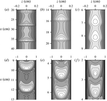
. With such large initial amplitudes, waves lose their sinusoidal shape close to the inlet. If the forcing frequency is within the range of instability, the perturbations grow with distance and form steady travelling nonlinear waves at some distance from the inlet. Figure 5 shows the development of nonlinear waves at a frequency of 15 Hz in the WES and WGS rivulets at the same value of
 $\mathit{Re}_{m}=25$
. Figure 5(a,b) show the wave surface of the rivulet in the form of contours
 ${\it\delta}h=\text{const.}$
, as in figure 2(a,b), where the evolution of linear perturbations under the same conditions is presented. In the case of large-amplitude perturbations, it is more convenient to analyse wave patterns in the form of isothickness contours,
 $h=\text{const.}$
(figures 5
c,d and 8). Figure 5(c,d) demonstrate that the wave flow becomes steady at a distance of
 $3$
–
 $5$
wavelengths. For the WES rivulet, the waves are nearly two-dimensional (in relation to the wave crest), whereas the waves in the WGS rivulet exhibit a characteristic horseshoe shape, i.e. they are significantly three-dimensional. The distinction between WES and WGS is apparently due to the difference in the parameter
 $h_{0}/b$
, but this is not obvious or predictable. If we compare the appropriate patterns of linear (figure 2
a,b) and nonlinear (figure 5
a,b) waves, we can observe essential differences both in terms of the shape of the waves and the length of their development zone.
The 15 Hz nonlinear waves in (a,c) the WES rivulet and (b,d) the WGS rivulet at
 $\mathit{Re}_{m}=25$
. The wave surface of the rivulet is shown as contours
 ${\it\delta}h=\text{const.}$
with the step of (a) 0.02 mm, (b) 0.025 mm and (c,d) isothickness contours
 $h=\text{const.}$
with 0.05 mm step. Light areas are hills and dark areas are troughs.

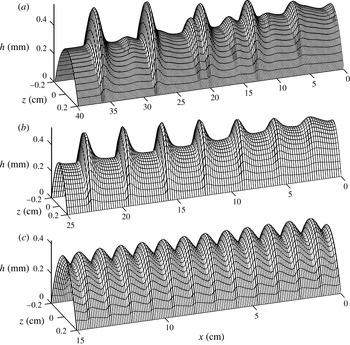
Calculated 3D surface of developing waves in WES rivulet at
 $\mathit{Re}_{m}=25$
and different values of the forcing frequency: (a) 5 Hz; (b) 10 Hz; (c) 25 Hz.

Figure 6 shows a 3D surface of developing waves in the WES rivulet at
 $b=2\times 10^{-3}~\text{m}$
and
 $\mathit{Re}_{m}=25$
for different forcing frequencies. The same data are presented in figure 8(a–c) in additional detail in the form of isothickness contours
 $h=\text{const.}$
away from the inlet when the waves are essentially steady. The scales on the
 $x$
-axis are different for patterns with different frequencies. Figures 6(a,b) and 8(a,b) clearly show that the waves have the shape of a blade with a steep leading edge and flat rear slope. At a low forcing frequency of 5 Hz, an interesting feature is observed for developing waves (see figure 6
a): intermediate peaks of smaller amplitude are formed between main large peaks (which correspond to the forcing frequency
 $f$
). At that, they interact with each other because of the difference in propagation velocities of the main and intermediate peaks. As a result of this interaction, the main peaks absorb the intermediate peaks. Argyriadi, Serifi & Bontozoglou (Reference Argyriadi, Serifi and Bontozoglou2004) experimentally and theoretically investigated the effect of intermediate peaks for the case of two-dimensional waves in a liquid film. Such perturbations were called parasitic pulses. The appearance of parasitic pulses was observed on the rear slope of large-amplitude waves at forcing frequencies below a certain limiting value. The profile of a high-frequency wave (see figures 6
c and 8
c) is similar to a sinusoid but with a steeper slope at the edge. The waves immediately become steady at the inlet.
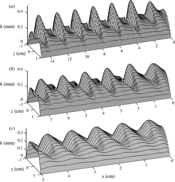
Calculated 3D surface of developing waves in WGS rivulet at
 $\mathit{Re}_{m}=25$
and different values of the forcing frequency: (a) 15 Hz; (b) 25 Hz; (c) 30 Hz.

Developed nonlinear waves in (a–c) the WES rivulet and (d–f) the WGS rivulet at
 $\mathit{Re}_{m}=25$
. The rivulet surface is depicted using isothickness contours
 $h=\text{const.}$
with 0.05 mm step. Light areas are hills and dark areas are troughs.

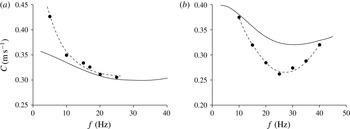
Velocity of developed nonlinear waves (full circles) in (a) the WES rivulet and (b) the WGS rivulet at
 $\mathit{Re}_{m}=25$
as a function of the forcing frequency. Solid lines show corresponding dependencies for linear waves and dashed lines show approximations of calculated data.

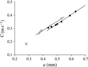
Velocity of the developed nonlinear waves in the WES and WGS rivulet at
 $\mathit{Re}_{m}=25$
as a function of the wave amplitude. Full circles represent the WES (frequency of 5, 7, 10, 15, 17, 20 and 25 Hz), open circles represent the WGS (frequency of 10, 15, 20, 25 and 30 Hz). The square symbol denotes the data for the step-wise wave (WGS,
 $\mathit{Re}_{m}=10$
,
 $f=1~\text{Hz}$
). Straight lines are approximations of calculated data.

The development of three-dimensional waves on the surface of the WGS rivulet at
 $b=1\times 10^{-2}~\text{m}$
and
 $\mathit{Re}_{m}=25$
for different forcing frequencies is shown in figures 7 and 8(d–f), respectively. These figures illustrate that the developed wave has a high horseshoe-shaped amplitude peak with a steep leading edge and gentle rear slope. Ahead of the main peak, capillary ripples are formed (see figures 7
a,b and 8
d,e); they gradually disappear with increasing frequency (see figures 7
c and 8
f). The amplitude of the developed waves, similar to the WES rivulet, depends on the forcing frequency. Figure 8, in which the data from figures 6 and 7 are depicted as isothickness contours
 $h=\text{const.}$
, provides a clear comparison of the structure of the wave rivulet surface as a function of both the forcing frequency and liquid properties (for two cases, which vary greatly in the film number Fi; see table 1).
The wave characteristics of steady nonlinear waves on the rivulet are presented in figures 9 and 10. Figure 9(a,b) show the dependence of the nonlinear waves’ velocity on the forcing frequency in comparison with calculations for linear perturbations. The figures demonstrate that the velocity of the nonlinear waves can exceed the velocity of linear waves of the same frequency, which is the case for the WES rivulet, but may be lower than the velocity of linear waves observed for the WGS rivulet. With a high-frequency perturbation, in the case of the WES rivulet, the velocity of the nonlinear waves coincides with the linear perturbation velocity, which is typical for two-dimensional waves in liquid films. Another notable regularity of stationary waves is a linear relationship between wave velocity and amplitude. This regularity was found experimentally both for two-dimensional waves in a liquid film (Alekseenko et al.
Reference Alekseenko, Nakoryakov and Pokusaev1985) and for three-dimensional waves in rivulets flowing along the lower side of an inclined cylinder (Alekseenko et al.
Reference Alekseenko, Markovich and Shtork1996). The amplitude can be defined as the maximum thickness of the liquid layer at the wave crest or as the difference between the maximum and minimum values of the thickness of the wave. An even more noticeable feature is that for a given liquid, all experimental data in a dimensional form are well generalized by a single linear dependence regardless of flow rate, whereas in dimensionless coordinates, stratification of data on the Reynolds number is observed. For liquid films, the described experimental regularities were confirmed in theoretical studies under certain conditions (see, e.g., Chang & Demekhin Reference Chang and Demekhin2002). Therefore, the velocity of the nonlinear rivulet waves is presented in figure 10 as a function of the amplitude
 $a$
in dimensional form. Each symbol corresponds to specific conditions of the numerical simulation. A limited number of computations were performed due to time consuming procedure of calculations. The amplitude
 $a$
is defined as a maximum value of the thickness of the liquid layer in the wave. The data for fixed Reynolds number and the given liquid are well fit by a straight line. The ‘square’ denotes the velocity of the wave with a large length (18.2 cm) and an edge that looks like a ‘step’ (see figure 11). This value of
 $0.182~\text{m}~\text{s}^{-1}$
is close to
 $0.172~\text{m}~\text{s}^{-1}$
, calculated using (2.15) for nonlinear perturbations, which are defined as a ‘step’. Thus, developed nonlinear waves on a vertically flowing rivulet as well as for other types of liquid film flow are characterised by an approximately linear relationship between velocity and amplitude.
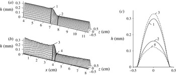
Shape of low-frequency wave for WGS rivulet compared with experimental data (Alekseenko et al.
Reference Alekseenko, Bobylev, Guzanov, Markovich and Kharlamov2010) at
 $\mathit{Re}_{m}=10$
,
 $f=1~\text{Hz}$
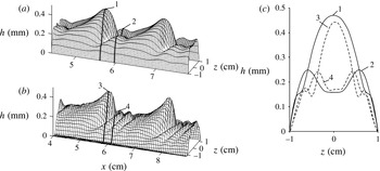
: (a) calculated 3D surface; (b) experimental 3D surface; (c) rivulet cross-sections; (1, 2) calculation; (3, 4) experiment.

Shape of developed wave for WGS rivulet compared with experimental data (Alekseenko et al.
Reference Alekseenko, Bobylev, Guzanov, Markovich and Kharlamov2010) at
 $\mathit{Re}_{m}=36$
,
 $f=23~\text{Hz}$
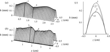
: (a) calculated 3D surface; (b) experimental 3D surface; (c) rivulet cross-sections; (1, 2) calculation; (3, 4) experiment.

Shape of developed wave for WGS rivulet compared with experimental data (Alekseenko et al.
Reference Alekseenko, Bobylev, Guzanov, Markovich and Kharlamov2010) at
 $\mathit{Re}_{m}=10$
,
 $f=15~\text{Hz}$
: (a) calculated 3D surface; (b) experimental 3D surface; (c) rivulet cross-sections; (1, 2) calculation; (3, 4) experiment.

Shape of developed wave for WES rivulet compared with experimental data (Alekseenko et al.
Reference Alekseenko, Bobylev, Guzanov, Markovich and Kharlamov2010) at
 $\mathit{Re}_{m}=25$
,
 $f=17~\text{Hz}$
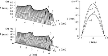
: (a) calculated 3D surface; (b) experimental 3D surface; (c) rivulet cross-sections; (1, 2) calculation; (3, 4) experiment.

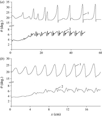
Dependencies of contact wetting angle on distance for nonlinear waves with frequency of (a) 5 Hz and (b) 15 Hz at
 $\mathit{Re}_{m}=25$
. Curve 1 is for a WES rivulet and curve 2 is for a WGS rivulet.

A numerical simulation of rivulet wave motion is performed for the experimental conditions according to Alekseenko et al. (Reference Alekseenko, Bobylev, Guzanov, Markovich and Kharlamov2010). Therefore, let us further consider the calculated results, which correspond to the experimental data. Figure 11 shows the low-frequency developing wave in comparison with the experimental data for the WGS rivulet at
 $\mathit{Re}_{m}=10$
,
 $f=1~\text{Hz}$
and
 $b=4\times 10^{-3}~\text{m}$
. At such a low frequency, a solitary step-wise wave is formed near the inlet. The comparison shows that the calculation accurately describes the wave surface and rivulet profiles in the vicinity of the step. The existence of waves with a step-wise shape is a distinctive feature of the rivulet flow because, in the case of the film flow, the excited step-wise waves are rapidly destroyed, thus forming a sequence of solitary-type peaks, as shown by Alekseenko et al. (Reference Alekseenko, Nakoryakov and Pokusaev1985). Figure 12 illustrates the shape of the developed waves on a WGS rivulet and compares them with experimental data for sufficiently high Reynolds numbers and forcing frequencies (
 $\mathit{Re}_{m}=36$
,
 $f=23~\text{Hz}$
,
 $b=1\times 10^{-2}~\text{m}$
). The figure clearly shows that the calculation accurately describes the shape of the peak with capillary ripples in front of a wave peak as well as rivulet profiles for different cross-sections. A significant discrepancy with the experimental data is observed in terms of the wavelength. The predicted distance between peaks is
 $1.5\times 10^{-2}~\text{m}$
, whereas the experiment yields
 $2\times 10^{-2}~\text{m}$
. In figure 13, the comparison of the calculation with the experimental data is performed for the case of the WGS rivulet at
 $\mathit{Re}_{m}=10$
,
 $f=15~\text{Hz}$
and
 $b=4\times 10^{-3}~\text{m}$
when the wave profile is sufficiently smooth and without intermediate small-scale ripples. The figure demonstrates that the calculated shape of the wave and the rivulet cross-sections of the wave crest and trough are in fair agreement with the experimental data. However, a certain mismatch remains in terms of the wavelength; the calculated value is
 $1.25\times 10^{-2}~\text{m}$
, whereas the experimental value is
 $2\times 10^{-2}~\text{m}$
. Figure 14 shows the developed wave in the WES rivulet at
 $\mathit{Re}_{m}=25$
,
 $f=17~\text{Hz}$
and
 $b=1.7\times 10^{-3}~\text{m}$
and compares it with experimental data. Figure 14 clearly shows that the model predicts the shape of the rivulet wave surface, except for one feature: no narrow additional crest in front of the main peak is predicted by the calculations. There is also a discrepancy in terms of the wavelength: the calculated value is
 $2.2\times 10^{-2}~\text{m}$
, whereas the experimental value is
 $3.1\times 10^{-2}~\text{m}$
. In the calculations of the wave for WES rivulet, no capillary ripple ahead of the main peak is found in the entire studied frequency range, which is consistent with the data of Alekseenko et al. (Reference Alekseenko, Bobylev, Guzanov, Markovich and Kharlamov2010). The divergence between the calculation and experiment in terms of the wavelength (at the same forcing frequency) is observed in the investigated frequency range. This divergence is caused by the difference in the calculated and experimental values of the wave propagation velocity. The difference in wave velocity, which was also discussed in § 3.2, is possibly related to the assumption of a self-similar velocity distribution, which is accepted for many problems of film flow but is insufficiently validated for a rivulet wave flow at
 $\mathit{Re}_{m}\sim 10$
due to the lack of experimental data.
Although Alekseenko et al. (Reference Alekseenko, Bobylev, Guzanov, Markovich and Kharlamov2010) found a weak sensitivity of the contact angle to the wave phase in the rivulet, such a conclusion is not reliable. The profile of the wavy rivulet cross-section obtained from processing experimental data near the contact line is severely distorted; therefore, there is arbitrariness in the determination of the contact angle in a disturbed rivulet. Figure 15 shows the calculated values of the contact wetting angle as a function of the distance for nonlinear waves on the surface of the WES and WGS rivulets at frequencies of 5 and 15 Hz. All calculations were performed assuming a constant width of the rivulet (fixed contact line). In both cases, the contact wetting angle exhibits large oscillations in accordance with the wave phase. Moreover, the amplitude of the contact angle oscillations increases with increasing wave amplitude. For the WGS, the amplitude of the contact wetting angle oscillations is significantly smaller than that for the WES. For the WES rivulet, the pulsation amplitude at a frequency of 5 Hz is considerably higher than that at 15 Hz, and for the WGS rivulet, the pulsation amplitudes at both frequencies are approximately equal.
4. Conclusion
A numerical simulation of linear and nonlinear three-dimensional forced waves in a rectilinear rivulet flowing down a vertical plate has been performed. The calculations were carried out for two liquids (WES and WGS) with different physical properties that were used in experiments of Alekseenko et al. (Reference Alekseenko, Bobylev, Guzanov, Markovich and Kharlamov2010). The dispersion curves for linear waves are calculated in the form of dependencies of the velocity propagation
 $C$
and spatial increment on the frequency
 $f$
. Compared with the film flow, the waves in rivulets exhibit significant differences. These differences result from the fact that the rivulet flow is characterised by an additional parameter
 $h_{0}/b$
, which influences the wave characteristics. In particular, the wave patterns for the cases of ‘small’ and ‘large’ contact wetting angles are significantly different. The calculations show that for the WES rivulet (‘large’ contact wetting angle), the waves are two-dimensional in nature, whereas for the WGS rivulet (‘small’ contact wetting angle), three-dimensional horseshoe-shaped waves develop. This is related to both linear and nonlinear waves in the investigated frequency range. A comparison of experimental data on nonlinear waves with the calculations, which were performed for different Reynolds number within a wide range of forcing frequencies, leads to the following conclusions. The applied model is appropriate for describing the shape and amplitude of the waves on the rivulet surface at moderate Reynolds numbers. In particular, for the WGS rivulet, the model predicts step-wise waves, which were observed in the experiments at low forcing frequencies. For moderate forcing frequencies, the model predicts waves with capillary ripples in front of the wave peak. The shape of these waves is in good agreement with the experimental data. For the WES rivulet, the model accurately predicts the amplitude of the developed waves and the shape of the rivulet wave surface, except for one feature: no narrow additional crest in front of the main peak is predicted by the calculations. In addition, for the WES rivulet, the model predicts no capillary ripple in front of the main peak, which is consistent with the data of Alekseenko et al. (Reference Alekseenko, Bobylev, Guzanov, Markovich and Kharlamov2010). The calculations have shown that for a wave rivulet flow, the value of the contact wetting angle oscillates noticeably in accordance with the wave amplitude and phase (under the condition
 $b=\text{const.}$
). The velocity of nonlinear stationary waves in rivulets is linearly related to their amplitude, which is similar to the cases of two-dimensional waves in liquid films and three-dimensional waves on rivulets flowing along the lower surface of an inclined cylinder.
There is a significant difference between the results of the numerical simulation and the experimental data in terms of the wave velocity (and, thus, the wavelength). The calculated values of the wave velocity are
 $1.4$
–
 $1.6$
times smaller than the experimental values. A possible reason for this discrepancy may be the self-similar (parabolic) velocity profile used in the model by Demekhin & Shkadov (Reference Demekhin and Shkadov1984). The parabolic velocity profile is common in many problems of film flows but is insufficiently validated for three-dimensional wave motion in rivulets, especially for the transverse component of the velocity. There is an apparent need for more detailed experimental studies on the wave motion of rivulets in a wider range of flow parameters.
The principal feature of the considered problem is that for a rectilinear rivulet on a vertical wall, three-dimensional, nonlinear, steady-state travelling waves can be realized in a wide range of options, which is practically impossible to observe in film flows. Thus, a detailed study of determinate, three-dimensional, nonlinear wave processes can be performed, which is a rarity for hydrodynamic systems.
Acknowledgements
This work was supported by the Russian Science Foundation (project no. 14-29-00093 for numerical simulations and project no. 14-22-00174 for experimental study).