1. Introduction: The Received Theory of Causal Nets
One of the best developed contemporary accounts of causality is the theory of causal nets (TCN). While most earlier accounts attempted to explicate causality by means of definitions, the TCN account characterizes causality via axiomatic principles that explain probabilistic relations of (in)dependence between variables by the existence of directed causal relations between them. This realistic understanding of TCN is informally acknowledged by Spirtes, Glymour, and Scheines (Reference Spirtes, Glymour and Scheines1993, secs. 3.4–5) and Pearl (Reference Pearl2009, preface, viii–ix), although both Pearl and Spirtes et al. present TCN’s axioms as definitions (Spirtes et al. speak of “axioms” on pp. 4 and 29). An explicitly axiomatic reconstruction of TCN is given in Schurz and Gebharter (Reference Schurz and Gebharter2016).
This section gives a brief exposition of the notions and axioms of TCN. A (mathematical) variable is a measurable function X:  from a domain D of individuals to its value space
 , which is a family of properties or a set of numbers. If X denotes color, for example, then
 , and X assigns a color X(α) to every individual
 . The domain may also consist of n-tuples of individuals, for example, individuals at certain time points. Binary properties are represented by binary variables XF with value space {F,¬F}. Terminological conventions:
• X,Y,Z (possibly indexed) are variables, and U,V,W are sets of variables;
• lowercase x’s (or xi) stand for values of X, and lowercase u’s (or ui), for sets of values of the respective variables in U.
A causal graph is a pair (V,E), where  is a set of variables (the “vertices”) and
 a set of directed arrows
 (the “edges”).Footnote 1 A graph (V,E) together with a probability distribution P is called a causal model (CM) (V,E,P). When we use causal graphs or models to represent reality, we speak of causal structures or systems, respectively.
The symbol P denotes an objective probability distribution over a suitable algebra AL over the value space over V; that is, P:  (with corresponding projections to subspaces). Further terminological conventions:
• P(x) (or P({x})) abbreviates
 , that is, the probability that X takes value x in the underlying domain D (the individual variable α is bound by P).
• Likewise, P(S) stands for
, P(¬x) for , P(x,y) for , and for , that is, the conditional probability of x given y, provided .


Two variables X,Y are probabilistically dependent (DEP(X,Y)) if and only if (iff) some of their values are dependent; otherwise X, Y are probabilistically independent. More generally, probabilistic (in)dependence between X and Y conditional on (fixed values of) a set of variables U is defined as follows:
•
: and , and•
iff not , that is, iff ∀x,y,u: or .


If the variables’ values are ordered according to size, the notion of positive/negative dependence between variables can be defined as follows: X depends positively/negatively on  >/<
 (for all x1, x2, y1, y2).
A causal graph (V,E) is described by using the following notions:
 : X is a direct cause of Y (Y is a direct effect of X).
 : X is a causal ancestor of Y (Y is a causal successor of X); that is, there is a directed path
 from X to Y (for
 ).Footnote 2
 :
 or
 ; that is, X and Y are adjacent.
 : a path
 between X1 and Xn that connects X1 and Xn; the variables Xi (
 ) are said to lie on this path.
If Xi lies on a path π, then Xi is called (i) a common cause, (ii) an intermediate cause, or (iii) a common effect on π iff (i) ←X→, (ii) ←X← or →X→, or (iii) →X←, respectively, is part of π.
The set of all direct causes of a variable X is called the set of its parents, Par(X). Note that TCN is compatible with ontological indeterminism; that is, the values of Par(X) need not determine the value of X. Determinism in regard to variable X is given when for all possible values  there exists an
 with
 .
TCN explains probabilistic dependencies via causal connections by means of two core axioms: causal d-connection (C) and minimality (Min). Variable C is frequently expressed by the equivalent causal Markov condition (M) (Spirtes, Glymour, and Scheines Reference Spirtes, Glymour and Scheines2000, sec. 3.4.1). We prefer C over M for reasons specified below. The axiom C states that every (conditional) probabilistic dependence between two variables X and Y is the result of a causal “d-connection” between X and Y:
(1) Definition: A CM (V,E,P) satisfies the condition C of causal d-connection iff for all X,  and
 : if
 , then X and Y are d-connected given U in the following sense: X and Y are connected by some path π such that
(SIC): no intermediate cause on π is in U,
(SCC): no common cause on π is in U, and
(CE): every common effect on π is in U or has a causal successor in U.
Axiom: Every physically possible causal system that is [sufficiently] complete satisfies condition C.
In (1) we distinguish between the definition of the causal d-connection condition and the corresponding axiom, which states that this condition holds for all physically possible systems that are either complete or at least sufficiently complete (as indicated by the square brackets); these two notions of completeness are characterized below.
Two variables X, Y are “d-separated” given U if they are not d-connected given U. The concepts of d-separation and d-connection were developed by Pearl (Reference Pearl1988, 117). Axiom C asserts an implication from (probabilistic) dependence to d-connection, or in contraposed form, from d-separation to independence (Pearl Reference Pearl1988, 119; Reference Pearl2000, theorem 1.2.4). Axiom C implies the standard causal principle for unconditional dependence: if DEP(X,Y), then X and Y are connected by a directed or common cause path (i.e., d-connected by the empty set ∅).
Our formulation in (1) makes it plain that condition C entails three independent principles:
SIC (screening off by intermediate causes): Direct causes screen off indirect causes from their effects. Thus, in a [sufficiently] complete CM of the form  ,
 holds. Condition SIC goes back to Andrei Markov (senior).
SCC (screening off by common causes): Common causes screen off their effects from each other. So in a [sufficiently] complete CM of the form  ,
 holds. Condition SCC goes back to Reichenbach (Reference Reichenbach1956).
CE (common effects): The causes of a common effect are unconditionally independent but may be dependent conditional on a common causal successor. Thus, in a [sufficiently] complete CM of the form  ,
 holds, and
 will hold if the CM is faithful (see definition (3)). Condition CE was discovered by Berkson (Reference Berkson1946) and is called Berkson’s paradox.
The full content of these three principles is expressed as follows: “If  , then there is an X-Y-connecting path π such that (P),” where P is one of the clauses SIC, SCC, or CE in (1), respectively.Footnote 3 The modularization of axiom C into three entailed principles is important for our purpose of revision because it allows us to alter one part of C without changing the others.
A causal graph (model) is acyclic iff it contains no cyclic path  . In this article we concentrate on acyclic graphs. For acyclic CMs, condition C is equivalent to the causal Markov condition M (Spirtes et al. Reference Spirtes, Glymour and Scheines2000, theorem 3.3; Pearl Reference Pearl2009, 16):
(2) Definition: (V,E,P) satisfies the causal Markov condition M iff every  is independent of any subset
 of nonsuccessors of X, conditional on X’s parents:
 .Footnote 4
The equivalence between M and C has been demonstrated by Verma and Pearl (see Pearl Reference Pearl1988, 119–20, theorem 9) and Lauritzen et al. (Reference Lauritzen, Dawid, Larsen and Leimer1990). The latter authors call C the global and M the local Markov condition, since in its contraposed form, C asserts a (conditional) independence for all d-separation relations of a causal graph, while M asserts such an independence only for the d-separation relations between a variable X and its noneffects conditional on its parents; the other independencies follow from these as probabilistic consequences. For this reason, C expresses the full content of the causal Markov condition in a more transparent way than M. Moreover, the three principles SIC, SCC, and CE are more directly contained in axiom C than in condition M.
The explicit distinction between the definition of C and the axiom C in (1) impels us to critically reflect on the problem of generality: do all probabilistic dependencies between analytically independent variables in fact result from causal d-connections? This has been a question of debate for several decades. Two remarks on this debate are important for our purpose: First, although the criticism was often directed against the Markov condition “in general,” our reconstruction of axiom C as entailing three independent conditions helps us to locate the problem: what was under attack was not condition SIC or CE but only SCC—screening off by common causes. Second, defenders of TCN usually acknowledge that SCC fails in application to far-distance (EPR/Bell) correlations in quantum mechanics, but they regard SCC as valid for all other domains (Spirtes et al. Reference Spirtes, Glymour and Scheines2000, 37–38; Pearl Reference Pearl2009, 62). Only a few authors, foremost Cartwright (e.g., Cartwright Reference Cartwright2007), have insisted that the causal Markov condition may fail for macrophysical systems as well. Section 2 will support this position, but since the counterexamples only concern subcondition SCC of C, we argue in section 3 that the Markov condition should not be abandoned but should be revised in certain ways.
Axiom C asserts an implication from probabilistic dependence to d-connection. The converse implication from d-connection to probabilistic dependence is called the condition of faithfulness (Spirtes et al. Reference Spirtes, Glymour and Scheines2000, 31; Zhang and Spirtes Reference Zhang and Spirtes2008, 24):
(3) Definition: A CM (V,E,P) satisfies the faithfulness condition F iff for all X,  and
 : if X and Y are d-connected given U, then
 .
To avoid confusion, note that Spirtes et al. (Reference Spirtes, Glymour and Scheines2000, 31) define “faithfulness” as the conjunction of conditions C and F. We prefer definition (3) (which is also used in Zhang and Spirtes Reference Zhang and Spirtes2008, 247) because it logically separates F from C. This is essential for our revision, which does not concern F but only one part of C (i.e., SCC).
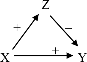
The probability distributions over the variables Xi of a CM conditional on their parents,  , are called the parameters of the CM (Pearl Reference Pearl2009, 44). It is well known that the faithfulness condition may fail for CMs whose parameters are fine-tuned in a such way that the influences of two (or more) d-connecting paths are opposite and cancel each other out. An example is presented in figure 1.
Unfaithful causal graph:  but INDEP(X,Y), because the positive influence
 and the negative influence
 cancel to 0. Here
 means that the arrow
 is responsible for a positive/negative dependence of Y on X (as explained), conditional on
 . See Schurz and Gebharter (Reference Schurz and Gebharter2016), (9), theorem 2.

Therefore, condition F is not suited as a general axiom of TCN. Proponents of TCN argue that the satisfaction of F is at least highly probable because unfaithful CMs are parameter instable, in the sense that their unfaithful independencies can be destroyed by arbitrary small changes of the parameters of the CM (Pearl Reference Pearl2009, def. 2.4.1). This fact implies that unfaithful independencies are statistically rare in all causal systems that are subject to external noise variables that are mutually independent and, thus, produce independent variations of the system’s parameters.
However, there is a weakening of F that holds in full generality and constitutes TCN’s second core axiom—the condition of minimality (Spirtes et al. Reference Spirtes, Glymour and Scheines2000, sec. 3.4.2):
(4) Definition: A C-satisfying CM (V,E,P) satisfies the minimality condition (Min) iff no arrow can be omitted from E without violating condition C.
Axiom: Every physically possible C-satisfying causal system satisfies Min.
In contrast to axiom C, axiom Min can be justified by a methodological requirement that is a variant of Ockham’s razor: causal arrows are only assumed if they are responsible for at least some (conditional) probabilistic dependence, for values that either are factually realized or can be brought about by interventions.Footnote 5
Schurz and Gebharter (Reference Schurz and Gebharter2016, sec. 3) investigate whether the theory TCN has empirical content by which it can be independently tested. Since causal arrows are regarded as theoretical (unobservable) relations, the TCN would have empirical content if it excluded logically possible probability distributions, that is, if there were probability models (V,P) that cannot be extended to TCN-satisfying CMs. The authors prove that the core of TCN, axiomatized by C + Min, is without empirical content. If an axiom of cautious faithfulness is added to C + Min—“cautious” in the sense that it asserts faithfulness merely with high probability—this extended version of TCN acquires weak probabilistic content. More empirical content is obtained if one adds to TCN the axiom of temporal forward-directedness T. This axiom applies to CMs whose variables are event variables, that is, variables Xi whose values are possible events having a location in time, t(Xi). For these CMs condition T states that (for all X,  )
 implies
 ; that is, causes precede their effects in time. The extension of C + F by T excludes a variety of logically possible probability distributions (Reference Schurz and Gebharter2016, sec. 3.3).
Several objections against the truth of the causal Markov condition have been successfully defeated by proponents of TCN (see Spirtes et al. Reference Spirtes, Glymour and Scheines2000, 59–63; Pearl Reference Pearl2009, 62; Hitchcock Reference Hitchcock and Zalta2010). In particular, it has been shown that C can only be true if
a) the variables in V are analytically independent; otherwise one obtains “arrows” on purely conceptual grounds (Hitchcock Reference Hitchcock and Zalta2010, secs. 2.3, 2.10), and
b) the description of the causal system is sufficiently refined (cf. Haussman and Woodward Reference Haussman and Woodward1999, 527–29).
Since the omission of certain variables or edges from a C-satisfying CM can lead to a violation of C, axiom C refers prima facie to physically possible CMs that are complete in the following sense:
(5) Definition: (V,E,P) is a complete physically possible CM iff (V,E,P) is true in a physically possible world w and every variable in w that is a direct cause or effect of a variable in V is itself in V and its attached edges are in E.
Unfortunately, complete causal systems are typically not epistemically accessible. What does condition C entail for coarse-grained descriptions of causal systems that omit some detail and, thus, are incomplete?
A structural coarsening of a CM removes some variables and their edges but preserves cause-effect relations between the remaining variables. It is well known that the satisfaction of condition C is not preserved by every structural coarsening of a CM but only by structural coarsenings that are causally sufficient, that is, do not remove a common cause (Spirtes et al. Reference Spirtes, Glymour and Scheines2000, 22, 27). However, there is a second kind of coarsening that plays a role in the next section and is called conceptual coarsening. Here a CM is described with the help of a compound variable Z that is definable in terms of more fine-grained variables X1, …, Xn; we write  . When a model is conceptually coarsened by a compound variable Z, then the set of defining variables X1, …, Xn is replaced in V by the compound variable Z and an arrow between a variable Y and Z is added whenever the original model contained a corresponding arrow between Y and some defining variable of Z. This operation is illustrated in figure 2.
Coarsening of causal graph G1 by the compound variable Z = f(X1, X2, X3).

Assume that in the refined model M1 of figure 2 axiom C is violated because  holds (since X2 is an interactive cause; see sec. 2). Nevertheless
 holds in M1; thus, by assuming f to be injective,
 will hold in M2 (since each value triple [x1,x2,x3] is uniquely translated into one Z-value z = f[x1,x2,x3]). So M2 satisfies C, although its conceptual refinement M1 fails to satisfy C. This shows that a conceptual coarsening of a CM may hide a violation of C.
To sum up, the satisfaction of C by a complete CM M* does not imply that a coarsening of it will satisfy C, nor does the violation of C by M* imply that a coarsening of M* will violate C. What can be guaranteed is that a CM is “sufficiently complete,” in the sense of not distorting the true laws of causality, if its variables describe reality at the most fine-grained level and do not omit true common causes. Turning this into a definition would not be very useful, however, since most descriptions of reality are coarse-grained. All that can be said of coarse-grained descriptions is this:
(6) If C is satisfied by every complete causal system of a world w, then every coarse-grained CM that is true in w has a true refinement in w that satisfies C.
Although condition 6 is analytically true, it gives us a heuristic for testing C:
(7) Test heuristic for C: If a true causal model M is found such that not only M but every true refinement of M that is consistent with the established background knowledge violates C, then the truth of C in the actual world is strongly disconfirmed. On the other hand, if all CMs considered so far satisfy C for all plausible refinements of them, then C is confirmed.
In the next section we will make use of this heuristic.
2. Interactive Causes: Violation of SCC in Indeterministic Decay Processes
Given that axiom C is empirically empty in isolation, how can the truth of C be tested by empirical means at all? Following from the results concerning the empirical content of TCN mentioned in section 1, there are two ways of testing axiom C: either one strengthens C by condition F or by condition T. It is natural to assume condition T in the counterexample to which we now turn, namely, the example of spontaneous decay. However, our arguments do not presuppose this condition: we will see that even without assuming T certain causal structures involving spontaneous decay violate axiom C with high plausibility, because they cannot satisfy C in a faithful way.
The example of spontaneous decay has been given in the literature several times, but it was often presented as if it were a specific aspect of quantum mechanics (cf. van Fraassen Reference Van Fraassen1980, 29–30; Arntzenius Reference Arntzenius and Zalta2010, sec. 2.1). In contrast, Cartwright (Reference Cartwright2007, 122) has emphasized that the counterexample only requires an indeterministic decay process. Indeterministic processes are found not only in quantum physics but also in classical physics.Footnote 6
Consider a particle (of type) q that decays with a certain probability p into two particles (of types) q1 and q2. The decay is objectively indetermined; that is, the probability of q’s decay conditional on all common causes in the past is (significantly) smaller than 1; however, if the particle decays, then it always (or almost always) decays into q1 and q2. Or at least: If q decays and one decay product is q1, then the other decay product is (almost) always q2. Examples are radioactive decay (e.g., the α-decay of uranium  ), spontaneous chemical decay (e.g., the decay of ethene
 ), or in everyday life the spontaneous breaking of an eroded mountain rock into two pieces, and so on.
What leads to a violation of SCC is the combination of two factors, (i) indeterminism plus (ii) the law describing a decay. Physically speaking the latter is an instance of a conservation law. Generally speaking, a conservation law for a quantity X says that the sum of the X-values of all parts of a closed system remains constant through time. Classical macrophysical or chemical decay is described by the conservation of mass (m): if q decays into q1 and q2, then  . This explains qualitative decay laws as follows: if q decays into two parts and one part is q1, then the other one must be q2, because q2 is the only physically possible decay component for that type of decay that conserves mass, via
 . More general conservation laws of physics, such as the conservation of energy, momentum, and charge, give rise to a more general notion of indeterministic decay that is introduced at the end of this section. In the next couple of paragraphs we discuss simple qualitative decay.
To reconstruct qualitative decay processes, we assume binary variables Qi that apply to spatiotemporal locations α of a small but finite size as their domain. The value of Qi(α) indicates whether a given type of particle qi is present ( ) or absent (
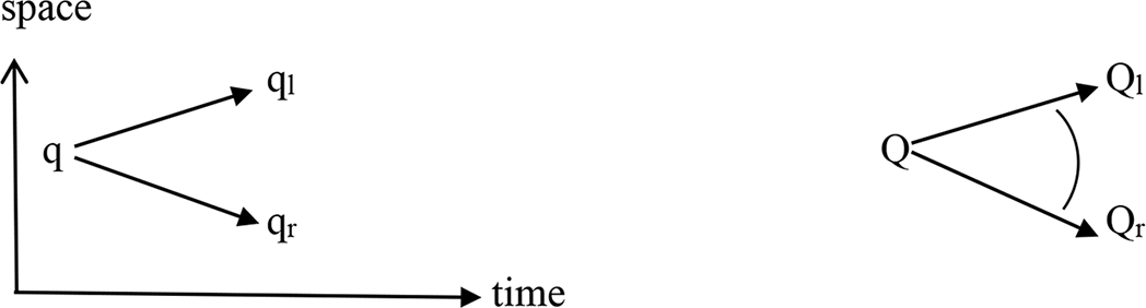
 ) at the location α or in a certain neighborhood f(α) of α that is determined by a spatiotemporal function f; in the latter case the variable carries “f” as a second index: Qf,i. In what follows, we consider a symmetric decay process in which a particle q decays into two type-identical particles ql and qr that are moving away from each other in opposite directions (see fig. 3). We let Ql(α) be the binary variable denoting the (non)occurrence of a particle ql shortly after the decay time at the left spatial side of α and Qr(α) the (non)occurrence of qr at the right side of α.
Indeterministic decay: Spatiotemporal diagram (left) and causal graph (right). Particle q (described by variable Q) decays into decay products ql and qr (described by Ql and Qr, respectively). SCC fails since neither Q nor any extended set of common causes in the past screens off Ql from Qr. “Q” is called an interactive (common) cause and is graphically represented by the arc.

Since neither the state of the particle Q nor any further variable before the decay screens off Ql from Qr, condition SCC of C is violated:  ; that is,
 . Moreover,
 holds for any set “Past” of variables describing events before the decay time.
Note that for the violation of SCC one need not assume that the conservation law holds with probability 1; it suffices that it holds with a probability p′ higher than the decay probability p. We follow Salmon (Reference Salmon1984, 158–77) and call a common cause that does not screen off its effects an interactive (common) cause and a common cause that does screen off its effects a conjunctive cause.
There are four prominent defense strategies for SCC against this type of counterexample:
(I) Value refinement of the interactive cause: Salmon’s example of an interactive cause was one of deterministic physics. Spirtes et al. (Reference Spirtes, Glymour and Scheines1993, 63) argued that if in that example the state of particle q immediately before the decay were described with maximal precision, it would imply the values of Ql and Qr with probability 1 and, thus, screen them off. However, in our example particle q decays only with a certain probability, so this defense does not apply.
(II) Linking the effects: One way to reconcile interactive forks with condition SCC is to add a direct causal link between the two effects (see fig. 4a). This possibility is typically excluded in the given examples of indeterministic decay because the two effects occur simultaneously; so a causal link between them would violate condition T, which holds in classical and relativistic physics because of their assumption of locality. In contrast, in quantum mechanics it is debated whether nonlocal causal links should be admitted (see Wood and Spekkens Reference Wood and Spekkens2015, 14ff.; Näger Reference Näger2016).
Defense strategies against the counterexample in figure 3. a, Linking the effects; b, hidden common cause; c, hidden intermediate cause.

Even without the assumption of condition T, the causal reconstruction in figure 4a leads to the problem of unexplained violations of faithfulness. There is a crucial difference between the conditional dependence between effects of an interactive cause and that between effects of a common cause with an additional causal link between them. In a faithful reconstruction of the latter model this causal link can be used to transmit the influence of an intervention on one effect to the other effect conditional on the common cause, but this is impossible in the case of an interactive fork. In our example of decay, such an intervention could be realized by positioning a device at the left side of α that emits particles of type ql so that the probability of finding p1 conditional on the presence of q is increased, compared to the distribution without this device. Formally,  , where P is the preintervention and PI the postintervention distribution. While in the case of indeterministic decay, the postintervention probability of the other decay product qr would be unchanged (
 ), it would be increased in a faithful version of figure 4a (
 ). In what follows we call this characteristic feature of interactive forks the nontransmission condition. In section 3 we demonstrate that a C-satisfying reconstruction of this feature is not possible without postulating mysterious unfaithful independencies.
(III) Introduction of a hidden common cause: Pearl (Reference Pearl2000, 62, fig. 2.6) suggested explaining  by assuming an additional hidden common cause Q* that together with Q screens off Ql from Qr (
 ; see fig. 4b). However, this defense strategy cannot explain a second characteristic feature: Interactive cause variables screen off their common effects when their value is “off,” that is, when the decaying particle or conserved quantity is absent. To see this, assume that even if there is no particle q in the spatiotemporal region α there is a small probability that a subparticle
 spontaneously appears in the left/right neighborhood of α, because it has moved in from the environment. Since the spontaneous appearances of ql and qr are mutually independent,
 must hold. However, this feature is not explained by the graph in figure 4b: Since the two common causes Q and Q* are causally unconnected,
 cannot entirely screen off Ql from Qr because of the influence of Q*. The common cause scenario could only explain this feature if a directed arrow led from Q to Q* that inactivates Q* whenever Q is absent,
 . But then Q* would play the role of an intermediate cause, which is the fourth defense strategy to be discussed below. We call this second characteristic feature of interactive causes the absence condition. It becomes important in a revised search procedure for interactive CMs.
(IV) Introduction of a hidden intermediate cause: Even if the particle decays with a probability of less than 1, many authors have argued for the existence of some intermediate cause q* (described by variable Q*) in the form of a breaking event or state of the particle immediately before the decay, so that q* causes the decay with certainty and, hence, Q* screens off Ql from Qr (see fig. 4c). This defense strategy is, for example, used by Haussman and Woodward (Reference Haussman and Woodward1999, 563) against Cartwright’s counterexample (Reference Cartwright2007, 122), in which a chemical process C succeeds 80% of the time, and when it succeeds it invariably produces two end products, a chemical X and a pollutant Y. These authors assume a certain intermediate event, the “operation of firing F,” that deterministically produces X and Y and screens off X from Y.
In this defense strategy the idea is to try to find a description of the decay process that makes it deterministic. The refutation of this strategy is more involved. We will present three arguments to show that this strategy either violates the assumption of indeterminism or rests on the artificial effects of a too coarse-grained description.
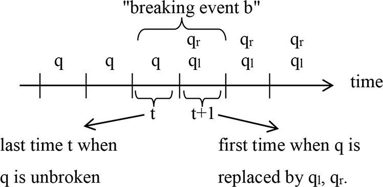
Argument 1: The first argument says that a breaking event is nothing but a temporal succession of two consecutive events or states: at time t, the particle q is still in the unbroken state, while at the next time point, it is in the “broken state,” which means that instead of q we now have the two decay products ql and qr, possibly very close together but already separated. If we reconstruct this in a discrete time, the picture is as in figure 5.
Reconstruction of a “breaking event” in discrete time.

Since the breaking event  is a compound of both the cause and its direct effects, it screens off its direct effects trivially; that is,
 holds for analytical reasons; the screening off of the indirect effects follows from this by condition SIC. As soon as we refine the description and discriminate between the events at time t and at time
 , the screening off disappears.
Proponents of this defense strategy tend to reply to this argument with the objection that time is continuous, so there are no such two consecutive time points t and  . A closer analysis shows that the continuity assumption cannot rectify the violation of the causal Markov condition. If time is continuous, two cases are possible: in case 1, there is a last time point
 at which q is unbroken, while for all times
 the particle is broken. Thus, the set of times for which the particle is unbroken forms a right-closed interval and the set of times for which it is broken an adjacent left-open interval (see fig. 6a). Then for all times
 Q(t) does not screen off Ql(t′) from Qr(t′), which is a violation of condition SCC.
Two possible reconstructions of a “breaking event” in continuous time. a, t = last time at which q is unbroken; unbroken state: right-closed interval “]”; broken state: left-open interval “(.” b, t = first time at which q is broken; unbroken state: right-open interval “)”; broken state: left-closed interval “[.”

Alternatively, in case 2 there is a first time point  at which q is replaced by its decay products ql and qr. Then the set of times for which the particle is unbroken forms a right-open interval, and the set of times for which it is broken, an adjacent left-closed interval (see fig. 6b). Then for all times
 Q(t′) does not screen off Ql(t) from Qr(t), which is again a violation of SCC.
Argument 2: The first argument shows that for every analysis of a breaking event as a succession of fine-grained events condition SCC fails. Some proponents of SCC reply to this argument as follows: although this may be so, it is at least possible to describe the causal structure in such a way that SCC holds, namely, by using the compound variable of a “breaking event.” At this point our test heuristic of section 1, condition 7, comes into play. What the defender of SCC says with this objection is, in effect, that SCC holds merely because the description is coarse-grained and hides the failure of SCC, which appears in all refined models that decompose the breaking event into a succession of fine-grained events. By test condition 7 this is strong reason to suppose that condition SCC is violated in the actual world.
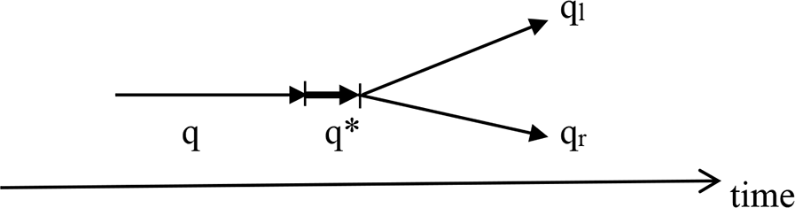
Argument 3: The objection remains that the “breaking event” is more than an instantaneous event consisting of a mere succession of an unbroken and a broken state. Rather, it refers to a specific prebreaking stage q* that the particle enters shortly before it decays (see fig. 7).
Particle q enters a prebreaking state q* before it decays.

Even if this assumption is made, the analysis given in the previous argument applies: either there is a first time point t at which the particle is broken (i.e., q* is replaced by q1 and q2), or there is a last time point at which the particle is unbroken (i.e., q* exists). If the decay is indeterministic, then in both cases condition SCC is violated. The only way to save condition SCC is to assume (as in argument 1) that the transition from the prebreaking state q* to the decay products ql and qr is deterministic. But this is implausible, since according to contemporary scientific understanding, radioactive decay or the breaking of chemical bonds (etc.) are indeterministic processes. Moreover, why should we assume that although the beginning (the left end) of the particle’s prebreaking stage is an indeterministic process ( ), its ending (the right end) should be a deterministic process? This seems too strange to be plausible: if the decay process is indeterministic, then it is indeterministic “on both sides.” To summarize, in all plausible reconstructions of indeterministic decay processes, the particle’s state before the decay does not screen off the states of its decay products.
So far we have only analyzed simple (qualitative) indeterministic decay, in which the decay itself occurs spontaneously. However, the same reasoning applies in cases of generalized indeterministic decay: here the decay event may have a deterministic cause, but a conserved quantity X of the unbroken particle q is indeterministically distributed over its decay products, in the sense that (i)  is small but (ii)
 is (close to) 1. Conditions i and ii imply the interactive fork condition
 . As an example, consider the generalized decay of a high-energy gamma particle (γ) into a positron (e+) and an electron (e−), which is also called “pair creation.” It is caused by the clash of a γ particle against an atomic nucleus a. Since the momentum
 of the γ particle is absorbed by a (
 ), the total momentum of p and e must be 0 (
 ). This means that e+ and e− fly apart in opposite directions, but the particular direction (and momentum) is undetermined. This leads to the interactive fork conditions i and ii above, if we substitute γ for q, e+ for ql, e− for qr, and
 for X.
The notion of generalized indeterministic decay also applies to far-distance correlations in quantum-mechanical EPR/Bell experiments. Here a source emits a pair of entangled particles (e.g., electrons) flying in opposite directions. The interactive cause is the state of the entangled two-electron system q, whose total spin in the direction of the z-axis is conserved. Upon measurement at one of the two “sides” of the spatially extended two-electron system, q’s wave function collapses into a statistical ensemble of the states of the two separate electrons ql and qr. This collapse is described as a generalized decay. While conditional on the measurement this decay obtains with certainty, the total spin is indeterministically distributed over the two electrons, satisfying the conservation law  . Depending on the states (polarization angles) of the measurement devices Ml and Mr, measurement of S(ql) and S(qr) yields the results R1 and Rr, respectively (with
 ), whose distribution satisfies Bell’s famous inequality-violating correlations:
 (see Wood and Spekkens Reference Wood and Spekkens2015). In section 3 we argue that this correlation can be faithfully explained by an interactive cause but not by a common cause model. The difference from classical indeterministic decay does not concern the basic structure of an interactive fork but rather the nonlocal nature of the entangled system whose wave function stretches over a huge distance, although it is instantaneously influenced by measurements on either side of the electron pair.
The conclusion of this section is that in indeterministic decay processes (in the simple or generalized sense) condition SCC is violated. Philosophers who accept this conclusion may nevertheless defend the causal Markov condition by pointing out that indeterministic decays are exceptions that do not arise in everyday life or in the special (life or social) sciences. This does not seem to be true, either. An everyday life example of a violation of SCC is a rock q in the Alps from which a piece q1 breaks off spontaneously, leaving the now smaller rock q2 behind, with  . Given rock q at time t, the probability that in the next moment of time
 a piece q1 breaks off is low, but given q2 at time
 , with near certainty the missing piece q1 is in the (dangerous) state of falling downward at time
 .
Concerning the social sciences, we conjecture that quantities possessed by social groups (national wealth, etc.) may undergo processes of generalized decay: often the total amount of such a quantity remains fairly constant, while its social distribution undergoes unpredictable changes. An elaboration of this conjecture is left to the future.
In conclusion, it appears that violations of condition SCC due to interactive causes may occur in all domains. In the next section we develop a revision of condition C that accounts for interactive causes.
3. Revision of TCN
The minimal revision of TCN that accounts for interactive causes is to exempt interactive causes from the d-connection condition C, or more precisely, to exempt them from the set of nodes whose presence in the conditioning set blocks a d-connection. In what follows we call the minimal revisions of the notions of d-connection, condition C, and faithfulness “d*-connection,” “condition C*,” and “d*-faithfulness,” respectively. The unasterisked and asterisked notions coincide for CMs without interactive causes but differ in regard to interactive causes. We will argue that the minimal revision is the right revision, except for an additional constraint that accounts for the absence condition (recall sec. 2).
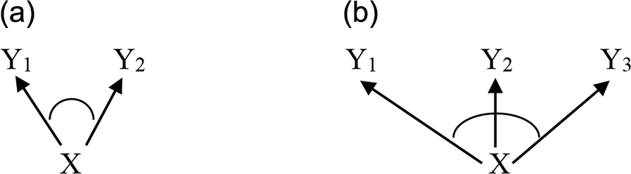
We display an interactive cause graphically by an arc that connects the arrows pointing toward its direct effects.Footnote 7 We call such an arc an interactive arc and assume that effects connected by such an arc are d*-connected conditional on their interactive cause (see fig. 8a); we also say they are “interactively d*-connected.” If the interactive CM is d*-faithful, then two interactively d*-connected effects will be probabilistically dependent conditional on their interactive cause; we say in this case that they are “interactively (probabilistically) dependent.” Moreover, an interactive cause may have more than two effects, as in figure 8b: an example is the β-decay of a neutron into proton, electron, and anti-neutrino.
Interactive forks are displayed by arcs connecting interacting arrows.

In section 2 we characterized the correlations between interactively d*-connected effects by the nontransmission condition, which distinguishes them from the conditional correlations between effects of a common cause that result from of a causal link between them. In the latter case, the conditional dependence between the effects can be used to propagate the influence of an intervention on the causing effect to the other effect (provided the CM is faithful). This is depicted in figure 9a, where Z1 figures as an intervention variable on the causing effect Y1: the result is  . In contrast, the conditional correlation between the effects of interactive causes cannot be used to propagate the influence of an intervention: in figure 9b
 holds.
Distinguishing correlations produced by directed arrows (a) from correlations produced by interactive causes (b). In both CMs (which are assumed to be faithful) we have  , but only in a do we have
 ; that is, Z1 can be used as intervention variable on Y1 with respect to Y2. In b
 holds (nontransmission condition).

Condition C* (the minimal revision of C) is sufficient to account for the behavior displayed in figure 9. It implies for figure 9a that Y2 is d*-connected (as well as d-connected) with Z1 given ∅ and given X, along the path  . For figure 9b it yields that Y2 is not d*-connected (or d-connected) with Z1 given ∅ or given X. To ensure d*-connection, the common effect Y1 has to be included in the conditioning set; that is, in figure 9b Y2 is d*-connected (and d-connected) with Z1 given Y1.
Condition C* has the further consequence that in figure 9b Y2 is d*-connected with Z1 given {X,Y1}, which is not the case for d-connection in figures 9b or 9a. Do we have a corresponding probabilistic dependence  in figure 9b? If the CM is d*-faithful, the answer is yes. Here is an intuitive example that illustrates this dependence: Assume that the interactive cause
 in figure 9b describes the spontaneous decay of particle q into q1 and qr, but the conservation law is not entirely deterministic (
 ), and Z1 is an additional factor whose presence increases the probability of ql’s presence (
 ) after the decay. Factor
 may represent a field that attracts ql particles and increases the probability that they fly into region α from outside it. Assume the particle decays (X = q) and the right decay product is absent (
 ). Then the absence of qr in spite of the presence of q increases the probability that the presence of ql was caused by
 . This means that
 ; that is,
 . Thus, the revised condition C* yields the correct result.
A noninteractive and d-faithful reconstruction of the (in)dependences characterizing figure 9b would be possible by inverting the direction of the causal arrow  in the CM of figure 9a; the resulting structure would explain
 ,
 , and
 . This is no longer possible, however, in the CM in figure 10a, which extends the CM in figure 9b by adding a second cause Z2 to Y2:
 . The (in)dependences characterizing this CM cannot be described by a noninteractive CM in a faithful way. To explain
 ,
 and
 in a d-faithful way, we would have to add the arrow
 to the CM without the arc above X. But this would turn
 into an d-unfaithful independence because then Z2 is d-connected with Y1 given X. Moreover, we would additionally need the arrow
 to explain
 . This unfaithful CM is depicted in figure 10b; the bold arrows generate unfaithfulness.
a, d*-faithful interactive CM whose (in)dependencies have no faithful noninteractive modeling; b, d-unfaithful CM of the (in)dependencies characterizing a (bold arrows generate unfaithfulness).

The example of figure 10a shows that there are d*-faithful interactive CMs that admit of no faithful noninteractive reconstruction. Thus, misidentifying an interactive as a conjunctive cause may lead to unfaithfulness. This fact may explain recent findings of Näger (Reference Näger2016) and Wood and Spekkens (Reference Wood and Spekkens2015, 2) who applied TCN to quantum-mechanical EPR/Bell correlations and conclude, in the words of Näger (Reference Näger2016, 12), that “the causal faithfulness condition and the causal Markov condition cannot both hold in the quantum realm.” Recall the EPR/Bell experiment described in section 2: if we identify the variable S(q) of this experiment (describing the spin state of the entangled electron pair q before measurement) with the variable X in figure 10a, the variables M1 and M2 describing the state of the measurement devices with Z1 and Z2 in figure 10a, and the variables R(ql) and R(qr) describing the measurement results with Y1 and Y2 in figure 10a, then we obtain the causal structure describing the EPR/Bell experiment. The nontransmission condition that characterizes interactive causes,  , corresponds to the famous “no signaling” condition. As we explained above, a C-satisfying reconstruction of the probabilistic (in)dependences in this experiment without assuming a hidden common cause is only possible if one introduces the additional arrows
 and
 that imply “superluminal causation” and generate unfaithfulness (Wood and Spekkens Reference Wood and Spekkens2015, fig. 23).Footnote 8 In contrast, the reconstruction of the EPR/Bell experiment as an interactive CM can explain all (in)dependencies of this experiment in a d*-faithful way. These remarks are intended as promissory notes concerning the applicability of the proposed account to quantum mechanics; working out the details would require a paper of its own.
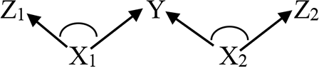
So far we have considered interactive effects having a further cause. In figure 11 we consider two interactive forks that are connected via a common effect. Here Z1 and Z2 are not d*-connected given {X1,X2} but are d*-connected given {X1,X2,Y}, that is, conditional on their common effect. By C* we get  , and by d*-faithfulness,
 . As an example, assume that two particles x1 and x2 decay into the partially overlapping decay products z1,y and y,z2, respectively. The presence of z2 conditional on x2 makes y’s presence more probable, but this probability increase is not propagated to z1 conditional on x1 because the decay of x1 is independent from that of x2. However, conditional on the presence of y, x1, and x2, the absence of z2 increases the probability that z1 is present because x1 decayed. Again the minimal revision gives the right result.
Two interactive causes may share an effect: Z1 and Z2 are d*-connected and dependent only if Y is in the conditioning set.

We finally turn to interactive causes with more than two effects, as in figure 8b above. We require that if more than two effects are connected by one arc, then each effect must be interactively dependent on at least one other effect. We consider this as the extension of the minimality axiom for d*-connections: Each d*-connection by an interactive arc must produce at least one interactive probabilistic dependence, so that removing this arc causes a violation of condition C*. But, interactive correlations within one arc need not always be transitive, so that all pairs of effects within one arc become interactively correlated; this is only the case if the interactive CM is d*-faithful.
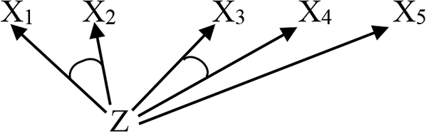
We admit the possibility that the same interactive cause produces two (or more) sets of interactive effects in separate interactive events. This is displayed in figure 12, in which {X1,X2} and {X3,X4} are sets of interactively d*-connected effects of Z; moreover, X5 is an additional conjunctive effect of Z. As an example, consider high-energy γ-rays (X) that create two different kinds of particle pairs, electron positrons (X1,X2) and muon antimuons (X3,X4), and in addition produce heat (X5). Following from the above requirement on arcs, different sets of interactive effects of one interactive cause are disjoint; that is, a variable in one set is merely conjunctively correlated with the variables in another set.
One interactive cause causes two interactive pairs of effects and one ordinary effect. Variables not connected by an interactive arc are conjunctively related.

We have seen that the proposed minimal revision of TCN handles the discussed examples in a satisfactory way. Now we are ready to state the exact formulation of our revision of TCN. Recall that the absence of the interactive cause is expressed by letting the interactive cause variable X take the value “off,”  , meaning that the conserved quantity represented by X is not present in the region α. If the conserved quantity is positive (unsigned)—as in the case of mass, energy, or momentum—the value “off” is identified with the value 0. In application to signed magnitudes such as charge, this identification fails since a particle may have a total charge of 0 but consist of two subparticles having a positive and negative charge of equal amount; in this case the conserved quantity is present, although its total value is 0.
On the basis of the preceding considerations we formally define the notion of interactive CMs as follows (“Pow” for “power set”):
(8) Definition: An interactive causal model (ICM) is a quadruple (V,E,I,P) such that:
1. (V,E,P) is an ordinary CM (as defined in sec. 1).
2.
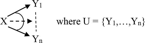
is a nonempty set of pairs of the form (X,U), so-called interactive forks, satisfying:
a)
and (possession of an absence value),b) for all
: , andc) for all (X,Ui),
: (disjointness of arcs).
Figure 13.Interactive fork (X,U).
3. (V,E,I) is called the interactive causal graph of the ICM.


Interactive (as well as conjunctive) causes are now relativized to sets Ui of effects. Variable X is called an interactive (conjunctive) cause simpliciter if X is an interactive (conjunctive) cause with respect to some Ui (these latter notions are no longer disjoint). For  a subset of variables of an interactive causal graph (V,E,I),
 denotes U’s subset of interactive causes in (V,E,I). The notion
 abbreviates the conjunction of the conditions
 for all
 (should I(U) be empty, the condition
 becomes vacuous). An interactive cause Z lies on a path π iff π carries
 ; that is, Z’s outgoing arrows on this path are connected by an arc (which may connect other effects), or formally, if for some
 ,
 with
 . A conjunctive cause Z lies on path π iff π carries
 and Z carries no arc; that is, there exists no
 with
 and
 . The other graph-theoretic notions remain unchanged.
Our notion of d*-connection exempts interactive causes from clause a:
(9) Definition: Two nodes X, Y of an interactive graph (V,E,I) are d*-connected given a set of nodes U iff they are connected by a path π in (V,E) such that
a) no intermediate cause or conjunctive common cause lying on π is in U, and
b) every common effect on π is in U or has an effect in U.
The next definition explicates the revised causal d*-connection condition. It consists of the minimal revision (i) together with the absence condition (ii):
(10) Definition: An ICM (V,E,I,P) satisfies the causal d*-connection condition C* iff for all X,  and
 :
i) if
, then X and Y are d*-connected given U, andii) if
, then X and Y are d-connected given U.


Axiom: Every physically possible system (V,E,P) that is [sufficiently] complete satisfies condition C*.
Observe that d-connection implies d*-connection, so if a CM satisfies C, it satisfies C*.
Condition 10.ii is equivalent to “if X and Y are d-separated given U, then  .” This condition breaks the symmetry between C and C*, but it is useful for the purpose of constructing a discovery algorithm for ICMs.
Condition C* is the revised global Markov condition. For finite acyclic ICMs C* is equivalent to a correspondingly revised local Markov condition M*. We say that Y is an interactive nonsuccessor of X if Y is neither an ordinary X successor nor a successor of a variable Z that is connected with X by an interactive arc:
(11) Definition: An ICM (V,E,I,P) satisfies the revised Markov condition M* iff every  is
i) independent of any subset of interactive nonsuccessors of X conditional on Par(X), and
ii) independent of any subset of (ordinary) nonsuccessors of X conditional on Par(X) and the condition
.

Theorem 1. For acyclic finite ICMs, conditions C* and M* are equivalent. (Proof omitted.)
The conditions of d*-faithfulness and d*-minimality are defined as follows:
(12) Definition:
1. An ICM (V,E,I,P) satisfies the condition of d*-faithfulness (F*) iff for all X,
and : if X and Y are d*-connected given U, then .2. A C*-satisfying ICM (V,E,I,P) satisfies the condition of d*-minimality (Min*) iff no arrow can be removed from E and no interactive fork from I without violating condition C*.


Axiom: Every physically possible C*-satisfying causal system satisfies Min*.
Axioms C* and Min* form the core of TCN*. Possible extensions are obtained by adding a cautious version of F* or condition T.
4. Conclusion and Outlook: The Discovery Problem for TCN*
In this article we argued that processes of indeterministic decay involve interactive causes. They violate the principle of “screening-off by common causes,” which is entailed by causal Markov condition, the core axiom of the theory of causal nets (TCN). We showed that there are interactive CMs that admit of no faithful noninteractive reconstruction. We developed a revised version the TCN, TCN*, that correctly predicts the probabilistic (in)dependencies of interactive CMs and coincides with TCN for CMs without interactive causes.
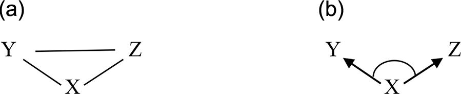
We cannot discuss the discovery problem for TCN*. Instead, we confine ourselves to brief observations. Recall the Spirtes et al. discovery algorithm for noninteractive CMs (Spirtes et al. Reference Spirtes, Glymour and Scheines1993, 114; Pearl Reference Pearl2000, 50): it first finds the unique undirected causal graph (assuming conditions C and F) and then orients some edges as common effects. We suggest that a revised discovery algorithm for ICMs can be obtained from the Spirtes et al. algorithm by adding a third step, roughly described as follows. For every undirected triangle (X,Y,Z) in the undirected graph and node X in this triangle, as in figure 14a, the algorithm checks whether an interactive cause interpretation of X is possible, as in figure 14b. This presupposes that (i) the absence condition holds ( and
 for some
 ) and (ii) edges between X, Y and neighboring nodes that have already been oriented are coherent with the nontransmission condition. The design of a revised discovery algorithm along these lines is a task for the future.
Additional discovery step for ICMs: Can an undirected triangle (a) be reconstructed as an interactive fork (b)?


 DEP(X,Y|Z)
 X→+Y
 X→+Z→−Y
 X→+/−Y
 X→Y
 par(Y)−{X}




 DEP(Y2,Y1|X)
 DEP(Y2,Z1|X)
 INDEP(Y2,Z1|X)