1 Introduction
The drop impact of a fluid onto a solid surface is an important phenomenon, largely studied in the literature. The complexity of this problem alone would be reason enough to investigate its multiple aspects. In addition, it has numerous applications in a myriad of industries, which also justifies facing the challenges associated with the understanding of this phenomenon. Common applications are inkjet printing, fire suppression, coating, food processing, painting, cleaning and chemicals in agriculture, among others. A rich variety of outcomes can be achieved by combinations of the impact velocity, the rheology of the drop fluid, the properties of the solid surface, and even the properties of the gas in which the process takes place. Depending on the kind of application, the purpose of the optimization can be very different. For example, there are some problems, such as the development of clothes that resist wetting (Bird, Dhiman & Varanasi Reference Bird, Dhiman and Varanasi2013), where it is desired to increase the probability of a drop’s rebounding after impact. On the other hand, when chemicals are being sprayed onto plants, efficiency is associated with the capacity of the drop to stick to the surface with which the drops are colliding (Wirth, Storp & Jacobsen Reference Wirth, Storp and Jacobsen1991), since less fluid is wasted and there is a decrease in the potential for toxic harm. A mapping of the diversity of results in terms of the different conditions of the process can provide valuable information that can be used to optimize the specific process.
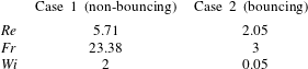
In the case of Newtonian fluids, the complexity generally comes from the interactions between inertial and capillary effects or between capillary and viscous effects, inducing regimes such as sticking, bouncing, spreading, receding and splashing (Yarin Reference Yarin2006). Low impact velocities induces the fluid to stick. High impact velocities induces the drop to spread up to a maximum diameter, after which the drop can either splash, when capillary forces are unable to guarantee the integrity of the drop, or to retract as a consequence of the stored energy in the interface. After retraction, the drop can bounce or oscillate in a damping motion towards an equilibrium shape (Bertola & Marengo Reference Bertola and Marengo2012). The usual dimensionless numbers that define the problem are the Froude (
 $Fr$
), Reynolds (
 $Re$
) and Webber (
 $We$
) numbers. Generally, the impact velocity is high when compared to the gravitational velocity
 $\sqrt{gL_{c}}$
and the Froude number is not considered. The
 $Re$
and
 $We$
are the most important dimensionless numbers from the time of impact until the point of maximum spreading, since kinetic energy is being dissipated or being transformed into surface tension energy. During the retraction stage, the capillary number (
 $Ca$
), which is a competition between viscous and interfacial effects (
 $We/Re$
), is more indicative.
As highlighted by Josserand & Thoroddsen (Reference Josserand and Thoroddsen2016), in practical applications most impacts are oblique. Even with its recognized importance, analyses of oblique drop impact are still scarce in the literature (Khojasteha et al.
Reference Khojasteha, Kazeroonib, Salariana and Kamalia2016). The large number of possible outcomes in this scenario are generally classified as (Antonini, Villa & Marengo Reference Antonini, Villa and Marengo2014): (i) deposition, which occurs when the drop sticks on the substrate; (ii) rivulet, which happens when the drop spreads downhill without recoiling; (iii) sliding, which takes place when the whole drop slides altogether downhill; (iv) rolling, when the drop rotates downhill from its point of contact; (v) partial rebound, which occurs when a portion of the drop rebounds, detaching itself from the rest of the drop, which remains stuck; and (vi) complete rebound, which takes place when the whole drop abandons the solid surface. As discussed by Yeong, Burton & Loth (Reference Yeong, Burton and Loth2014), the normal impact velocity is the best choice for the characteristic velocity employed to define the dimensionless numbers that correspond to those in the normal impact problem. They showed that a different set of stages happen, depending on whether the surface is ordinary or super-hydrophobic. Antonini et al. (Reference Antonini, Jung, Wetzel, Heer, Schoch, Moqaddam, Chikatamarla, Karlin, Marengo and Poulikakos2016) studied this problem from the experimental point of view and have shown that the Ohnesorge number,
 $Oh=\sqrt{Ca/Re}$
is the dimensionless parameter that can be correlated to the dynamics of no rebound – rebound scenarios. More particularly, in a Webber–Ohnesorge map,
 $Oh\approx 1$
delimits a boundary where
 $Oh<1$
shows a high correlation with a rebound response of the drop while
 $Oh>1$
shows a high correlation with a non-rebound response of the drop. Yeong et al. (Reference Yeong, Burton and Loth2014) corroborate these findings. Some other studies, (e.g Khojasteha et al.
Reference Khojasteha, Kazeroonib, Salariana and Kamalia2016), express their results with dimensional quantities, which sometimes can be more difficult to interpret.
Many applied problems, including fire suppression, inkjet printing and food processing, deal with the drop impact of non-Newtonian fluids. An additional motivation for studying the problem of the impact of a drop of a complex fluid is that small amounts of a solute can be used to obtain solutions with a desired non-Newtonian behaviour, which can optimize a certain kind of process (Bergeron et al. Reference Bergeron, Bonn, Martin and Vovelle2000; Bergeron Reference Bergeron2003). Depending on the character of the non-Newtonian fluid, very different outcomes can be expected. In the literature, we can find studies of specific classes of non-Newtonian fluids: shear-thinning fluids (German & Bertola Reference German and Bertola2009; An & Lee Reference An and Lee2012a ,Reference An and Lee b ; Bertola & Marengo Reference Bertola and Marengo2012), viscoelastic fluids (Bergeron et al. Reference Bergeron, Bonn, Martin and Vovelle2000; Rozhkov, Prunet-Foch & Vignes-Adler Reference Rozhkov, Prunet-Foch and Vignes-Adler2003; Bartolo et al. Reference Bartolo, Boudaoud, Narcy and Bonn2007; Smith & Bertola Reference Smith and Bertola2010; Bertola Reference Bertola2012; Izbassarov & Muradoglu Reference Izbassarov and Muradoglu2016), viscoplastic fluids and yield stress fluids.
There are few studies of the impact drops of fluids that exhibit a yield stress. Since they are the main focus of the present work, they need a more detailed analysis. For the reader who is not familiar with this class of fluids, we refer to the recent reviews of Balmforth, Frigaard & Ovarlez (Reference Balmforth, Frigaard and Ovarlez2014) and Bonn et al. (Reference Bonn, Denn, Berthier, Divoux and Manneville2017). The pioneering work on the subject was an experimental investigation conducted by Nigen (Reference Nigen2005) using a Vaseline lotion as the tested fluid and Plexiglass as the solid surface. In order to fit the obtained flow curve, a modified Cross model (that includes a yield stress parameter) was employed. The Bingham number (
 $Bn$
) was taken as the main dimensionless parameter for the study and it was found that for high
 $Bn$
(low impact velocities), there is a low spread due to the impact and the drop continues to spread in a creeping flow until reaching a maximum value, which is associated with the yield stress of the material. On the other hand, for low
 $Bn$
(high impact velocities), a higher maximum spreading was achieved just after impact, and the drop remained in that shape. Nigen (Reference Nigen2005) suggests that, unlike Newtonian fluids, the drop impact of yield stress fluids is more dominated by rheological effects than surface tension or other wetting properties. The work conducted by Luu & Forterre (Reference Luu and Forterre2009) using carbopol, bentonite and kaolin water solutions also showed that capillary forces were negligible. They concluded that the elastic character of these yield stress fluids does play an important role, not only before the stresses have reached the yield point state, but also beyond this limit. They analysed their experiments of drop impact from the perspective of the elasto-viscoplastic nature of a yield stress fluid without considering capillary forces, although these forces can be non-negligible in some situations. In this connection, Luu & Forterre (Reference Luu and Forterre2009) reported cases with rebound after retraction, which were attributed not to surface tension, but to the elastic character of the materials employed. It is worth noting that Coussot & Gaulard (Reference Coussot and Gaulard2005) concluded that the shape and size of an extruded yield stress material is given by a complex balance between gravity, the yield stress, and the extrusion speed, but does not involve the surface tension. The drop impact of a certain class of yield stress fluids was experimentally studied by German & Bertola (Reference German and Bertola2009) using solutions of a commercial polymer-based hairdressing gel whose flow curve is well fitted by a Herschel–Bulkley model. When the yield stress is low, they found similar results to those obtained with shear-thinning and Newtonian drops. However, for high values of the yield stress, the drop changes its shape during its trajectory towards the solid surface, with the lower portion of the drop (where stresses are higher) exhibiting a significant deformation while the upper portion remains un-deformed. This happened because the capillary length,
 $a\equiv \sqrt{\unicode[STIX]{x1D70E}/\unicode[STIX]{x1D70C}g}$
, was smaller than the initial radius of the drop. The shape of the drop before impact influences the dynamics of the impact of the drop and a fingerprint of this unusual result is that a disk-like shape is not obtained at maximum spread, instead central peaks are observed. Studying the effects of wettability, they found that no significant outputs were obtained when changing from a hydrophilic glass to a hydrophobic Parafilm substrate. Another experimental exploration of the drop impact of a yield stress fluid was conducted by Saidi, Martin & Magnin (Reference Saidi, Martin and Magnin2010). They explored the influence of the yield stress of Carbopol solutions, using a Herschel–Bulkley viscoplastic model to fit the flow curve. They found that for high impact velocities, the yield stress inhibits spreading and weakens retraction. Kim & Baek (Reference Kim and Baek2012) performed a numerical study of a viscoplastic material employing the Herschel–Bulkley equation for the flow curve and a generalized Newtonian fluid model in order to close the momentum equation. They studied the roles of the yield stress
 $\unicode[STIX]{x1D70F}_{y}$
, the consistency index
 $K$
, and the power-law index
 $n$
, independently. Kim & Baek (Reference Kim and Baek2012) found that increasing the yield stress in the viscoplastic drop did not change significantly the spreading stage, while the effect on the receding stage was in the direction of dampening the retraction. The effects of increasing
 $K$
and/or
 $n$
were to weaken both the spreading and receding stages. An interesting variant of the drop impact on a solid surface is the drop impact on a thin liquid layer of the same material, as explored by Blackwell et al. (Reference Blackwell, Deetjen, Gaudio and Ewoldt2015) for yield stress materials. In this case, the aspect ratio of the thickness of the layer to the diameter of the drop comes into play. They found that surface tension effects were also negligible, and that they could recover a number of results depending on the flow conditions of the problem. They developed an apparatus able to produce spherical-like drops, since this configuration is hard to obtain for a yield stress material from an extruded syringe process (German & Bertola Reference German and Bertola2009; Luu & Forterre Reference Luu and Forterre2009). Other variants of the problem include: when the drop is deposited on the surface, as explored by Jalaal, Balmforth & Stoeber (Reference Jalaal, Balmforth and Stoeber2015) investigating wall slip, or when the drop is launched onto another liquid (Cheng & Bertola Reference Cheng and Bertola2017; Jalaal, Kemper & Lohse Reference Jalaal, Kemper and Lohse2019). Uppal, Craster & Matar (Reference Uppal, Craster and Matar2017) investigated thixotropic effects in the spreading of a sessile drop. They used a very simplified model, where no elasticity and no yield stress effects are considered. Even so, they found that structural changes significantly influence the problem.
In the last decades, the numerical community has made a considerable effort to tackle the complexity of the impacting drop problem. In the confines of the Newtonian fluid, we can stress the recent discussions of the formation of dimples and the dynamics of splashing explored by Josserand & Thoroddsen (Reference Josserand and Thoroddsen2016), Philippi, Lagrée & Antkowiak (Reference Philippi, Lagrée and Antkowiak2016) and Jian et al. (Reference Jian, Josserand, Popinet, Ray and Zaleski2018), that were studied purely numerically. Non-Newtonian numerical simulations dealing with the phenomena of the impact of complex droplets are more commonly investigated employing viscoelastic models. Some examples along this line are: Fang et al. (Reference Fang, Owens, Tacher and Parriaux2006), which used an Oldroyd-B model and the smoothed particle hydrodynamics (SPH) method to handle the interface; Oishi et al. (Reference Oishi, Martins, Tome and Alves2012), which employed the eXtended Pom-Pom (XPP) model and the marker-and-cell method; Izbassarov & Muradoglu (Reference Izbassarov and Muradoglu2016), using the FENE-CR (Finite Extensible Nonlinear Elastic – Chilcott and Rallison) model and the volume of fluid method; and Wang, Do-Quang & Amberg (Reference Wang, Do-Quang and Amberg2017), who simulated the Giesekus model with a phase field method to track the interface. The literature on numerical predictions considering viscoplastic rheological models is scarcer. In particular, Kim & Baek (Reference Kim and Baek2012) employed a volume-of-fluid (VoF) method to study the impact dynamics of Herschel–Bulkley fluid droplets, and Noroozi, Tavangar & Hashemabadi (Reference Noroozi, Tavangar and Hashemabadi2013), also using the VoF method, investigated the Casson and Robertson-Stiff models in addition to the Herschel–Bulkley model, employing the open source code OpenFOAM and had, as their main focus, the shape of the viscoplastic drops.
In general, yield stress fluids are complex. In fact, viscoplastic models explore just a single aspect of this complexity, namely the role of the yield stress. In this regard, Bingham and Herschel–Bulkley models turn out to be incomplete tools for providing a thorough analysis of true yield stress fluids. However, in many experimental studies, the only rheological parameter that is considered is the yield stress. Although this analysis is useful, many papers dealing with general yield stress fluids have stressed the importance of other effects, such as elasticity and thixotropy (Balmforth et al. Reference Balmforth, Frigaard and Ovarlez2014; Coussot Reference Coussot2014; Bonn et al. Reference Bonn, Denn, Berthier, Divoux and Manneville2017), in many problems. As highlighted by Luu & Forterre (Reference Luu and Forterre2009), the elastic character of the yield stress fluid plays a crucial role in the drop impact problem and, therefore, they adopted an elasto-visoplastic model (Saramito Reference Saramito2007) as a way to explain their results. In addition, they call attention to the necessity of taking into account the thixotropic effects of the yield stress fluid. In very viscous fluids, as are most of the yield stress fluids, capillary forces and wettability properties play a less important role than the other rheological effects. Another fact worth noticing is that the receding dynamics in the Newtonian drop impact problem, which is governed by the elastic nature of the interfacial tension, have similar features to those of the retraction obtained from the elastic nature of yield stress fluids.
An additional aspect that deserves attention concerns the dimensionless numbers that govern the problem. Although the dimensionless numbers of the drop impact of yield stress fluids are most of the time listed in the papers that deal with drop impact, it is not uncommon to find in the literature results displayed as a function of a dimensional number, specially in experimental investigations. In this connection, we can find important investigations where the drop shapes are shown as a function of the impact velocity and/or yield stress. The reason for this happening seems to be the inherent difficulty of isolating the influence of a single dimensionless parameter by maintaining fixed all the remaining ones. This rationale is based on the fact that the impact velocity is the easiest variable to be changed in an experiment. Changing a property of the fluid or a geometric property, such as the diameter, is far more complicated, for obvious reasons. As an example, we can find in Nigen (Reference Nigen2005) an analysis that connects high impact velocity to low Bingham number and vice versa, when it seems to be desirable to decouple
 $Bn$
and
 $Re$
in order to capture the different aspects these dimensionless numbers are intended to represent. In a similar fashion, even if surface tension is not important, the Webber number is preferred to the Reynolds number for non-Newtonian drops for capturing the influence of the impact velocity. This seems to happen because the former does not take into account rheological parameters, i.e. unlike
 $Re$
,
 $We$
retains the same Newtonian expression. Another issue concerning dimensionless parameters is the recent discussion conducted by Thompson & Soares (Reference Thompson and Soares2016), where there is pointed out the importance of including the yield stress of the fluid in the formulation of the dimensionless numbers if viscous effects are to be taken into account. However, only one paper that deals with drop impact (Blackwell et al.
Reference Blackwell, Deetjen, Gaudio and Ewoldt2015) has recognized the importance of this fact, by a careful dimensionless analysis. As it will become clear, this dimensionless approach preserves the original viscoelastic properties of combinations between the Reynolds and Weissenberg numbers in the more general case of elasto-viscoplastic materials.
In the present paper, we investigate the normal and oblique drop impact problem for a yield stress fluid impacting on a solid surface, considering the elasto-viscoplastic thixotropic nature of this fluid. From the experimental studies of the drop impact of yield stress fluids, we can observe that the presence of a yield stress makes it probable that the problem operates within a range where capillary forces are negligible, i.e.
 $\unicode[STIX]{x1D70E}/D\ll \unicode[STIX]{x1D70F}_{c}$
, where
 $\unicode[STIX]{x1D70E}$
is the surface tension,
 $D$
is the diameter of the drop and
 $\unicode[STIX]{x1D70F}_{c}$
is a characteristic viscous stress, i.e. the shear stress evaluated at a characteristic shear rate. By construction
 $\unicode[STIX]{x1D70F}_{c}\geqslant \unicode[STIX]{x1D70F}_{y}$
. In addition, since some elastic effects due to capillary phenomenon can be reproduced by the elastic character of the material, this assumption can be considered a good approximation. Therefore, we neglect surface tension and contact line dynamics in the present analysis. The present method is not able to predict splashing or any rupture of the drop integrity. However, elastic forces are the ones that replace interfacial forces in order to inhibit drop rupture, and therefore, the presence of elasticity supports the assumption that there is no splashing. The impact shape of the drop can be a function of the balance of surface tension, gravity forces, and the yield stress at the moment of pinch-off at the nozzle. This fact leads to a shape dependency on the material and process properties. In addition, during the trajectory, this shape can experience changes. In order to promote a regular shape for comparison we assume that the drop has a circular shape during its trajectory to the substrate. Therefore, impact velocity merges in a unique manner initial velocity and height. This assumption can be reasonably reproduced in laboratory experiments by replacing the usual syringe by another method of producing a drop, such as the one presented in Blackwell et al. (Reference Blackwell, Deetjen, Gaudio and Ewoldt2015). A key ingredient of the present paper is the incorporation of thixotropic effects combined with other rheological features. The present paper uses a formulation developed in Oishi, Thompson & Martins (Reference Oishi, Thompson and Martins2016), Oishi, Martins & Thompson (Reference Oishi, Martins and Thompson2017), where a model for complex yield stress fluids, i.e. considering its elasto-viscoplastic thixotropic (EVPT) nature, is coupled to a marker-and-cell approach in order to handle free-surface problems. It is worth noting that the present investigation explores what was considered to be important further steps in the drop impact problem according to the guidelines stated by de Bruyn, Moyers Gonzalez & Frigaard (Reference de Bruyn, Moyers Gonzalez and Frigaard2016), who stressed the importance of the numerical simulation of yield stress fluids, Luu & Forterre (Reference Luu and Forterre2009), who highlighted the necessity of including thixotropic effects (in addition to elasticity), and Josserand & Thoroddsen (Reference Josserand and Thoroddsen2016), who called attention to the significance of considering the simulation of the oblique case.
2 Problem formulation
2.1 Geometry of the flow
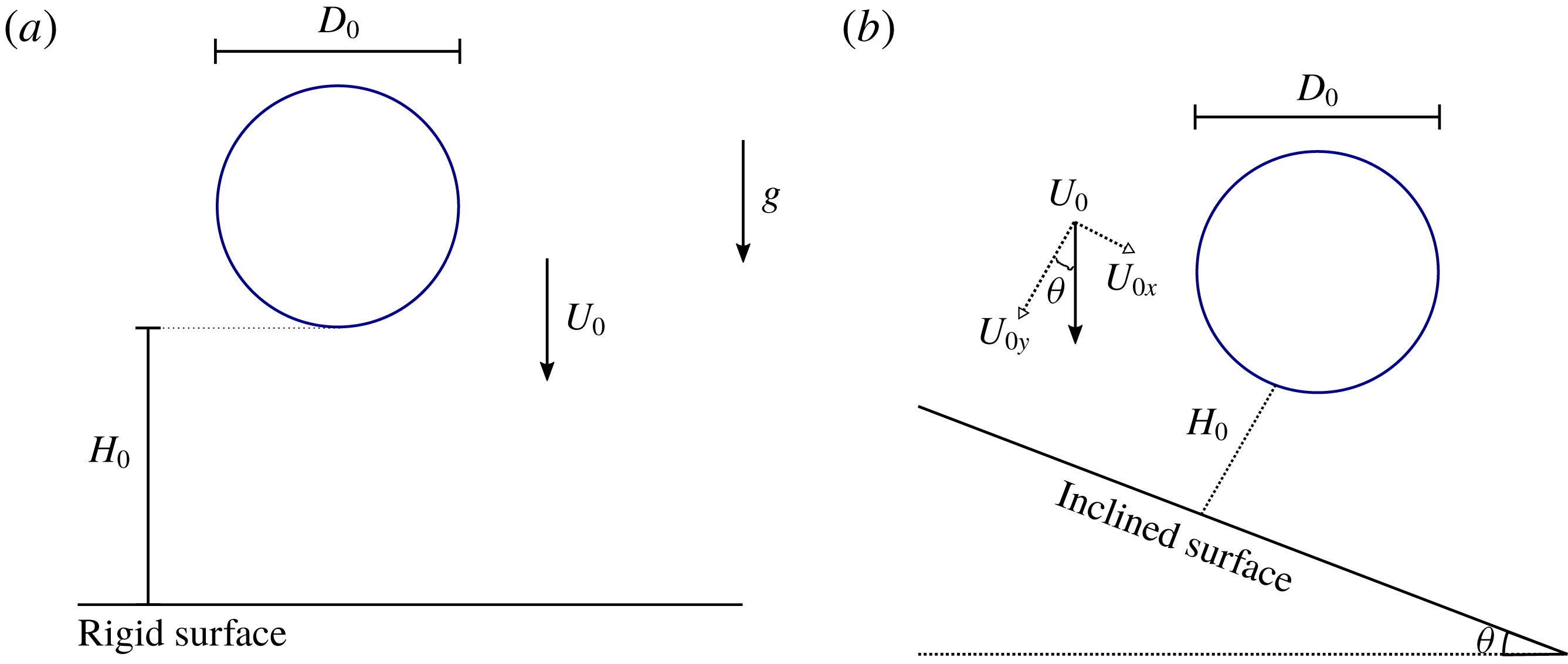
The problem of an impacting drop consists of a fluid drop launched with a velocity
 $U_{0}$
at a distance of
 $H_{0}$
from a rigid wall. In general, the normal impact velocity
 $U_{i}$
and the diameter
 $D_{0}$
of the drop are used in this problem to construct the dimensionless parameters, as will be presented in the next section. A scheme of the flow problem for the normal impact situation is illustrated in figure 1(a), while the drop impact on an inclined surface at a generic angle
 $\unicode[STIX]{x1D703}$
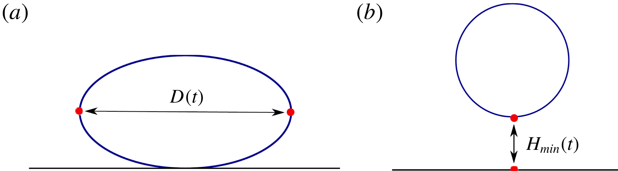
is sketched in figure 1(b). In the impacting drop problem, two important aspects analysed as time functions in the simulations/experiments are the spreading diameter
 $D(t)/D_{0}$
and the minimum bounce height
 $H(t)/D_{0}$
. These quantities are illustrated in figure 2.
Description of the flow problem: (a) normal drop impact and (b) impact on an inclined surface.

Illustration of the quantities: (a) the spreading diameter and (b) the minimum height of the drop.

In the present paper, we have fixed the drop diameter, for instance,
 $D_{0}=0.02$
m, based on the previous experimental work of Luu & Forterre (Reference Luu and Forterre2009) and Blackwell et al. (Reference Blackwell, Deetjen, Gaudio and Ewoldt2015).
The height of the drop from the plate is also fixed at
 $H_{0}=0.03$
m while the normal impact velocity is varied within the range
 $0.77~\text{m}~\text{s}^{-1}\leqslant U_{i}\leqslant 5.06~\text{m}~\text{s}^{-1}$
.
2.2 Physical guidelines
The model used in the present work can be seen as a generalization of the model for elasto-viscoplastic fluids of Saramito (Reference Saramito2007, Reference Saramito2009), but now accounting for thixotropic effects. There are two ways in which the model employed in the present work can be reduced to an elasto-viscoplastic model. One is to consider that quantities like viscosity and elastic modulus are still dependent on the structure parameter, but there is no delay between the current structure level and the equilibrium one. In other words, changes in stress induce instantaneous changes in structure impacting immediately the value of the mechanical properties. This first form is obtained by taking the limit where the thixotropic equilibrium time vanishes, i.e. when the time scale for structure changes is much shorter than the time scale of the considered processes. Another form of elasto-viscoplastic model is obtained in the other limit, when the material has constant mechanical properties that do not depend on the structure level. This second case is obtained by the model employed here by considering the limit where the thixotropic equilibrium time is very large, i.e. changes in structure are so slow that they do not happen in the time scales of the considered processes. Therefore, with respect to models for elasto-viscoplastic fluids, there is one phenomenon that is added, namely thixotropy, i.e. changes in the stress level have a finite time to impact the structure level. It is worth noticing that this additional phenomenon has influence on all the others since the mechanical properties of the material associated with elasticity and viscoplasticity are dependent on the structure parameter, whose changes are controlled by its degree of thixotropy. Therefore, a whole theory on how to introduce thixotropic effects is needed.
The general basis for the construction of a theory of how thixotropy affects the elasto-viscoplastic nature of the material is described in de Souza Mendes & Thompson (Reference de Souza Mendes and Thompson2012). Here, we highlight the main aspects. As commonly adopted in the literature, (e.g. Barnes Reference Barnes1997), a structure parameter
 $\unicode[STIX]{x1D706}\in [0,1]$
is the normalized quantity employed to describe the structural state of the material, where
 $\unicode[STIX]{x1D706}=0$
corresponds to the minimum structural level, and
 $\unicode[STIX]{x1D706}=1$
corresponds to the maximum structuring level. Making the mechanical properties functions of the structural state and applying an evolution equation for
 $\unicode[STIX]{x1D706}$
completes the backbone to taking into account thixotropic effects. The structural dependency of the viscosity and the elastic modulus of a viscoelastic model are defined so that the viscous and elastic effects are smaller in less structured states. The evolution equation depends on a driving potential between the current and the equilibrium structure states, where this last quantity is defined by the current stress level and by considering the flow curve as the locus of the attractor points corresponding to the equilibrium states. A breakdown process takes place only when the stress intensity surpasses the yield stress, providing the model with the main feature of a yield stress fluid.
2.3 The constitutive model
2.3.1 The total stress
The total stress is decomposed into three parts as
 $$\begin{eqnarray}\unicode[STIX]{x1D748}=-p\unicode[STIX]{x1D644}+\unicode[STIX]{x1D749}^{N}+\unicode[STIX]{x1D749}^{M},\end{eqnarray}$$
where
 $p$
is the pressure,
 $\unicode[STIX]{x1D749}^{N}=2\unicode[STIX]{x1D702}_{\infty }\unicode[STIX]{x1D63F}$
, where
 $\unicode[STIX]{x1D63F}$
is the rate of deformation tensor and
 $\unicode[STIX]{x1D702}_{\infty }$
is the viscosity related to the fully unstructured material. In addition,
 $\unicode[STIX]{x1D749}^{M}$
is a non-Newtonian part of the stress tensor that obeys an upper convected Maxwell equation of the following form
 $$\begin{eqnarray}\frac{\unicode[STIX]{x2202}\unicode[STIX]{x1D749}^{M}}{\unicode[STIX]{x2202}t}+\unicode[STIX]{x1D735}\boldsymbol{\cdot }(\boldsymbol{u}\unicode[STIX]{x1D749}^{M})-[(\unicode[STIX]{x1D735}\boldsymbol{u})\boldsymbol{\cdot }\unicode[STIX]{x1D749}^{M}+\unicode[STIX]{x1D749}^{M}\boldsymbol{\cdot }(\unicode[STIX]{x1D735}\boldsymbol{u})^{\text{T}}]=-\frac{G(\unicode[STIX]{x1D706})}{\unicode[STIX]{x1D702}(\unicode[STIX]{x1D706})}\unicode[STIX]{x1D749}^{M}+2G(\unicode[STIX]{x1D706})\unicode[STIX]{x1D63F},\end{eqnarray}$$
where
 $G(\unicode[STIX]{x1D706})$
and
 $\unicode[STIX]{x1D702}(\unicode[STIX]{x1D706})$
are the structure elastic modulus and structure viscosity. In the present work, the dependence of these material properties with respect to the structure parameter are given by
 $$\begin{eqnarray}\displaystyle & \displaystyle \unicode[STIX]{x1D702}(\unicode[STIX]{x1D706})=\left[\left(\frac{\unicode[STIX]{x1D702}_{0}}{\unicode[STIX]{x1D702}_{\infty }}\right)^{\unicode[STIX]{x1D706}}-1\right]\unicode[STIX]{x1D702}_{\infty }, & \displaystyle\end{eqnarray}$$
 $$\begin{eqnarray}\displaystyle & \displaystyle G(\unicode[STIX]{x1D706})=G_{0}\,f(\unicode[STIX]{x1D706})=G_{0}\exp \left[m\left(\frac{1}{\unicode[STIX]{x1D706}}-1\right)\right], & \displaystyle\end{eqnarray}$$
where
 $\unicode[STIX]{x1D702}_{0}$
and
 $G_{0}$
are the values of viscosity and elastic modulus in the fully structured state, respectively, and
 $m$
is a positive constant.
2.3.2 Evolution of the structure parameter
For the evolution for the structure parameter,
 $\unicode[STIX]{x1D706}$
, an additional equation is generally formulated specifying the rate of formation and rate of destruction of micro-structure. The following equation is obtained from simple assumptions in these terms with the stress being identified as the destructing agent, i.e.
 $$\begin{eqnarray}\frac{\unicode[STIX]{x2202}\unicode[STIX]{x1D706}}{\unicode[STIX]{x2202}t}+\unicode[STIX]{x1D735}\boldsymbol{\cdot }(\boldsymbol{u}\unicode[STIX]{x1D706})=\frac{1}{t_{eq}}\left(1-\frac{\unicode[STIX]{x1D706}}{\unicode[STIX]{x1D706}_{eq}(\unicode[STIX]{x1D70E})}\right),\end{eqnarray}$$
where
 $\unicode[STIX]{x1D706}_{eq}(\unicode[STIX]{x1D70E})$
is a function of the current stress intensity value. A fundamental concept of the determination of
 $\unicode[STIX]{x1D706}_{eq}(\unicode[STIX]{x1D70E})$
is the election of the flow curve as a set of steady-state points which is the locus of the attractor equilibrium points of the current non-equilibrium state. The thixotropic characteristic time,
 $t_{eq}$
, is the inverse of the rate of structure change in the state of maximum destruction. When
 $t_{eq}$
is high, thixotropic effects are more pronounced, i.e. a higher delay in structure change would occur as a consequence of a change in stress. Using the intensity of the deviatoric part of the stress tensor computed as
 $$\begin{eqnarray}\unicode[STIX]{x1D70E}_{dev}=\sqrt{{\textstyle \frac{1}{2}}\,\text{tr}\left[\left(\unicode[STIX]{x1D748}-{\textstyle \frac{1}{3}}\,\text{tr}(\unicode[STIX]{x1D748})\unicode[STIX]{x1D644}\right)^{2}\right]},\end{eqnarray}$$
and inputting this value in the flow curve, we can find an equilibrium deformation rate value,
 $\dot{\unicode[STIX]{x1D6FE}}_{eq}$
, corresponding to the current stress tensor. The equilibrium viscosity is computed by
 $$\begin{eqnarray}\unicode[STIX]{x1D702}_{eq}=\frac{\unicode[STIX]{x1D70E}_{dev}}{\dot{\unicode[STIX]{x1D6FE}}_{eq}}.\end{eqnarray}$$
Finally, we determine
 $\unicode[STIX]{x1D706}_{eq}(\unicode[STIX]{x1D70E}_{dev})$
corresponding to
 $\unicode[STIX]{x1D702}_{eq}$
. This structure parameter is obtained through the inverse of the viscosity function expressed by (2.3)
 $$\begin{eqnarray}\unicode[STIX]{x1D706}_{eq}=\frac{\ln \unicode[STIX]{x1D702}_{eq}-\ln \unicode[STIX]{x1D702}_{\infty }}{\ln \unicode[STIX]{x1D702}_{0}-\ln \unicode[STIX]{x1D702}_{\infty }}.\end{eqnarray}$$
The value of the current structure parameter that feeds (2.5) is computed by
 $$\begin{eqnarray}\unicode[STIX]{x1D706}=\frac{\ln [\unicode[STIX]{x1D702}(\unicode[STIX]{x1D706})+\unicode[STIX]{x1D702}_{\infty }]-\ln \unicode[STIX]{x1D702}_{\infty }}{\ln \unicode[STIX]{x1D702}_{0}-\ln \unicode[STIX]{x1D702}_{\infty }},\end{eqnarray}$$
where
 $$\begin{eqnarray}\unicode[STIX]{x1D702}(\unicode[STIX]{x1D706})+\unicode[STIX]{x1D702}_{\infty }=\frac{\unicode[STIX]{x1D70E}_{dev}}{\dot{\unicode[STIX]{x1D6FE}}}.\end{eqnarray}$$
2.3.3 Flow curve
The flow curve is generally obtained from a viscometric rheometry and constitutes a relation between the shear stress,
 $\unicode[STIX]{x1D70F}$
, and the deformation rate at steady-state conditions, i.e. equilibrium conditions. In the present work we will adopt the following equation that has shown to be useful in fitting rheometric data
 $$\begin{eqnarray}\unicode[STIX]{x1D70F}=\unicode[STIX]{x1D701}(\dot{\unicode[STIX]{x1D6FE}})(\unicode[STIX]{x1D70F}_{y}+K\dot{\unicode[STIX]{x1D6FE}}^{n})+\unicode[STIX]{x1D702}_{\infty }\dot{\unicode[STIX]{x1D6FE}},\end{eqnarray}$$
where
 $\unicode[STIX]{x1D70F}_{y}$
is the apparent yield stress of the material,
 $K$
and
 $n$
are the consistency and exponent of the power-law term in the flow curve, and
 $\unicode[STIX]{x1D702}_{\infty }$
is the viscosity at high shear rates. The function
 $\unicode[STIX]{x1D701}(\dot{\unicode[STIX]{x1D6FE}})$
is a regularization factor given by
 $$\begin{eqnarray}\unicode[STIX]{x1D701}(\dot{\unicode[STIX]{x1D6FE}})=\left\{\begin{array}{@{}ll@{}}1, & \text{if}~\unicode[STIX]{x1D70F}\geqslant \unicode[STIX]{x1D70F}_{y},\\ {\displaystyle \frac{(\unicode[STIX]{x1D702}_{0}-\unicode[STIX]{x1D702}_{\infty })\dot{\unicode[STIX]{x1D6FE}}}{\unicode[STIX]{x1D70F}_{y}+K\dot{\unicode[STIX]{x1D6FE}}^{n}}}, & \text{if}~\unicode[STIX]{x1D70F}<\unicode[STIX]{x1D70F}_{y},\end{array}\right.\end{eqnarray}$$
which is equivalent to considering a bi-viscosity model.
2.4 Governing equations and boundary conditions
For the isothermal motion of an incompressible material, the governing equations for mass and momentum are given by
 $$\begin{eqnarray}\displaystyle & \unicode[STIX]{x1D735}\boldsymbol{\cdot }\boldsymbol{u}=0, & \displaystyle\end{eqnarray}$$
 $$\begin{eqnarray}\displaystyle & \displaystyle \unicode[STIX]{x1D70C}\left[\frac{\unicode[STIX]{x2202}\boldsymbol{u}}{\unicode[STIX]{x2202}t}+\unicode[STIX]{x1D735}\boldsymbol{\cdot }(\boldsymbol{u}\boldsymbol{u})\right]=\unicode[STIX]{x1D735}\boldsymbol{\cdot }\unicode[STIX]{x1D748}+\unicode[STIX]{x1D70C}\boldsymbol{g}, & \displaystyle\end{eqnarray}$$
where
 $\unicode[STIX]{x1D748}$
is the total stress and
 $\boldsymbol{g}$
is the acceleration due to gravity.
The adopted boundary conditions for solving (2.13)–(2.14) are
 $$\begin{eqnarray}\boldsymbol{u}=\mathbf{0},\quad \text{on}~\unicode[STIX]{x2202}\unicode[STIX]{x1D6FA}_{d},\end{eqnarray}$$
and
 $$\begin{eqnarray}\unicode[STIX]{x1D748}\boldsymbol{\cdot }\boldsymbol{n}=\boldsymbol{t},\quad \text{on}~\unicode[STIX]{x2202}\unicode[STIX]{x1D6FA}_{t},\end{eqnarray}$$
where
 $\unicode[STIX]{x2202}\unicode[STIX]{x1D6FA}_{d}$
is the boundary where the velocity
 $\boldsymbol{u}$
is prescribed and
 $\unicode[STIX]{x2202}\unicode[STIX]{x1D6FA}_{t}$
is the domain boundary for imposing the traction condition. In (2.16),
 $\boldsymbol{n}$
denotes the outward unit normal vector to the boundary
 $\unicode[STIX]{x2202}\unicode[STIX]{x1D6FA}_{t}$
while
 $\boldsymbol{t}$
is the traction vector. From (2.16) we can obtain the normal stress and tangential stress boundary conditions, given by
 $$\begin{eqnarray}\displaystyle & \boldsymbol{n}\boldsymbol{\cdot }\unicode[STIX]{x1D748}\boldsymbol{\cdot }\boldsymbol{n}^{\text{T}}=\boldsymbol{n}\boldsymbol{\cdot }\boldsymbol{t}=F_{n},\quad \text{on}~\unicode[STIX]{x2202}\unicode[STIX]{x1D6FA}_{t}, & \displaystyle\end{eqnarray}$$
 $$\begin{eqnarray}\displaystyle & \boldsymbol{m}\boldsymbol{\cdot }\unicode[STIX]{x1D748}\boldsymbol{\cdot }\boldsymbol{n}^{\text{T}}=\boldsymbol{m}\boldsymbol{\cdot }\boldsymbol{t}=F_{m},\quad \text{on}~\unicode[STIX]{x2202}\unicode[STIX]{x1D6FA}_{t}, & \displaystyle\end{eqnarray}$$
where
 $\boldsymbol{m}$
is the unit tangent vector while
 $F_{n}$
and
 $F_{m}$
are known functions according to the physical problem which will be simulated.
For the structure parameter we solved (2.5) in
 $\unicode[STIX]{x2202}\unicode[STIX]{x1D6FA}_{t}$
whilst homogeneous Neumann boundary conditions are employed at the solid wall.
2.5 Dimensionless formulation
Due to the complexity of studying the combination of the rheological properties of an EVPT material and the flow properties of the impacting drop problem, it is convenient to describe the governing equations in a non-dimensional form. To begin with, we define the following dimensionless variables
 $$\begin{eqnarray}t^{\ast }=t\frac{U_{c}}{L_{c}},\quad \unicode[STIX]{x1D735}^{\ast }=L_{c}\unicode[STIX]{x1D735},\quad \boldsymbol{u}^{\ast }=\frac{\boldsymbol{u}}{U_{c}},\quad {\unicode[STIX]{x1D749}^{M}}^{\ast }=\frac{\unicode[STIX]{x1D749}^{M}}{\unicode[STIX]{x1D70F}_{c}},\quad p^{\ast }=\frac{p}{\unicode[STIX]{x1D70C}U_{c}^{2}},\quad \boldsymbol{g}^{\ast }=\frac{\boldsymbol{g}}{g},\quad \unicode[STIX]{x1D63F}^{\ast }=\unicode[STIX]{x1D63F}\frac{L_{c}}{U_{c}},\end{eqnarray}$$
where
 $t$
is the time,
 $\unicode[STIX]{x1D735}$
is the gradient operator,
 $\boldsymbol{u}$
is the velocity vector field. The characteristic stress
 $\unicode[STIX]{x1D70F}_{c}$
is defined (see Thompson & Soares Reference Thompson and Soares2016) by evaluating the stress in the non-regularized version of the extended Hershel–Bulkley model of (2.11). Therefore,
 $$\begin{eqnarray}\unicode[STIX]{x1D70F}_{c}=\unicode[STIX]{x1D70F}_{y}+K\left(\frac{U_{c}}{L_{c}}\right)^{n}+\unicode[STIX]{x1D702}_{\infty }\frac{U_{c}}{L_{c}},\end{eqnarray}$$
where the length and velocity scales
 $L_{c}$
, respectively,
 $U_{c}$
, are chosen to be the normal impact velocity
 $U_{i}$
, respectively, the drop diameter
 $D_{0}$
. Next, the dimensionless numbers related to the inertia, gravity, elasticity, plasticity and thixotropy of the fluid are defined by
 $$\begin{eqnarray}\left.\begin{array}{@{}c@{}}\displaystyle Re=\frac{\unicode[STIX]{x1D70C}U_{i}^{2}}{\unicode[STIX]{x1D70F}_{c}}~(\mathit{Reynold}\,\mathit{number}),\quad Fr=\frac{U_{i}}{\sqrt{gD_{0}}}~(\mathit{Froude}\,\mathit{number}),\\ \displaystyle \unicode[STIX]{x1D70F}_{y}^{\ast }=\frac{\unicode[STIX]{x1D70F}_{y}}{\unicode[STIX]{x1D70F}_{c}}~(\mathit{plastic}\,\mathit{number}),\\ \displaystyle Wi=\frac{\unicode[STIX]{x1D70F}_{c}}{G_{0}}~(\mathit{Weissenberg}\,\mathit{number}),\quad t_{eq}^{\ast }=t_{eq}U_{i}/D_{0}~(\mathit{Thixotropic}\,\mathit{number}),\end{array}\right\}\end{eqnarray}$$
Remark.
Note that (2.20) can be reformulated as
 $$\begin{eqnarray}1=\unicode[STIX]{x1D70F}_{y}^{\ast }+K^{\ast }+\unicode[STIX]{x1D702}_{\infty }^{\ast },\end{eqnarray}$$
where
 $$\begin{eqnarray}\unicode[STIX]{x1D70F}_{y}^{\ast }=\frac{\unicode[STIX]{x1D70F}_{y}}{\unicode[STIX]{x1D70F}_{c}},\quad K^{\ast }=\frac{K}{\unicode[STIX]{x1D70F}_{c}}\left(\frac{U_{c}}{L_{c}}\right)^{n},\quad \unicode[STIX]{x1D702}_{\infty }^{\ast }=\frac{\unicode[STIX]{x1D702}_{\infty }}{\unicode[STIX]{x1D702}_{c}},\end{eqnarray}$$
with the characteristic viscosity defined as
 $\unicode[STIX]{x1D702}_{c}\equiv \unicode[STIX]{x1D70F}_{c}L_{c}/U_{c}$
. Therefore, in the present model,
 $\unicode[STIX]{x1D702}_{\infty }^{\ast }$
denotes the unstructured dimensionless value of the viscosity, while the consistency index is denoted by
 $K^{\ast }$
.
At this point, it is important to notice that the arguments for choosing
 $\unicode[STIX]{x1D70F}_{c}$
as a characteristic viscous stress to compose the Reynolds number can be used to support the choice adopted for the Weissenberg number. This happens because the elastic Mach number,
 $M$
, that in viscoelastic fluids can be obtained from
 $M=\sqrt{Re\,Wi}$
can be computed by the same expression in elasto-viscoplastic fluids. The elastic number
 $El=Wi/Re$
is also embedded with the same physical meaning as conceived, if we adopt as a relaxation time
 $\unicode[STIX]{x1D702}_{c}/G_{0}$
.
Finally, omitting the asterisk, the system of equations for the incompressible and isothermal free surface flow used in the present paper is
 $$\begin{eqnarray}\displaystyle & \unicode[STIX]{x1D735}\boldsymbol{\cdot }\boldsymbol{u}=0,\qquad & \displaystyle\end{eqnarray}$$
 $$\begin{eqnarray}\displaystyle & \displaystyle \frac{\unicode[STIX]{x2202}\boldsymbol{u}}{\unicode[STIX]{x2202}t}+\unicode[STIX]{x1D735}\boldsymbol{\cdot }(\boldsymbol{u}\boldsymbol{u})=-\unicode[STIX]{x1D735}p+\frac{1}{Re}(\unicode[STIX]{x1D702}_{\infty }\unicode[STIX]{x1D6FB}^{2}\boldsymbol{u}+\unicode[STIX]{x1D735}\boldsymbol{\cdot }\unicode[STIX]{x1D749}^{M})+\frac{1}{Fr^{2}}\boldsymbol{g},\qquad & \displaystyle\end{eqnarray}$$
 $$\begin{eqnarray}\displaystyle & \displaystyle \frac{\unicode[STIX]{x2202}\unicode[STIX]{x1D749}^{M}}{\unicode[STIX]{x2202}t}+\unicode[STIX]{x1D735}\boldsymbol{\cdot }(\boldsymbol{u}\unicode[STIX]{x1D749}^{M})-[(\unicode[STIX]{x1D735}\boldsymbol{u})\boldsymbol{\cdot }\unicode[STIX]{x1D749}^{M}+\unicode[STIX]{x1D749}^{M}\boldsymbol{\cdot }(\unicode[STIX]{x1D735}\boldsymbol{u})^{\text{T}}]=\frac{f(\unicode[STIX]{x1D706})}{Wi}\left[-\frac{1}{\unicode[STIX]{x1D702}(\unicode[STIX]{x1D706})}\unicode[STIX]{x1D749}^{M}+2\unicode[STIX]{x1D63F}\right]\!.\qquad & \displaystyle\end{eqnarray}$$
As expected for a Weissenberg number,
 $Wi\rightarrow 0\Rightarrow \unicode[STIX]{x1D749}^{M}\rightarrow 2\unicode[STIX]{x1D702}(\unicode[STIX]{x1D706})\unicode[STIX]{x1D63F}$
, i.e. the fluid is purely viscous.
The form of the dimensionless equations associated with the evolution of the structure parameter, the mapping between viscosity and structure parameter (current and equilibrium ones), and the stress intensity, have exactly the same form as their dimensional counterparts.
The boundary conditions in dimensionless form are given by:
(i) No-slip boundary conditions
(2.27a,b ) $$\begin{eqnarray}u=0\quad \text{and}\quad v=0.\end{eqnarray}$$
(ii) Free surface stress conditions
(2.28)and$$\begin{eqnarray}\displaystyle & & \displaystyle -p+\frac{2\unicode[STIX]{x1D702}_{\infty }}{Re}\left[\frac{\unicode[STIX]{x2202}u}{\unicode[STIX]{x2202}x}n_{x}^{2}+\frac{\unicode[STIX]{x2202}v}{\unicode[STIX]{x2202}y}n_{y}^{2}+\left(\frac{\unicode[STIX]{x2202}u}{\unicode[STIX]{x2202}y}+\frac{\unicode[STIX]{x2202}v}{\unicode[STIX]{x2202}x}\right)n_{x}n_{y}\right]\nonumber\\ \displaystyle & & \displaystyle \quad +\,\frac{1}{Re}[(\unicode[STIX]{x1D70F}_{xx}^{M})n_{x}^{2}+2(\unicode[STIX]{x1D70F}_{xy}^{M})n_{x}n_{y}+(\unicode[STIX]{x1D70F}_{yy}^{M})n_{y}^{2}]=0;\end{eqnarray}$$
(2.29)where$$\begin{eqnarray}\displaystyle & & \displaystyle \frac{\unicode[STIX]{x1D702}_{\infty }}{Re}\left[2\frac{\unicode[STIX]{x2202}u}{\unicode[STIX]{x2202}x}n_{x}m_{x}+\frac{\unicode[STIX]{x2202}v}{\unicode[STIX]{x2202}y}n_{y}m_{y}+\left[\frac{\unicode[STIX]{x2202}u}{\unicode[STIX]{x2202}y}+\frac{\unicode[STIX]{x2202}v}{\unicode[STIX]{x2202}x}\right](n_{y}m_{x}+n_{x}m_{y})\right]\nonumber\\ \displaystyle & & \displaystyle \quad +\,\frac{1}{Re}[((\unicode[STIX]{x1D70F}_{xx}^{M})-(\unicode[STIX]{x1D70F}_{yy}^{M}))n_{x}n_{y}+(\unicode[STIX]{x1D70F}_{xy}^{M})(n_{y}^{2}-n_{x}^{2})]=0,\end{eqnarray}$$
$\boldsymbol{n}=(n_{x},n_{y})$
denotes the outward unit normal vector to the boundary while
$\boldsymbol{m}=(m_{x},m_{y})$
is the unit tangent vector.


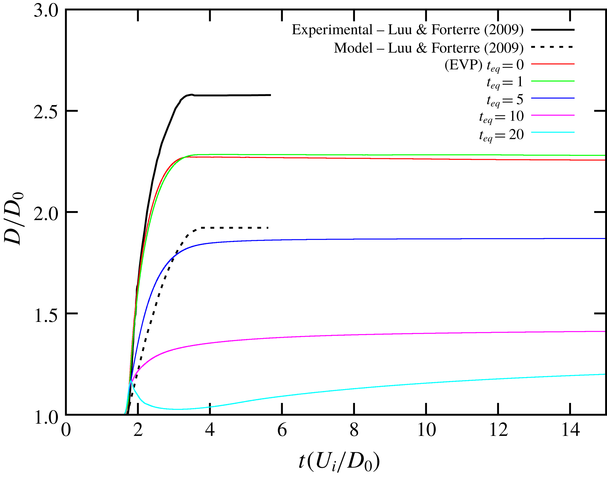
The elasto-viscoplastic thixotropic model of the present work is compared with the experimental and model results provided by Luu & Forterre (Reference Luu and Forterre2009) for the kaolin K51.

2.6 Overview of the computational technique
In this paper, we use a numerical scheme which combines the finite difference discretization and the marker-and-cell method implemented with in-house code. In summary, the two relevant stages of the numerical approach are as follows:
(i) Solving the governing equations. The conservation equations (2.24)–(2.25) are solved via a projection method which allows the solution in a segregated form. The constitutive equation (2.26) and the dimensionless counterpart of the evolution equation given by (2.5) are time discretized using the second-order Runge–Kutta scheme.
(ii) Moving free surface interface. In the context of the one-fluid model, the front-tracking method is employed here for dealing with the movement of the drop interface. The marker particles that describe the free surface are convected solving the equation
(2.30)$$\begin{eqnarray}\frac{\text{d}\boldsymbol{x}}{\text{d}t}=\boldsymbol{u}.\end{eqnarray}$$

More details about our code can be found in Oishi et al. (Reference Oishi, Thompson and Martins2016) while a mesh verification of the numerical scheme is presented in the appendix A.
3 Validation with experiments
In this section we performed numerical simulations in order to make comparisons with some experimental results provided by Luu & Forterre (Reference Luu and Forterre2009) and to validate our model and numerical approach.
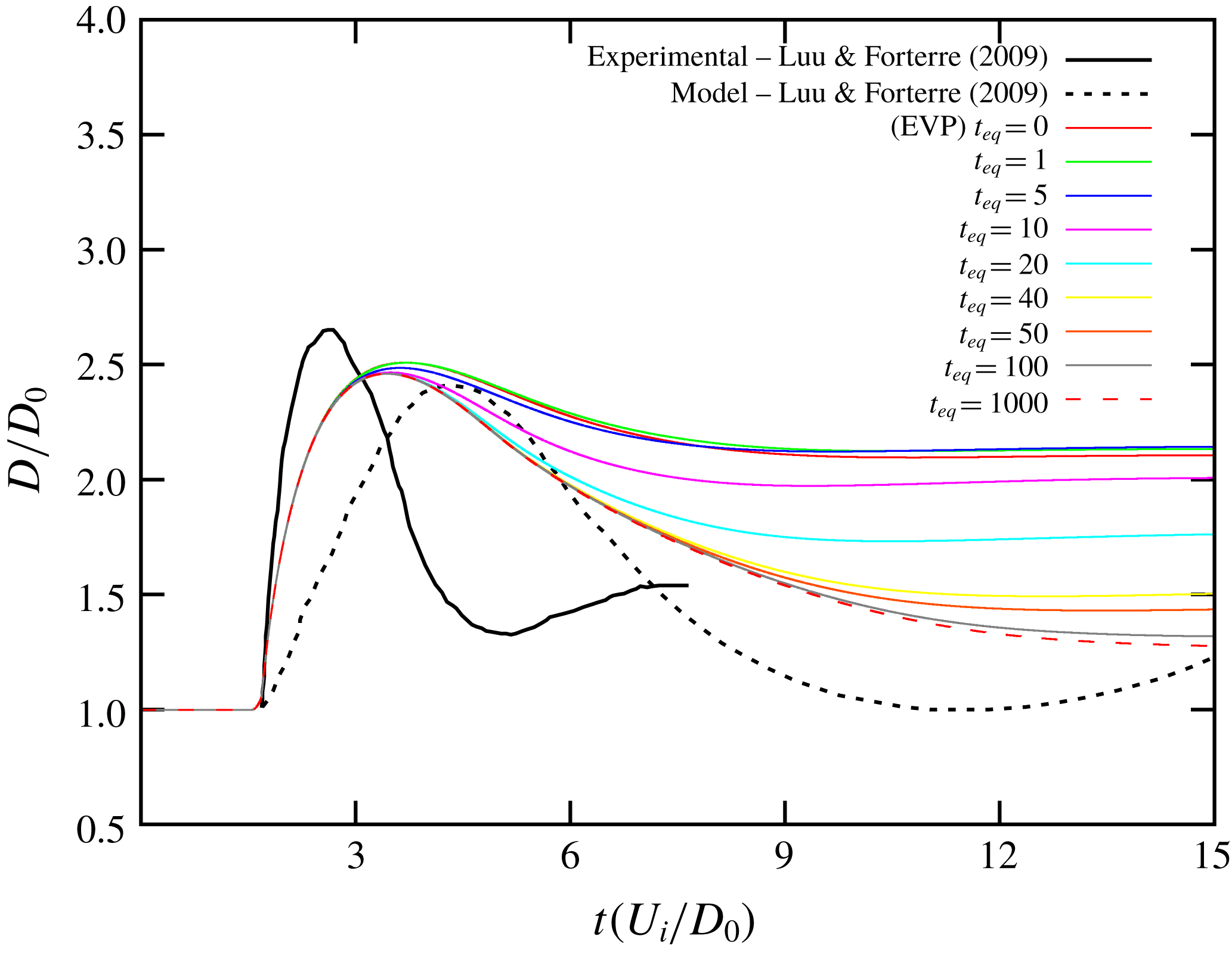
Figures 3 and 4 show the drop diameter evolution (see figure 2
a) obtained by the present model juxtaposed with the experimental and model results shown in Luu & Forterre (Reference Luu and Forterre2009) (see figure 10 of that paper). The parameters of the materials and process for both materials, kaolin K51 (51 % in weight of powder of kaolin added to de-ionized water) and carbopol C1, provided by Luu & Forterre (Reference Luu and Forterre2009) were introduced into our model. We tested some values for
 $t_{eq}$
corresponding to different levels of thixotropy. The qualitative behaviour of both materials was well captured by the present model. After achieving its maximum value, the diameter of the kaolin K51 drop exhibited a quite constant diameter behaviour while the carbopol C1 revealed a retraction. Concerning the response of the kaolin K51, low values of the thixotropic equilibrium time were able to improve the model prediction towards the experimental result, leading to a better performance than the one corresponding to the model employed by Luu & Forterre (Reference Luu and Forterre2009). It is worth noticing that when varying
 $t_{eq}$
, very different final diameter sizes were obtained. In the case of the carbopol C1, we can notice a small under-prediction of the size of the peak and an over-prediction of the time where it occurs, as well as lower retraction. However, compared with the model adopted by Luu & Forterre (Reference Luu and Forterre2009) the present model revealed a better performance also. Changes in
 $t_{eq}$
did not impact significantly the size and location in time of the peak, but lead to a variety of degrees of retractions. Different from the kaolin K51 response, the carbopol C1 was better captured for high values of the thixotropic equilibrium time. It is important to emphasize that the drop shape just before the moment of impact of the numerical approach is different from experimental one, as discussed previously.
The elasto-viscoplastic thixotropic model of the present work is compared with the experimental and model results provided by Luu & Forterre (Reference Luu and Forterre2009) for the carbopol C1.

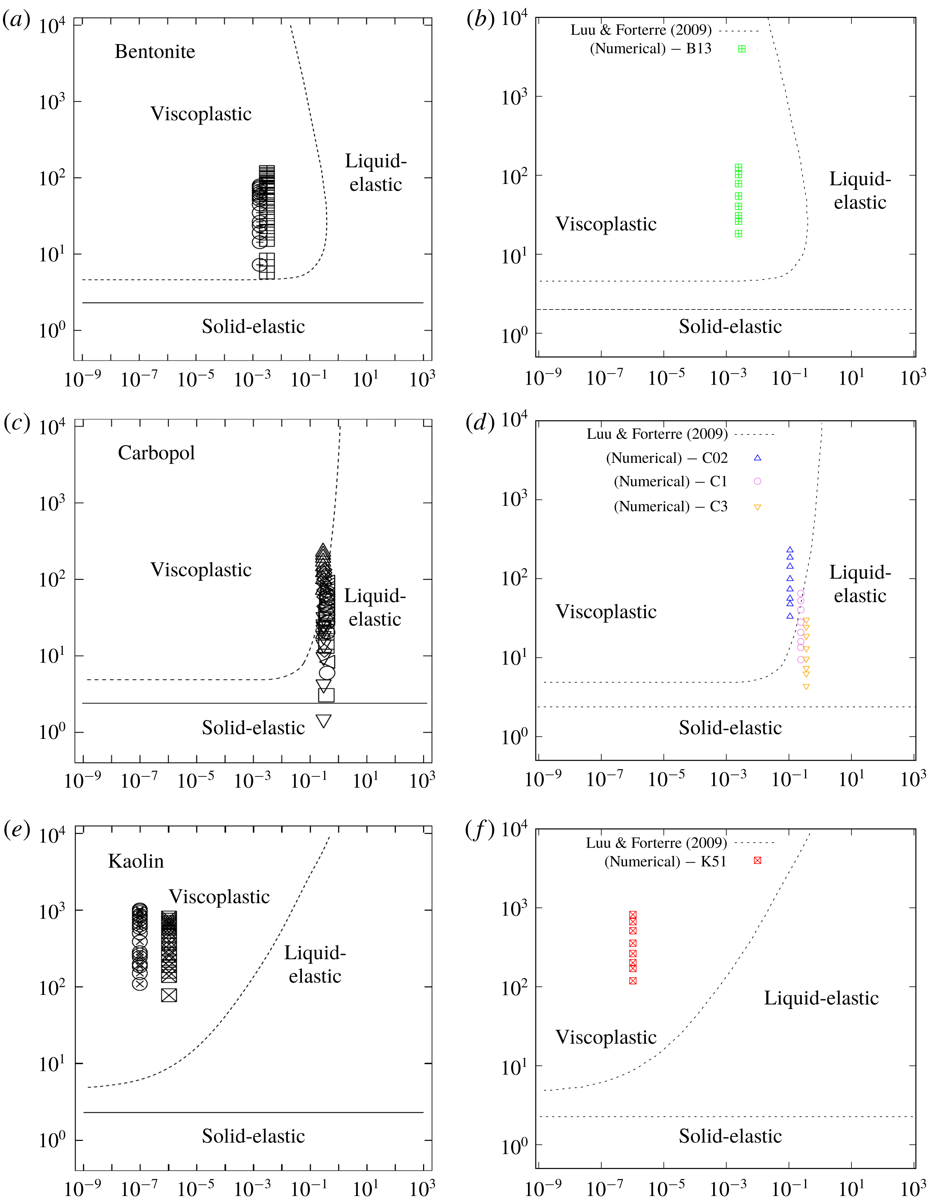
Parameters used in the numerical simulations (b,d,f) compared with those used in the experiments of Luu & Forterre (Reference Luu and Forterre2009) (a,c,e) in a map of
 $De/M$
versus
 $M/\unicode[STIX]{x1D6FE}_{y}$
. The dotted lines correspond to the different impact regimes predicted by Luu & Forterre (Reference Luu and Forterre2009). The points in the experimental maps show: (i) in the first row data for bentonite B13 and B15; (ii) in the second row data for carbopol C02, C035, C05, C1, C2, C3; (iii) in the third row data for kaolin K51 and K55. The numerical simulations of the present work were obtained for (i) in the first row, bentonite B13; (ii) in the second row carbopol C02, C1, C3; (iii) in the third row, kaolin K51.

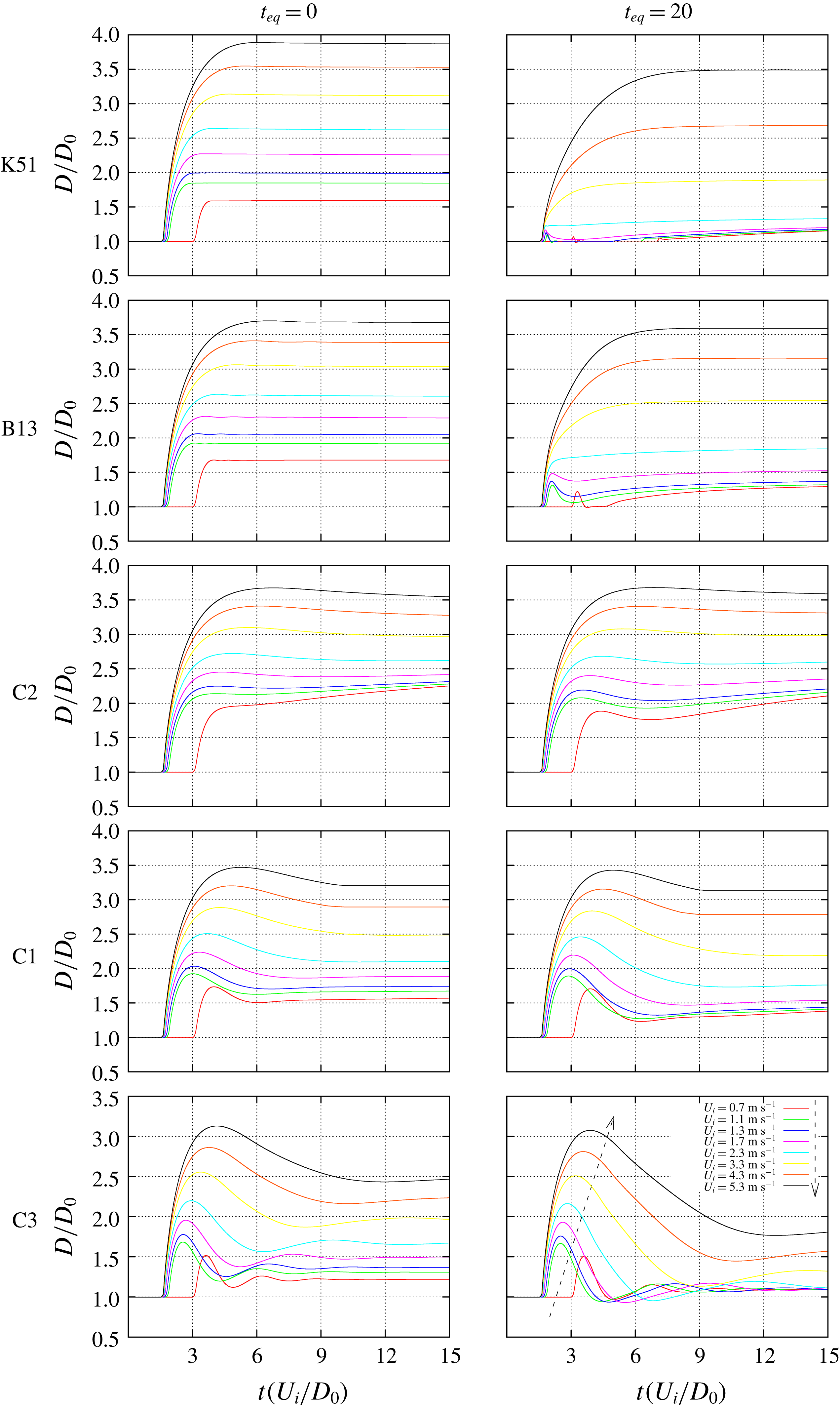
Dynamic response of the drop diameter of the cases shown in figure 5.

Another set of numerical results are compared with experimental data in figure 5. Our simulations using the mechanical properties of bentonite, B13 (13 % in weight of powder of bentonite added to de-ionized water), carbopol, C02, C1, and C3 (0.2 %, 1 %, 3 %, respectively, of mass concentration of carbopol), and kaolin (K51) for a number of impact velocities (figure 5
b,d,f) were compared with the experimental data obtained by Luu & Forterre (Reference Luu and Forterre2009) (a,c,e). The numerical simulations captured quite well the range explored by the experiments with the three materials. Figure 6 shows two different
 $t_{eq}$
-versions of the cases displayed in figure 5, since the analysis conducted by Luu & Forterre (Reference Luu and Forterre2009) did not consider thixotropic effects. In (a,c,e) we displayed the elasto-viscoplastic case of
 $t_{eq}=0$
, while in the (b,d,f), we show the case of
 $t_{eq}=20$
. The results for different velocities for the bentonite and the kaolin from (a,c,e) exhibited what was classified by Luu & Forterre (Reference Luu and Forterre2009) as a viscoplastic response, i.e. after achieving the maximum size, the drop diameter does not evolve. Therefore, the dynamic response obtained numerically is compatible with the experimental results. Timid oscillations can obtained for low velocities and
 $t_{eq}=20$
. In the carbopol material, increasing the concentration, we notice that a more elastic response is obtained. The results shown in figure 6 show a more viscoplastic response for lower concentrations (C02), while for high concentrations (C3) oscillatory responses are obtained. In this regard, the dynamic response of this material was also in accordance to the results shown by Luu & Forterre (Reference Luu and Forterre2009) where the border between viscoplastic and viscoelastic (called ‘liquid-elastic’ in that paper) responses was crossed.
In addition to thixotropy, the present model has some features that seem to be advantageous with respect to other elasto-viscoplastic models. The parameter
 $m$
present in the
 $G(\unicode[STIX]{x1D706})$
function provides a degree of elasticity when the stress is beyond the yield stress. Another feature is the use of the flow curve as the set of attractor points of the dynamic system where thixotropy induces non-equilibrium states.
There are a number of causes that can explain the differences between the present model and the experiments. First of all, the initial drop shape in the experiments are non-spherical in contrast to the numerical solution. Another source that can be important is related to extensional properties. The present model captures extensional effects in an indirect manner, i.e. with a relaxation characteristic time measured in shear. A different approach could be employed if there were extensional rheometric data. In addition, the elastic modulus adopted by Luu & Forterre (Reference Luu and Forterre2009) was, in fact, the storage modulus,
 $G^{\prime }$
, obtained from oscillatory experiments. These quantities are only related in the limit of linear viscoelasticity, which is defied in most of the experiments where deformation is by no means small.
The dimensionless numbers adopted to analyse the comparison between the present model and the experiments conducted by Luu & Forterre (Reference Luu and Forterre2009) were not adopted in the further analysis conducted here, since we find it appropriate to identify each case by the use of more primitive quantities that represent inertia, elasticity, plasticity and thixotropy.
4 Results: normal drop impact
In order to understand the complex interaction between the different phenomena that affect this problem, we will study the effect of the following dimensionless numbers:
 $Re$
,
 $Wi$
,
 $\unicode[STIX]{x1D70F}_{y}$
and
 $t_{eq}$
. In order to restrict the analysis to these four parameters, we keep fixed the Newtonian dimensionless term at
 $\unicode[STIX]{x1D702}_{\infty }=0.2$
. This means that changes in the plastic number are absorbed in the shear-thinning dimensionless term,
 $K$
. We mainly focus on three types of transient results: the minimum height; the spread factor; and the shape coloured by the structural level. As will become clear below, the first two parameters enable us to evaluate in the same picture the influence of three of the four dimensionless numbers analysed at a time. The evolution of the structure and shape can be illustrated by analysing the effects of two dimensionless numbers at a time.
4.1 Analysis of evolution of the height and diameter of the drop
Initially, we have concentrated our parametric studies on considering the influence of the elasticity, plasticity and inertia, fixing the thixotropic equilibrium time at
 $t_{eq}=7.5$
. The Weissenberg numbers have been selected to be
 $Wi=0.05$
, 0.5, 2, while the yield stress numbers have been selected to be
 $\unicode[STIX]{x1D70F}_{y}=0.1$
, 0.3, 0.5, 0.7. In the first round of simulations, we have considered lower normal impact velocities, which leads to the Reynolds numbers
 $Re=2.05$
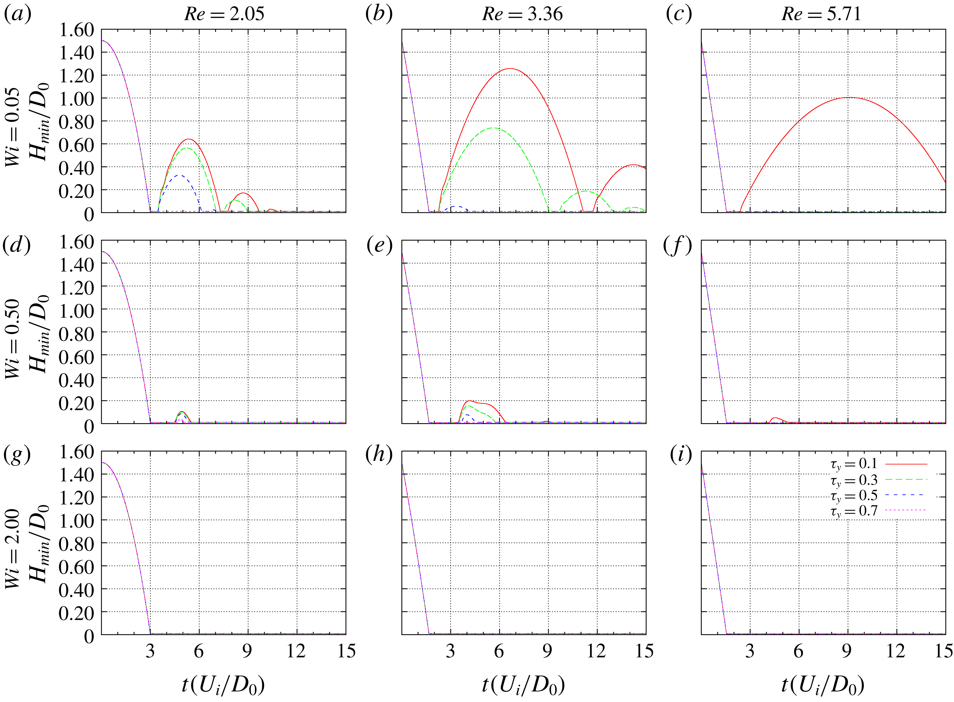
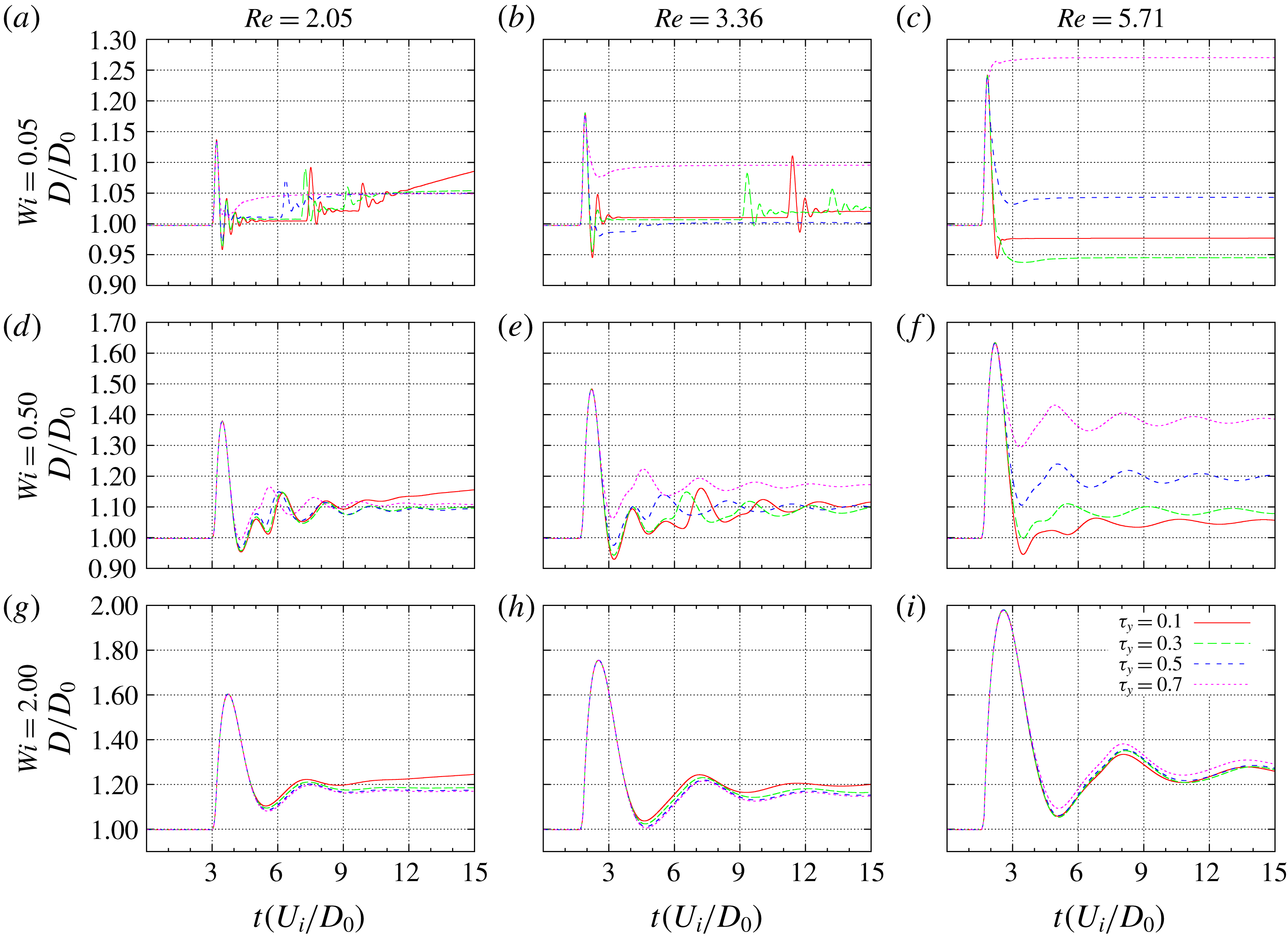
, 3.36, 5.71. The temporal evolution of the minimum height and the spread factor are presented in figures 7 and 8, respectively. The results are displayed in a Cartesian manner with the columns corresponding to different Reynolds numbers, while the rows correspond to the different Weissenberg numbers. The different curves inside each figure of
 $H(t)/D_{0}$
and
 $D(t)/D_{0}$
correspond to changes in the plastic number. This manner of displaying the results enables the reader to go from one subfigure to another by different paths, providing insights into the combined behaviour. The analysis conducted below does not cover the universe of all possibilities.
Temporal evolution of the normalized minimum bounce height
 $H(t)/D_{0}$
for
 $t_{eq}=7.5$
varying the following dimensionless parameters:
 $Wi=0.05$
, 0.5, 2 (rows),
 $Re=2.05$
, 3.36, 5.71 (columns) and
 $\unicode[STIX]{x1D70F}_{y}=0.1$
, 0.3, 0.5, 0.7 (inside of the figures).

Temporal evolution of the normalized drop diameter
 $D(t)/D_{0}$
for
 $t_{eq}=7.5$
varying the following dimensionless parameters:
 $Wi=0.05$
, 0.5, 2 (rows),
 $Re=2.05$
, 3.36, 5.71 (columns) and
 $\unicode[STIX]{x1D70F}_{y}=0.1$
, 0.3, 0.5, 0.7 (inside of the figures).

From figure 7 one can quickly get some rough information as to whether the drop bounces or not after the first impact. In this connection, we can see that increasing the Weissenberg number favours the scenario where the drop attaches to the floor. In the lowest row, corresponding to the highest Weissenberg numbers (
 $Wi=2$
), there are no situations where the drop bounces for the present value of
 $t_{eq}$
irrespective of the Reynolds or plastic numbers. From the results in the first row, we can see that the first rebound can achieve a significant height, especially for the lowest plastic number,
 $\unicode[STIX]{x1D70F}_{y}=0.1$
(red line). High values of
 $Wi$
imply high relative flexibility, hence, high elastic deformations. It is not a coincidence that the lowest row of the dual figure, figure 8, subfigures 8(g), 8(h) and 8(i), have higher maximum spreading factors when compared to their counterparts with lower Weissenberg numbers. The Reynolds number has a positive effect on the maximum spreading, due to the initial kinetic energy of the system, but the effect of the plastic number is low. Another major tendency that is shown in figure 7 is that increasing the plastic number also contributes to the absence of bouncing. It is tempting to attribute this to an increase in dissipation alone, which could rise due to an increase of the relative yield stress. However, because the plastic number only changes the balance with respect to the weights of yield stress, the power-law term, and the constant viscous term, perhaps another effect contributes to produce this result. In fact, from (2.26), we can see that the effective Weissenberg number,
 $Wi_{eff}(\unicode[STIX]{x1D706})\equiv Wi/f(\unicode[STIX]{x1D706})$
, is local and takes into account the structural level of the fluid at each point. Since lower values of the plastic number represent situations in which it is easier to break down the fluid, this induces higher values of the elastic modulus, which in turn lowers the effective Weissenberg number. As discussed previously, this favours bouncing at this level of
 $t_{eq}$
.
It is interesting to note that the influence of the Reynolds number is non-monotonic for
 $H(t)/D_{0}$
. Comparing subfigures 7(a), 7(b) and 7(c), we can see at least two effects that are worth mentioning. The first is that from
 $Re=2.05$
to 3.36, this low
 $Wi$
number produces opposite tendencies, depending on the plastic number. For example, this increase in
 $Re$
leads to stronger bouncing for low
 $\unicode[STIX]{x1D70F}_{y}$
(0.1 or 0.3), in the sense that the subsequent rebounds achieve a higher
 $H/D_{0}$
. On the other hand, for
 $\unicode[STIX]{x1D70F}_{y}=0.5$
, the same change in the Reynolds number leads to weaker bouncing. A second point worth noticing is the fact the top and the middle rows of figure 7 exhibit stronger bouncing at intermediate Reynolds numbers,
 $Re=3.36$
, when compared to
 $Re=2.05$
and 5.71 for the lower plastic number values
 $\unicode[STIX]{x1D70F}_{y}=0.1$
and 0.3. In other words, a non-monotonic effect is found for the increase of
 $Re$
. The increase in the kinetic energy that is gained from
 $Re=2.05$
to 3.36 is stored more as an elastic energy for lower values of
 $\unicode[STIX]{x1D70F}_{y}$
. However, a subsequent increase in the Reynolds number to
 $Re=5.71$
inhibits the bouncing of the fluids with different plastic number, so that the
 $\unicode[STIX]{x1D70F}_{y}=0.1$
case has a lower maximum height, while in the other cases there is no bouncing. These results can be explained by the following rationale. The energy per unit volume that is stored due to elastic effects is, roughly, given by
 $E_{el}=0.5\,G\unicode[STIX]{x1D6FE}_{e}^{2}$
, where
 $\unicode[STIX]{x1D6FE}_{e}$
is the elastic deformation. Lower values of the plastic number induces a higher elastic modulus and lower elastic deformation. With a small increase in the Reynolds number, the effect of increasing
 $G$
overcomes the decrease in the elastic deformation. With a higher increase in the Reynolds number, the breakdown process increases the dissipation and a smaller portion of the deformation is elastic.
From a general analysis of figure 8, we can observe that for most of the cases, the first spreading stage is not affected by the plastic number. This can be inferred by the spreading factor that, from the moment the drop reaches the floor until the moment where the maximum spreading factor is achieved, there is a coincidence among the different plastic number cases. The exception comes with higher values of the Reynolds and plastic numbers, where the drop spreads more intensively and the high value of the plastic number can prevent the receding stage (see the case where
 $\unicode[STIX]{x1D70F}_{y}=0.7$
in figure 8
c). In general, after achieving the maximum spreading factor, the receding stage starts with the different plastic number values still over the same master curve. Gradually, from the highest to the lowest plastic number value, the spreading factor curves abandon this master curve. This happens because higher values of the plastic number imply a higher resistance to receding, which inhibits the drop from returning to its original configuration. From figures 7(a) and 8(a) we can see that the different cases where bouncing occurs have similar contact times during the first contact period and that the spreading factors are also similar until the drop abandons the floor for the first time. Since the height achieved by the different fluids is not the same, this tendency does not happen for subsequent rebounds. In fact, we can see a decrease in the number of rebounds in this case of low
 $Re$
and low
 $Wi$
: three for
 $\unicode[STIX]{x1D70F}_{y}=0.1$
, two for
 $\unicode[STIX]{x1D70F}_{y}=0.3$
, one for
 $\unicode[STIX]{x1D70F}_{y}=0.5$
and zero for
 $\unicode[STIX]{x1D70F}_{y}=0.7$
. The effect of the plastic number on the spreading factor is monotonic and well defined in the
 $Wi=0.5$
–
 $Re=5.71$
case, where a clear separation between the curves occurs after the maximum spreading. The higher resistance of fluids with higher plastic numbers leads to oscillations at the floor around larger diameters. When the Weissenberg number is increased, the plastic number has a weak effect, showing that elasticity damps the effect of the yield stress. For the lowest
 $Wi$
, keeping
 $Re=5.71$
, we can see a decrease in the tendency of an oscillatory motion. The non-monotonic result of the case of the lowest plastic number can be attributed to the bouncing of this drop during the captured period. These general results are in accordance with some experimental data provided by Luu & Forterre (Reference Luu and Forterre2009), where the elastic character of the yield stress fluid mimics some of the results obtained by inelastic fluids where interfacial effects have an elastic nature.
The effects of thixotropy, combined with elasticity, and inertia are analysed considering a high value of the plastic number,
 $\unicode[STIX]{x1D70F}_{y}=0.7$
, shown in figures 9 and 10 for minimum height and spreading factor, respectively. For these investigations, we have taken various Weissenberg numbers,
 $Wi=0.05$
, 0.5, 2, various Reynolds numbers,
 $Re=2.05$
, 5.71, 13.49, and various thixotropic equilibrium times,
 $t_{eq}=5$
, 7.5, 10, 20.
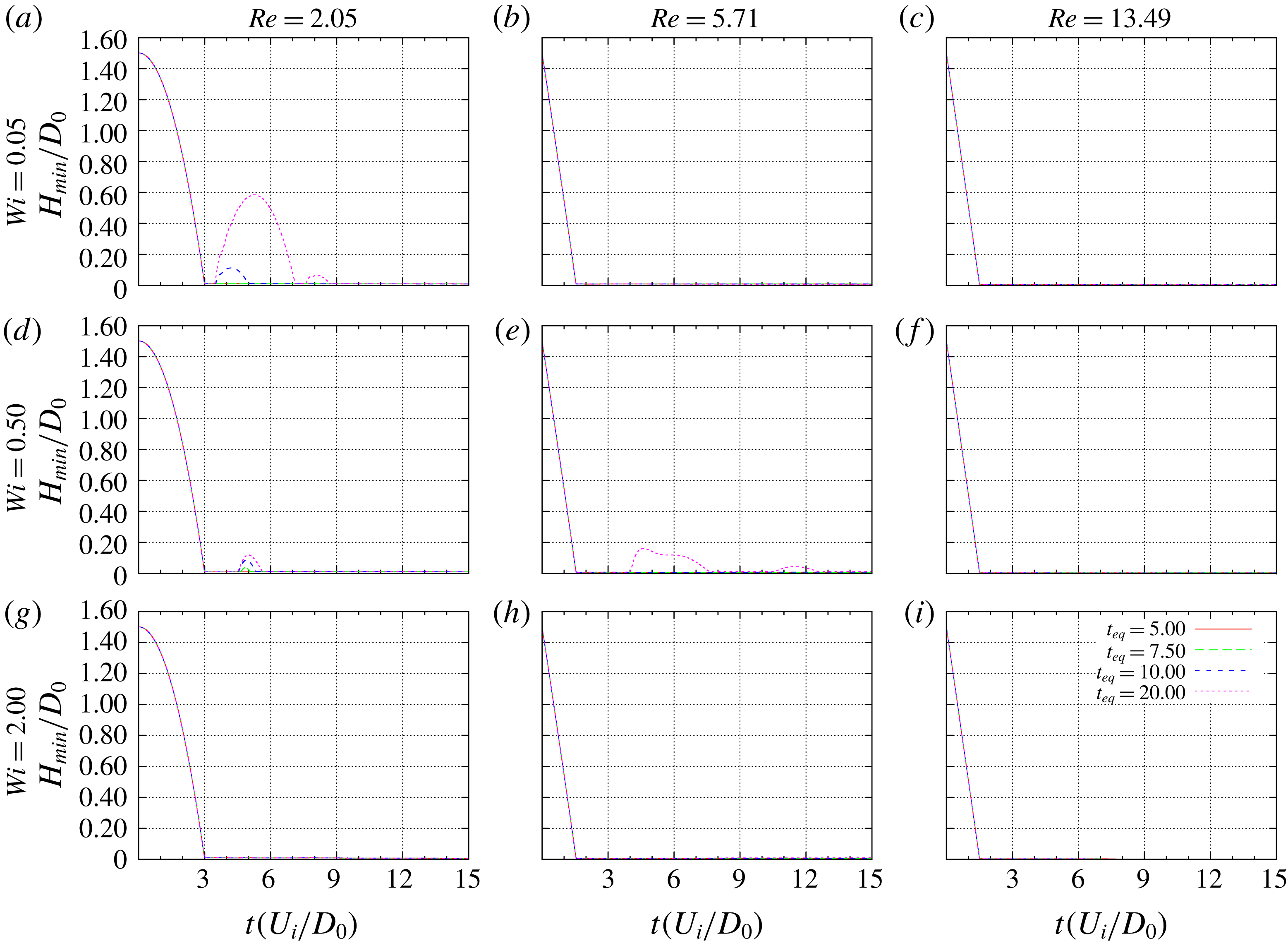
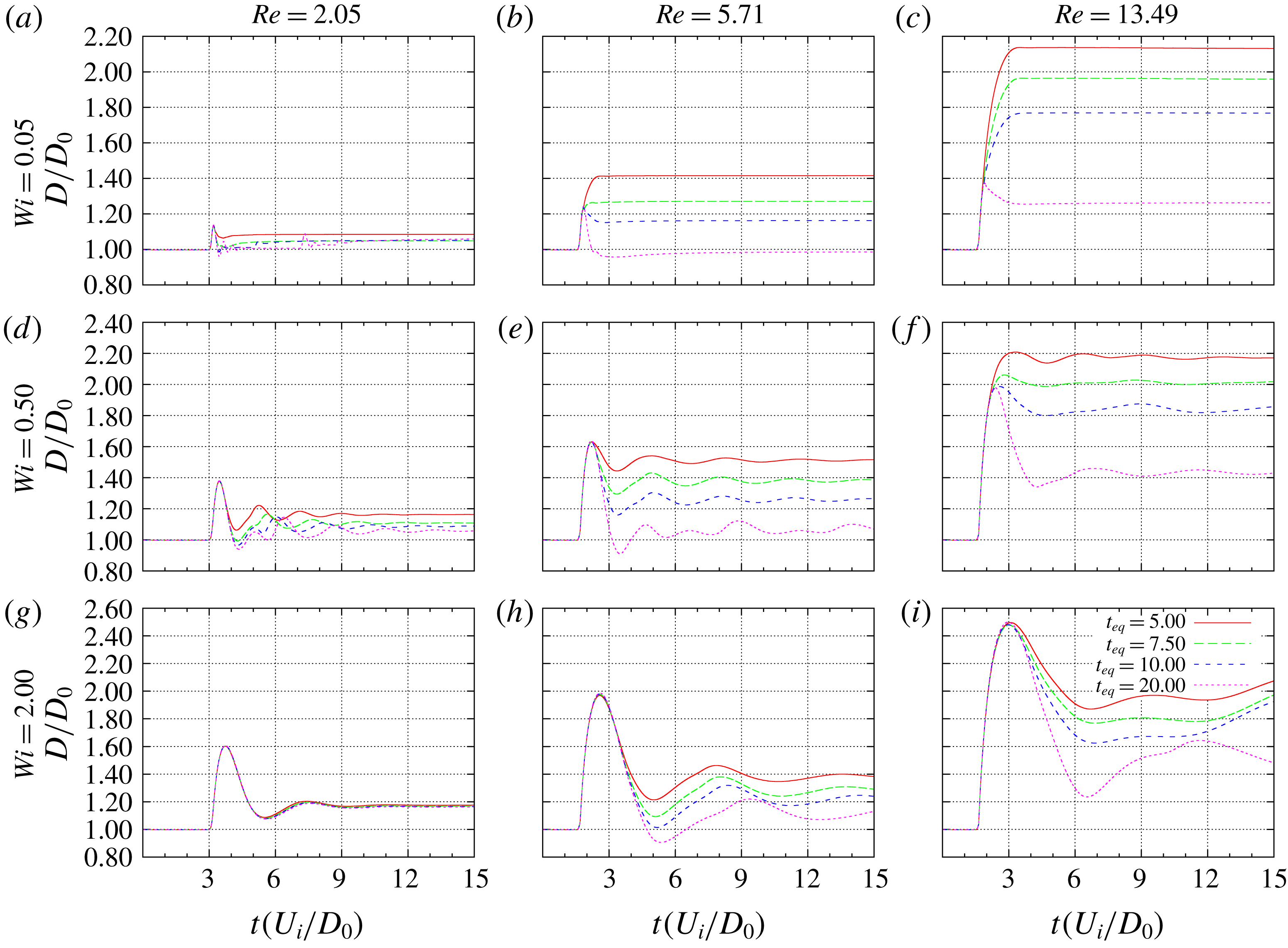
The first thing that attracts attention when one examines figure 9 is that there are few cases with rebounds. However, this high a value of the plastic number inhibits rejuvenation, which in turn keeps the level of elasticity high. In the material analysed in the present paper, this implies higher elastic deformations, which can be verified from the levels of the spreading factor depicted in figure 10, which exceed significantly those obtained in when
 $\unicode[STIX]{x1D70F}_{y}=0.1$
(not shown here). The few bouncing results are associated to high values of
 $t_{eq}$
, as discussed previously. When there is not enough time for the structure to change, the drop kicks just after it impacts the solid surface, as an elastic ball.
The lower
 $Wi$
row shows almost non-oscillating results. As the Reynolds number is increased, gradually the final configuration is changed from the maximum to the minimum spreading factor, since lower thixotropic equilibrium times induce the drop to remain at the maximum relative diameter, while higher values of
 $t_{eq}$
enable the fluid to retract; but once the minimum spreading factor is achieved, there is not enough energy to overcome the yield threshold. The intermediate Weissenberg number row is just a wavy version of the top row, where now elastic effects are able to induce oscillations in the drop. The case of high
 $Wi$
, high Reynolds number, and high
 $t_{eq}$
shows the beginning of nonlinear combinations of elastic, inertial and thixotropic effects.
Temporal evolution of the normalized minimum bounce height
 $H(t)/D_{0}$
for
 $\unicode[STIX]{x1D70F}_{y}=0.7$
, varying the following dimensionless parameters:
 $Wi=0.05$
, 0.5, 2 (rows),
 $Re=2.05$
, 5.71, 13.49 (columns) and
 $t_{eq}=5$
, 7.5, 10, 20 (inside of the figures).

Temporal evolution of the normalized drop diameter
 $D(t)/D_{0}$
for
 $\unicode[STIX]{x1D70F}_{y}=0.7$
, varying the following dimensionless parameters:
 $Wi=0.05$
, 0.5, 2 (rows),
 $Re=2.05$
, 5.71, 13.49 (columns) and
 $t_{eq}=5$
, 7.5, 10, 20 (inside of the figures).

4.2 Bouncing–non-bouncing outputs of the normal drop impact
A qualitative aspect of the problem that is of particular practical importance in the drop impact problem is if the drop will bounce or stick in the substrate. In order to reduce the four-dimensional parameter space of the dimensionless numbers analysed in this work, we followed the rationale described next.
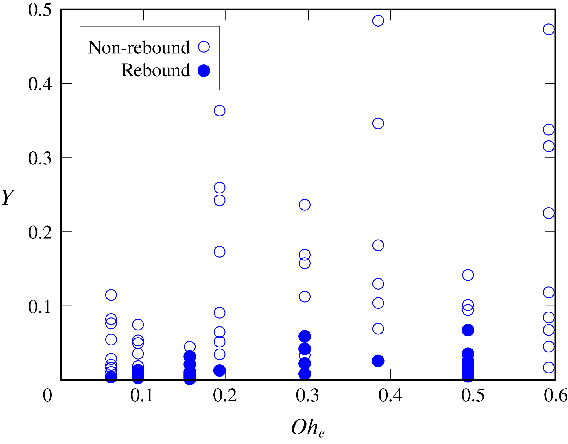
Considering that the elasticity of the material is responsible for effects that in the Newtonian case are attributed to elastic interfacial causes, we can apply what was learned from the literature and elect a counterpart of the Ohnesorge number as a parameter to be analysed. From its original definition an elastic Ohnesorge number can be defined as
 $Oh_{e}\equiv \sqrt{Wi/Re}$
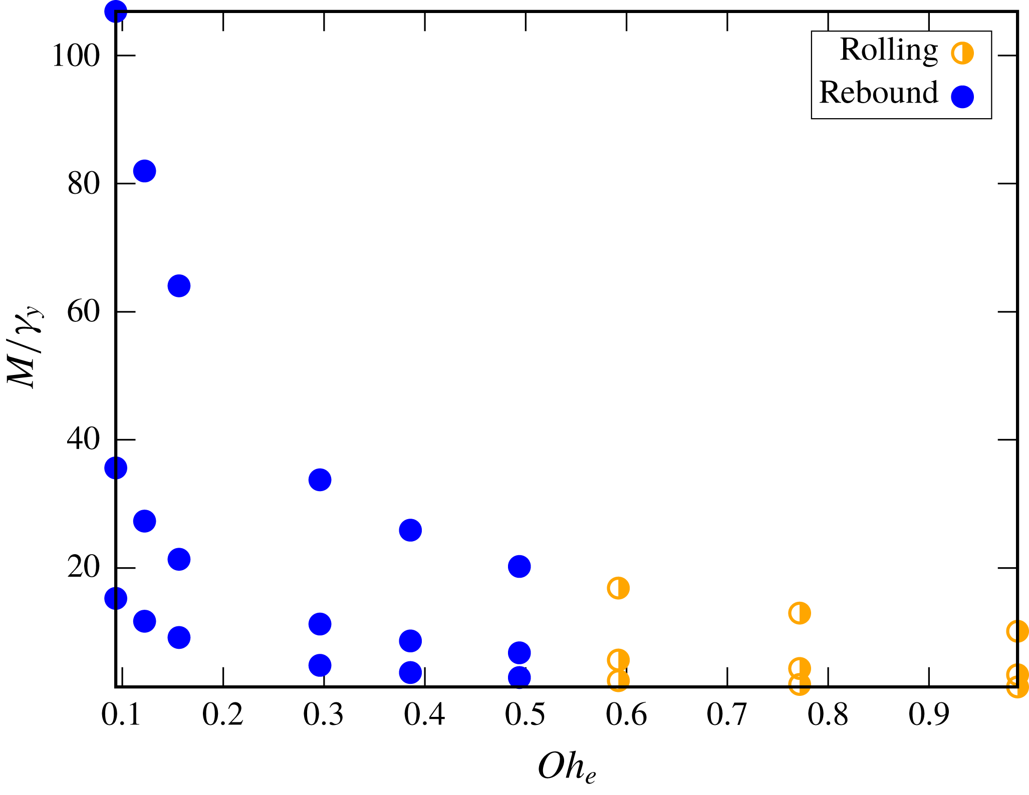
, which preserves a lack of dependence with the characteristic velocity. A second combination of dimensionless numbers is obtained from the observation of the results described in the previous subsection. For the range of the tested parameters, we could identify a non-bouncing tendency when
 $Re$
,
 $Wi$
and
 $\unicode[STIX]{x1D70F}_{y}$
are increased. The opposite trend would happen by increasing
 $t_{eq}$
. The importance of the elastic Mach number,
 $M\equiv U/\sqrt{G/\unicode[STIX]{x1D70C}}=\sqrt{Wi\,Re}$
, highlighted in Luu & Forterre (Reference Luu and Forterre2009), lead us to construct the following dimensionless number
 $$\begin{eqnarray}Y=\frac{M\unicode[STIX]{x1D70F}_{y}}{t_{eq}}.\end{eqnarray}$$
The ratio
 $\unicode[STIX]{x1D70F}_{y}/t_{eq}$
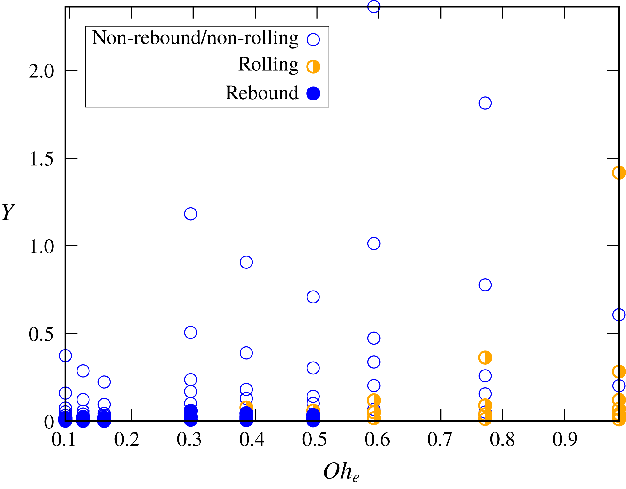
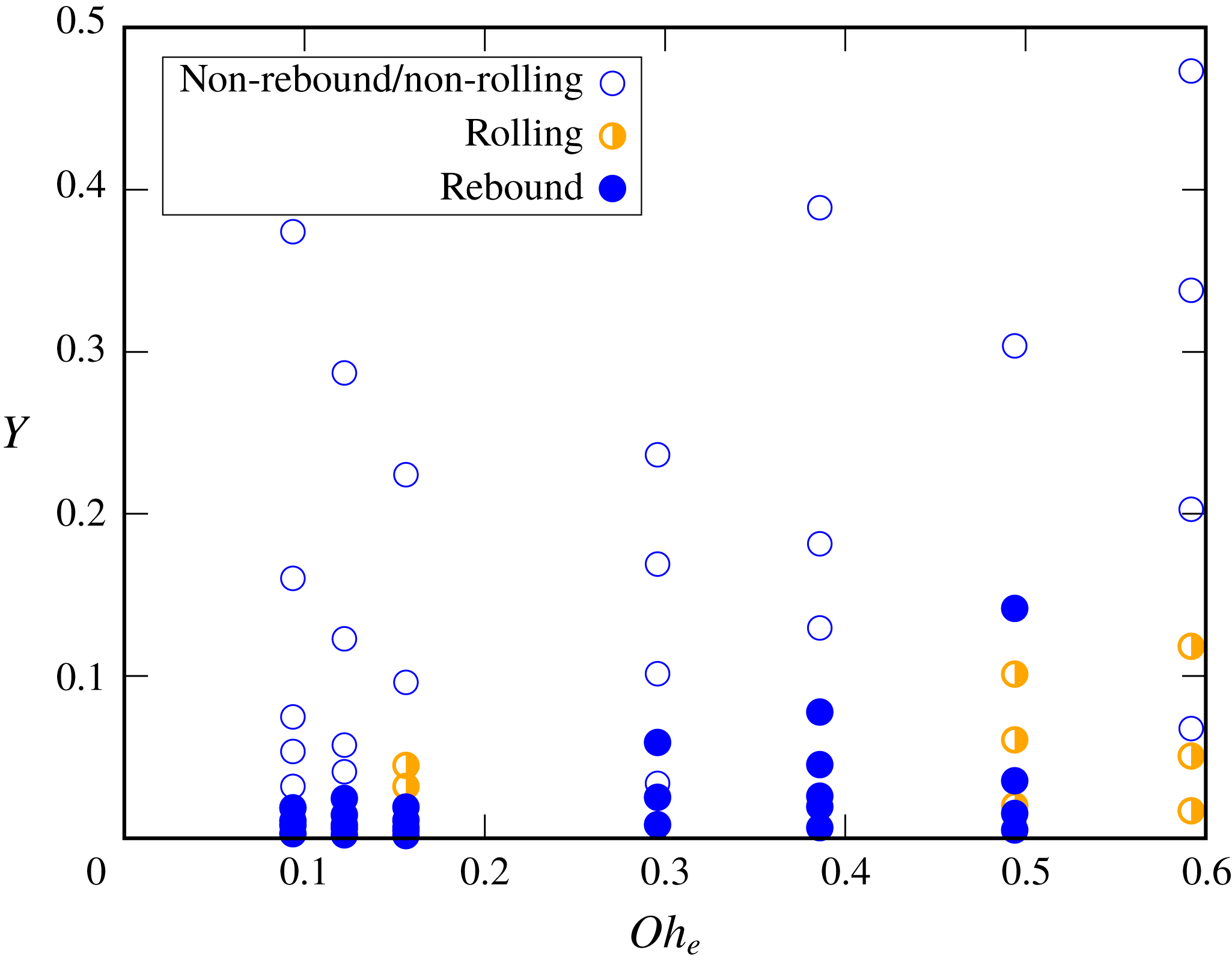
can be interpreted as a dissipation per unit volume due to the plastic nature of the material during a time scale equivalent to the thixotropic equilibrium time of the material. Therefore, it is reasonable to expect that increasing this ratio, the material has a tendency to avoid bouncing. In figure 11, we can see a plot of
 $Y$
versus
 $Oh_{e}$
for the normal impact case. Rebound and non-rebound outputs were separated, although not perfectly. A critical value for the elastic Ohnesorge number was identified, i.e. for
 $Oh_{ec}>0.5$
no bouncing occurred (results for higher
 $Oh_{e}$
values not shown in this figure corroborate this finding). For
 $Y>\approx 0.08$
no bouncing results are verified, but we can identify some non-bouncing results below this value. In the appendix B, we provide maps of the bouncing–non-bouncing outputs for the four dimensionless numbers analysed in the present work.
Normal impact.

4.3 Analysis of the evolution of the shape and structure of the drop
The last set of results of the normal drop impact subsection are some selected cases that show the temporal evolution of the position and shape of the drops, filled with the structure parameter field,
 $\unicode[STIX]{x1D706}$
. The
 $\unicode[STIX]{x1D706}$
domain,
 $\unicode[STIX]{x1D706}\in [0,1]$
, was divided equally into seven parts and a different colour was designated for each part. The colours range from dark blue (corresponding to the lowest values of
 $\unicode[STIX]{x1D706}$
) to a yellow mustard colour (corresponding to the highest values of
 $\unicode[STIX]{x1D706}$
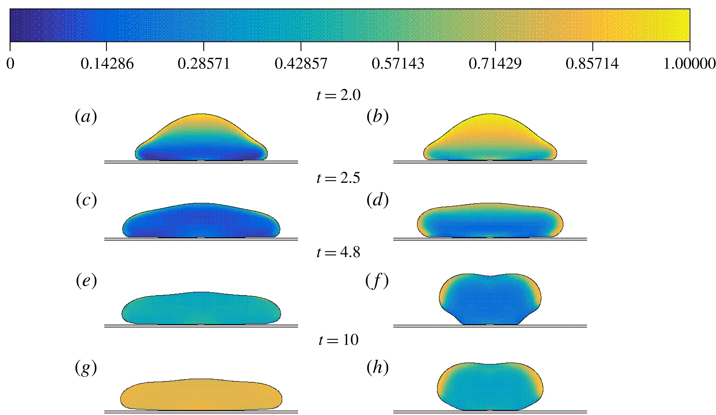
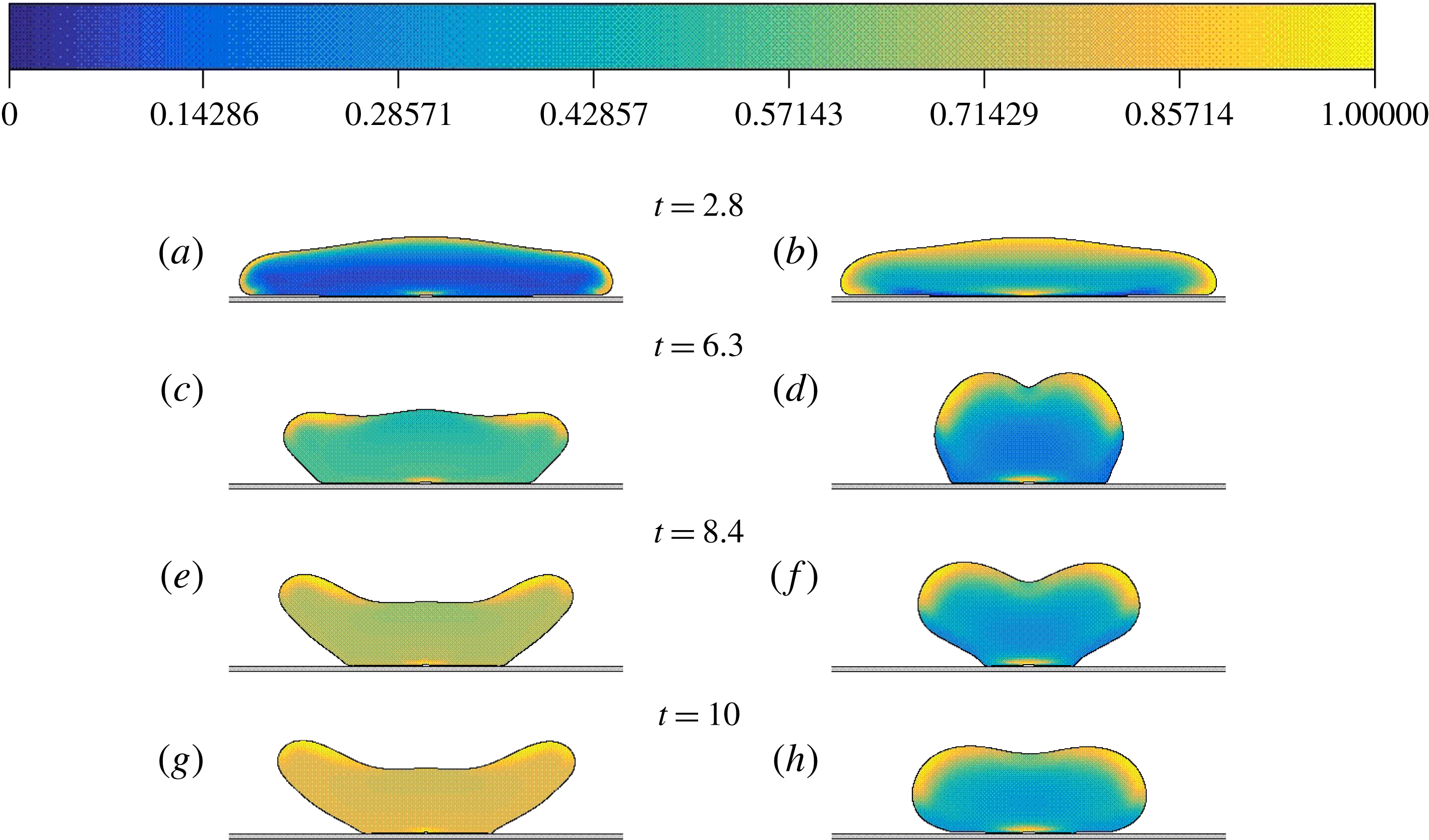
). The colour code is illustrated at the top of each of figures 12–14. Before impact, all drops present a uniform distribution of
 $\unicode[STIX]{x1D706}=1$
(fully structured state). The main purpose of showing this last set of results is to highlight the importance of thixotropy in the dynamics of the drop impact. It is interesting to note that, by keeping the dimensionless parameters
 $Re$
,
 $Wi$
,
 $\unicode[STIX]{x1D70F}_{y}$
fixed and changing the thixotropic time scale of the material, very different evolutions of the shape can happen as a consequence of the modified dynamics of the structure. In common, these figures contrast a high and a low value for the thixotropic equilibrium time,
 $t_{eq}=5$
and 20.
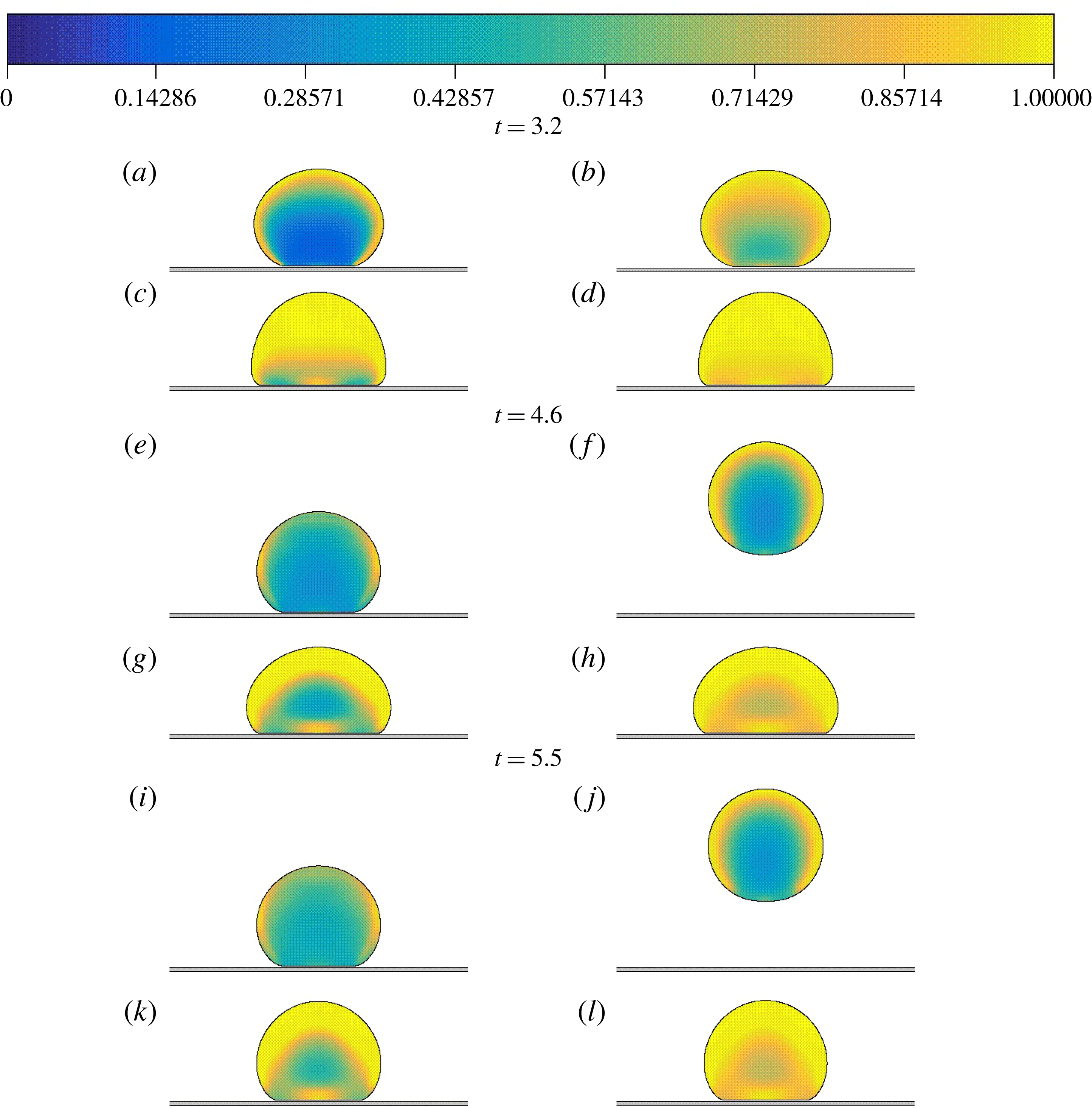
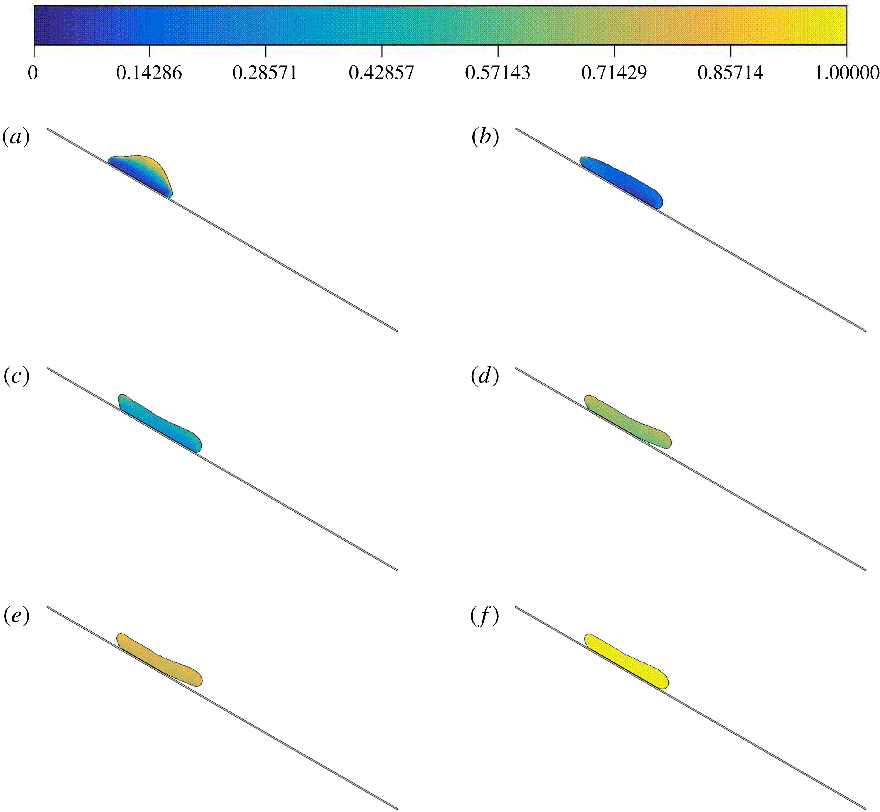
Figure 12 also shows an elastic effect by varying the Weissenberg number. The Reynolds number is low and
 $\unicode[STIX]{x1D70F}_{y}=0.7$
. At
 $t=3.2$
, just after impact, we can see that for
 $Wi=2$
(k,l), the material deforms to a higher extent than for drops with
 $Wi=0.05$
(a,b). The structural parameter of the cases in the left column, where
 $t_{eq}=5$
, are clearly lower than the cases where the thixotropic equilibrium time is higher, in the right column. This result is particularly significant in the case with low elasticity (
 $Wi=0.05-t_{eq}=5$
), since less energy is stored (compared to the case with
 $Wi=2-t_{eq}=5$
) and therefore the breakdown process is more intense. When
 $t=4.6$
, the high-
 $t_{eq}$
-low-
 $Wi$
case (b) shows a rebound. Although the Weissenberg number was low, which induced a low degree of deformation, rejuvenation was retarded by the higher value of
 $t_{eq}=20$
. Therefore, the elastic effects were still present, which enabled the drop to bounce and continue breaking down without touching the solid. Due to a very low
 $Re$
, the difference in shape that happens as a consequence of a change in
 $t_{eq}$
is not significant.
Numerical prediction of the structure parameter
 $\unicode[STIX]{x1D706}$
at different dimensionless times using
 $Re=2.05$
,
 $\unicode[STIX]{x1D70F}_{y}=0.7$
. From (column) left to right:
 $t_{eq}=5$
, 20 and from (row) top to bottom:
 $Wi=0.05$
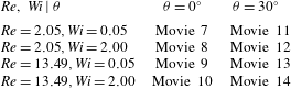
, 2. The reader will find, in the supplementary material, available at https://doi.org/10.1017/jfm.2019.541, the file Movie 1 with the video of the evolution displayed in this figure.

Numerical prediction of the structure parameter
 $\unicode[STIX]{x1D706}$
at different dimensionless times using
 $Re=13.49$
,
 $\unicode[STIX]{x1D70F}_{y}=0.7$
and
 $Wi=0.5$
. From (column) left to right:
 $t_{eq}=5,20$
. The reader will find in the supplementary material the video with the complete evolution of the motions shown in this figure.

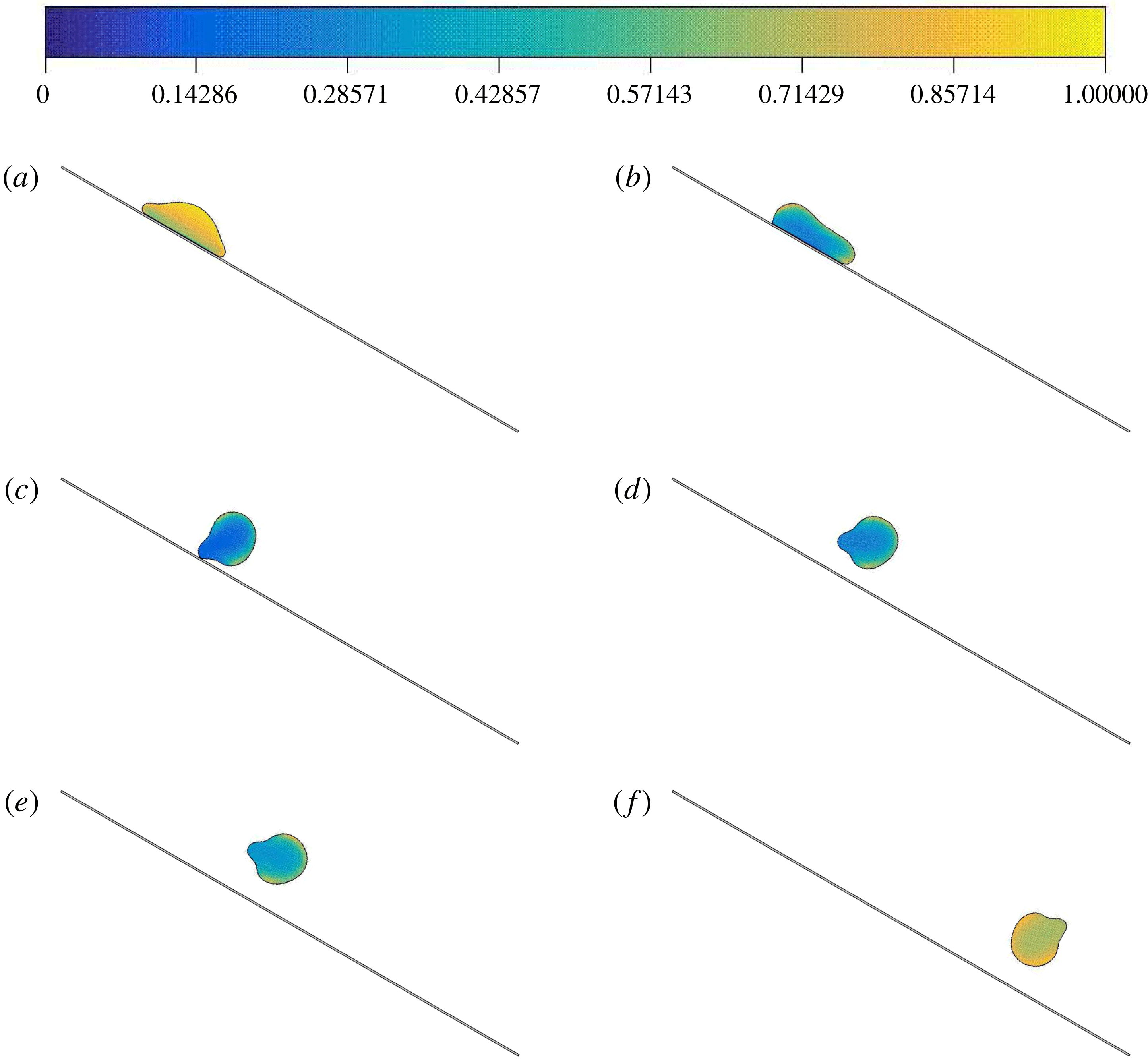
A different scenario is presented in figure 13, where the evolution of the shape is dramatically dependent on the value of
 $t_{eq}$
. In this case, a high Reynolds number was imposed. This high kinetic energy is able to produce a stress level after impact that contributes to the breakdown process. At
 $t=2.0$
, when the drops are still in the spreading stage, we can observe a reasonable difference in the distribution of the structural parameter inside the left (
 $t_{eq}=5$
) and right (
 $t_{eq}=20$
) drops. As expected, the regions of the drop which are closer to the solid surface are less structured at this instant, since they were more exposed to higher stresses. When
 $t=2.5$
, the two drops exhibit similar spreading factors, very near the maximum ones. However, we can see a small difference in shape and significant discrepancy in structure distribution, favouring more structured states in the high
 $t_{eq}$
case. The thixotropic effect on the drop configuration is particularly important in the receding stage, i.e. after the drop has reached its maximum spreading factor. Examining
 $t=4.8$
in figure 13, we can see that before this moment, the left drop has consumed the kinetic energy by breaking the material and there is not enough stored energy to provoke retraction. In this fixed configuration, the thixotropic nature of the material induces an uniform build-up process in the left drop (which continues until
 $t=10$
), since the material is exposed to an almost free stress condition. On the other hand, the right drop at
 $t=4.8$
has retracted due to elastic energy that was stored and that has been transformed into kinetic energy again. The edges of the drop initiate a motion away from the solid wall, which gradually weakens as time evolves (see
 $t=10$
).
Numerical predictions of the structural parameter
 $\unicode[STIX]{x1D706}$
at different dimensionless times using
 $Re=13.49$
,
 $\unicode[STIX]{x1D70F}_{y}=0.7$
and
 $Wi=2.0$
. Columns from left to right:
 $t_{eq}=5$
, 20. The reader will find in the supplementary material the video with the complete evolution of the motions shown in this figure.

When the Weissenberg number is increased from
 $Wi=0.5$
to 2.0, the evolutions of
 $t_{eq}$
take the form illustrated in figure 14. It is interesting to note that even when the speed of the rejuvenation process is high, such as when
 $t_{eq}=5$
(left drop), a high
 $Wi$
induces retraction after a maximum spreading obtained at
 $t\approx 6.3$
. We can see that the material remains relatively structured near the interface for this lower
 $t_{eq}$
value. Needless to say, this retraction is less intense than that for the
 $t_{eq}=20$
counterpart. Due to a rapid structure response, the analysis of
 $t=6.3$
reveals that during retraction, the left drop (which was experiencing low stress levels) initiates a build-up process. On the other hand, the higher
 $t_{eq}$
case at
 $t=6.3$
shows that the material continues to break down during retraction due to the stress inputs that were imposed before. The area of the drop that is in contact with the surface of the solid continues to decrease until
 $t=8.4$
, when the left and right drops exhibit an outward motion detaching themselves from the floor, upward in the
 $t_{eq}=5$
case and downward in the
 $t_{eq}=20$
case. From
 $t=8.4$
to 10, we can see that the high level of structure of the left drop has conferred a solid-like state that ‘freezes’ the material, while the right drop still has a liquid-like behaviour leading to a natural falling motion of the edges of the drop which were not in contact with the solid surface.
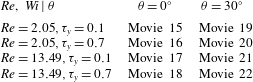
The reader will find, in the supplementary material, the file Movie 2 with the videos of the set of evolutions displayed in figures 13, 14.
5 Results: oblique drop impact
The results concerning the oblique impact of a drop on a solid surface will be presented in this section. A large variety of results were obtained as a consequence of changing the material of the drop, its impact velocity, and the inclination. We did some tests with
 $\unicode[STIX]{x1D703}=15^{\circ }$
and
 $30^{\circ }$
with respect to the horizontal plane. Since we wish to explore the influence of the inclination on the results and because we do not want to be repetitive, we focus on the case of
 $\unicode[STIX]{x1D703}=30^{\circ }$
.
5.1 Evolution of the shape and position
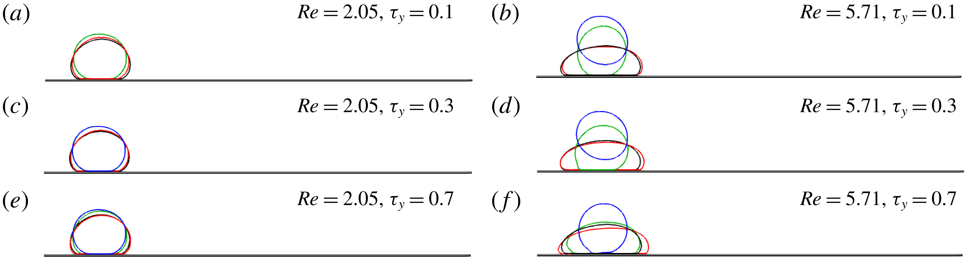
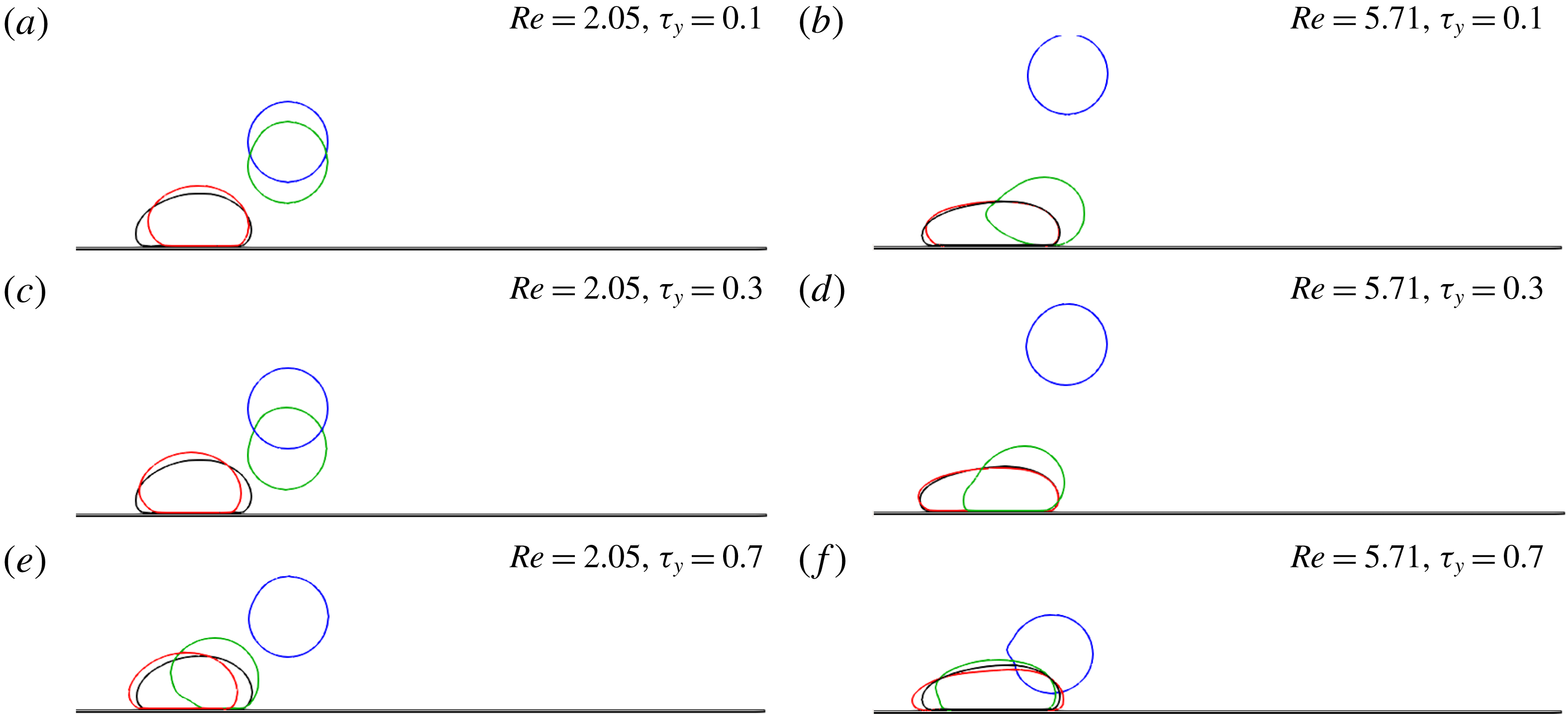
Figures 15 and 16 show two different dimensionless times,
 $t=2.5$
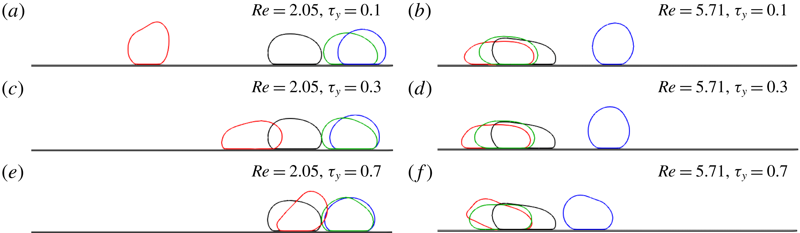
and 5.0, respectively, that correspond to the evolution of a number of cases that will be described next. In each subfigure, from (a) to (f), there are four different drops, each one corresponding to a different type of fluid, one Newtonian and three EVPT ones. The fluids are identified by the colour of their interfaces and common features of each subfigure are described in the captions of each figure. The colour code is black for the Newtonian drop, red for the drop with
 $t_{eq}=1$
, green for the drop with
 $t_{eq}=5$
and blue for the drop with
 $t_{eq}=20$
. In common, all subfigures are associated with cases of fixed Weissenberg number,
 $Wi=0.05$
. In addition to the effect of the thixotropic time, which can be analysed inside each subfigure, the comparison of the subfigures explores changes in
 $Re$
and plastic number.
Drop interface profiles for a surface at an inclination of
 $\unicode[STIX]{x1D703}=30^{\circ }$
, at dimensionless time
 $t=2.5$
. The fixed dimensionless parameter for the EVPT material is
 $Wi=0.05$
; The thixotropic times shown are
 $t_{eq}=1$
, 5, 20. The drop interface profiles considering a Newtonian fluid for different
 $Re$
are also included.

Drop interface profiles for a surface at an inclination of
 $\unicode[STIX]{x1D703}=30^{\circ }$
, at dimensionless time
 $t=5$
. The fixed dimensionless parameter for the EVPT material is
 $Wi=0.05$
; The times shown are
 $t_{eq}=1$
, 5, 20. The drop interface profiles considering a Newtonian fluid for different
 $Re$
are also included.

Drop interface profiles for a surface at an inclination of
 $\unicode[STIX]{x1D703}=30^{\circ }$
at dimensionless time
 $t=2.5$
. The fixed dimensionless parameter for the EVPT material is
 $Wi=2$
; The times shown are
 $t_{eq}=1$
, 5, 20. The drop interface profiles considering an Oldroyd-B fluid with
 $Wi=2$
for different
 $Re$
are also included.

Drop interface profiles for a surface at an inclination of
 $\unicode[STIX]{x1D703}=30^{\circ }$
at dimensionless time
 $t=18$
. The fixed dimensionless parameter for the EVPT material is
 $Wi=2$
; The times shown are
 $t_{eq}=1$
, 5, 20. The drop interface profiles considering an Oldroyd-B fluid with
 $Wi=2$
for different
 $Re$
are also included.

Taking as reference the instant
 $t=2.5$
, the left column, corresponding to subfigures 15(a), 15(c) and 15(e), have the same Reynolds number,
 $Re=2.05$
, while in the right column, corresponding to subfigures 15(b), 15(d) and 15(f),
 $Re=5.71$
. Changes in the plastic number are observed when one compares different rows. The top one, corresponding to subfigures 15(a) and 15(b), have
 $\unicode[STIX]{x1D70F}_{y}=0.1$
. In the middle row, figures 15(c) and 15(d),
 $\unicode[STIX]{x1D70F}_{y}=0.3$
; while figures 15(e) and 15(f), have their plastic numbers fixed at
 $\unicode[STIX]{x1D70F}_{y}=0.7$
. This same structure is maintained in figure 16.
At
 $t=2.5$
, just after the impact, figure 15 shows that among the cases of low Reynolds numbers, corresponding to the left column, there is no big difference between the different drops. However, for
 $Re=5.71$
, we can see a more substantial difference imposed by the particular values of
 $t_{eq}$
. While the lower value of
 $t_{eq}$
,
 $t_{eq}=1$
, exhibits a similar behaviour to the Newtonian case, higher values of
 $t_{eq}$
are associated with less deformation and, in the case of
 $t_{eq}=20$
and lower values of
 $\unicode[STIX]{x1D70F}_{y}$
, we can observe that a rebound occurs. It is important to note that the
 $t_{eq}=1$
case can be seen as a perturbation of the Newtonian case towards the EVPT material, since the dimensionless numbers that are responsible for elastic, plastic and thixotropic effects are low (
 $Wi=0.05$
,
 $\unicode[STIX]{x1D70F}_{y}=0.1$
,
 $t_{eq}=1$
). When the time is advanced to
 $t=5.0$
, we can see from the analysis of figure 16 that the blue drop corresponding to
 $t_{eq}=20$
bounces even when
 $Re=2.05$
, and the position and shape of the red drop (
 $t_{eq}=1$
) still gravitate around those of the Newtonian drop.
Another set of evolutions is depicted in figures 17 and 18, corresponding to
 $t=2.5$
and 18, respectively. Again, the left and right columns are identified with
 $Re=2.05$
and 5.71, respectively, and the top, middle and bottom rows are identified with
 $\unicode[STIX]{x1D70F}_{y}=0.1$
,
 $\unicode[STIX]{x1D70F}_{y}=0.3$
and
 $\unicode[STIX]{x1D70F}_{y}=0.7$
, respectively. The difference between this and the previous set is the Weissenberg number, which in the present set is
 $Wi=2$
. Another important change is that for comparison with the EVPT drops we chose as reference an Oldroyd-B viscoelastic fluid (with the same
 $Wi=2$
). In figure 17, which corresponds to
 $t=2.5$
, we can see immediately that after this oblique impact, these drops deform more than the ones with low
 $Wi$
shown in figure 15. Again, we can see that in the right column the drops exhibit more spreading than in the left column, where the kinetic energy transferred to the drop is lower.
Inclination angle of
 $15^{\circ }$
.

During the evolution until
 $t=18$
, rolling (with its variant, sliding) is the main result of this set of numerical experiments. The plastic and purely viscous deformations in the retraction process have consumed the elastic energy and no bouncing is to be seen. After retraction, some shapes achieve a stable configuration in that the stresses caused by gravity and the contact with the solid, together with the dynamics of aging and rejuvenation, find an equilibrium. The black drop (Oldroyd-B fluid) is not influenced by the plastic number, and therefore its shape and position do not change from one row to another. In this connection, we can see that the viscoplastic-thixotropic effects that change the viscous and elastic properties of the EVPT drops also change the dynamics of their evolution in a complex manner that makes their behaviour deviate from a purely elastic behaviour.
The reader will find, in the supplementary material, the files Movie 3 and Movie 4 with the videos of the set of evolutions displayed in this subsection.
5.2 Main outputs of the oblique drop impact
The complexity introduced by the oblique impact was not able to be captured by the quantities,
 $Oh_{e}$
and
 $Y$
, that were used in the normal drop impact. An additional qualitative output was included: rolling. We found non-monotonic trends associated with the original dimensionless numbers, as shown in figures 19 and 20 for inclination angles of
 $15^{\circ }$
and
 $30^{\circ }$
, respectively. However, the use of
 $Y$
and
 $Oh_{e}$
could separate tendencies. We can say that, for low
 $Y$
values and low
 $Oh_{e}$
there is tendency to have a bouncing output. The rolling output is achieved for low
 $Y$
and high
 $Oh_{e}$
. The same critical elastic Ohnesorge number,
 $Oh_{ec}=0.5$
, confines bouncing results for both inclination angles. High
 $Y$
values lead to the drop to stick. For the highest thixotropic equilibrium time tested,
 $t_{eq}=20$
, we had bouncing and rolling results only. In addition, we found no dependence on the inclination angle for the outputs in this high
 $t_{eq}$
regime. Using
 $M/\unicode[STIX]{x1D6FE}_{y}$
, as in Luu & Forterre (Reference Luu and Forterre2009), to compose with
 $Oh_{e}$
the two-dimensional Cartesian space we were able to separate bouncing from rolling, as figure 21 reveals. It is not a coincidence that the same critical value for
 $Oh_{e}$
is found. Among the chosen
 $t_{eq}$
values, only in the inclined cases with the highest thixotropic equilibrium time, the results were clearly separated into two regions and a critical
 $Oh_{e}$
could be found; for
 $Oh_{ec}>0.5$
no bouncing occurred. The graphs corresponding to the inclination angles of
 $15^{\circ }$
and
 $30^{\circ }$
are shown in figure 21. In fact, for
 $t_{eq}=20$
there was no difference between the two tested inclination values.
Inclination angle of
 $30^{\circ }$
.

Inclination angle of
 $15^{\circ }$
or
 $30^{\circ }$
for
 $t_{eq}=20$
.

Numerical prediction of the structural parameter
 $\unicode[STIX]{x1D706}$
at different dimensionless times using
 $Re=13.49$
,
 $\unicode[STIX]{x1D70F}_{y}=0.7$
,
 $t_{eq}=5$
and
 $Wi=0.5$
for a surface at an inclination of
 $\unicode[STIX]{x1D703}=30^{\circ }$
. The reader will find, in the supplementary material, the file Movie 5 with the video of the complete evolution of the case shown in this figure.

In appendix B we show the general outputs (stick, rolling and bouncing) according to the combinations of the values of the four dimensionless numbers explored in the present paper.
5.3 Evolution of the shape, position and structure for an oblique drop impact
Figures 22, and 23 show successive changes in time of the structural parameter field, together with the shape and position as the drop evolves after an oblique collision, with a high impact velocity (
 $Re=13.49$
). In this set of figures, the plane is exhibited with an inclination of
 $\unicode[STIX]{x1D703}=30^{\circ }$
and gravity acts in the vertical direction.
In figure 22, the drop exhibits a kind of ‘mushroom head’ shape just after impact, figure 22(a), where we can clearly see a much more intense rejuvenation in the regions near the wall because of the low value of
 $t_{eq}$
, which induces rapid destruction. Since
 $Re$
is high, the drop evolves in the subsequent frame, figure 22(b), to a very stretched configuration with a very low degree of structure, quite uniformly distributed. In this configuration, the gravitational forces are not strong enough to induce more breaking and to overcome the overall viscous resistance: so, the drop almost does not change position, presenting slight changes in shape. At this stage, the build-up process begins and structuring takes place in the evolving drops.
Figure 23 shows a case where rebound occurs in the oblique impact problem. In this case, a reasonable deformation occurs during the spreading stage after impact, and the retraction process takes place with a high level of stored energy, enabling the drop to be expelled from the surface of the solid. In other words, this rebound is not a direct effect of the deformation associated with the direction normal to the inclined plane, but with a deformation, extension and retraction in the direction of the inclined plane. The instant after impact, shown in subfigure figure 23(a), has the same ‘mushroom-head’ shape, where the bottom region has less structure due to the breakdown process that occurs as a result of the impact. The next frame, figure 23(b), shows a ‘black bean’ shape, where a more severe breakdown has happened and the drop is still retracting. This retraction continues from both sides and induces an out-of-the-plane motion and in figure 23(c) the drop has just left the solid, leaving a nub near the point of its last contact. After leaving the plane, the drop does not change its shape significantly, developing a rotating trajectory and an aging process.
Numerical prediction of the structural parameter
 $\unicode[STIX]{x1D706}$
at different dimensionless times using
 $Re=13.49$
,
 $\unicode[STIX]{x1D70F}_{y}=0.3$
,
 $t_{eq}=20$
and
 $Wi=0.5$
for a surface at an inclination of
 $\unicode[STIX]{x1D703}=30^{\circ }$
. The reader will find, in the supplementary material, the file Movie 6 with the video of the complete evolution of the case shown in this figure.

6 Concluding remarks
The present paper has investigated the drop impact of yield stress fluids onto a solid flat surface. Although this kind of fluid has, as a fingerprint, the presence of a yield stress as a mechanical property, a purely viscoplastic model is not able to reproduce the experimental results. So it is of crucial importance that the modelling include other features, such as elasticity and thixotropy, in order to yield more realistic results. Another important remark is that the presence of a yield stress generally inhibits capillary effects, which can be neglected in a number of applications, and this was done in the present study. We explored combinations of the Reynolds number, Weissenberg number, plastic number and dimensionless thixotropic equilibrium time, dimensionless numbers that aim to capture inertial, elastic, plastic and thixotropic effects, respectively, in each of these two problems, normal and oblique drop impact.
The examination of the evolution of the height and the diameter of the drop in normal impact corroborated important experimental findings in the literature, one of which is that the spreading stage has a marked dependence on the impact velocity and only a weak dependence on the mechanical properties of the fluid drop, while what happens after the diameter achieves its maximum value depends significantly on the rheology of the fluid (Bertola Reference Bertola2012). Another documented experimental aspect that was corroborated in the present paper is that the rebound, as well as oscillations in the diameter after reaching the point of maximum spreading, attributed to the stored interfacial energy in the Newtonian drop impact problem, do appear in complex fluids that present elastic properties when interfacial forces are neglected (Luu & Forterre Reference Luu and Forterre2009). In this regard, we found a critical value for the elastic Ohnesorge number (the corresponding
 $Oh$
for drops with elasticity) above which no bouncing takes place. Thixotropic effects become more important when the impact velocity is increased. When the fluid is more thixotropic, the probability of bouncing is higher. In addition, when the drop remains attached to the solid surface, the drops which are more thixotropic tend to oscillate around smaller diameters (closer to the original drop diameter) than do the less thixotropic drops, which oscillate around greater diameters (closer to the maximum spreading factor configuration). For drops with lower elasticity, the diameter does not oscillate significantly after spreading and the thixotropic effect is found on the maximum diameter achieved, since the delay in destruction leads to more retraction. The plastic number also influences this final configuration: high values of
 $\unicode[STIX]{x1D70F}_{y}$
favour the drop’s maintaining a larger diameter, as the yield stress inhibits the drop from being destroyed. An increase of elastic effects, as captured by
 $Wi$
, leads to a smaller number of rebounds, showing that the mechanical property associated with elasticity can lead to bounce inhibition. The problem gains additional interest when the evolution of the shape and structure are examined with more attention. The shapes can assume rather complex forms during evolution and the structural level of the fluid reveals the distribution of more liquid-like and more solid-like states inside the drop domain.
The impact on an inclined solid surface exhibited a rich variety of results, as already reported in the limited experimental literature for Newtonian-capillary problems. As in the case of the normal drop impact, we can see that the elastic energy stored in the material induces results that are similar to those found in experiments with Newtonian drops with non-negligible interfacial tension. Not only the evolution of the shape, but also the evolution of the position of the drops in the inclined plane of the solid surface can be very different, depending on the rheology, due to rolling. The drops can roll with more or less deformation, which in turn has an effect on the shape during its trajectory. Rolling can occur, maintaining the drop’s shape in two different ways. The drop can roll, rotating around a centre point located inside the drop, giving the impression of an apparent sliding motion. Another kind of rolling with fixed shape is when the rotation is about a point of contact with the solid surface.
Normal and oblique impacts can exhibit rebounds that can be classified into two kinds. One occurs when the deformation is small, due to the rigidity of the drop. Just after impact, the solid induces bouncing and the drop leaves the surface before receding. The other happens after a more extended deformation. Then, the retraction has enough energy to expel the drop from contact with the solid (Antonini et al. Reference Antonini, Jung, Wetzel, Heer, Schoch, Moqaddam, Chikatamarla, Karlin, Marengo and Poulikakos2016).
In summary, the present work shows that thixotropic effects can be significantly important in the drop impact problem of yield stress fluids. Although rare in the literature, a model that accounts for thixotropy can provide more reliable results.
For further steps, we think it would be important to investigate the role played by surface tension forces and other wetting features in the drop impact on solid surfaces. In addition, it would be a significant step to address how elasto-viscoplastic thixotropic fluids behave in related problems such as the drop impact on substrates with a thin film of liquid, as well as the entry flow on a liquid in a deep reservoir.
Set of evolutions with plastic number and dimensionless thixotropic time fixed. In the left column,
 $\unicode[STIX]{x1D70F}_{y}=0.1$
and
 $t_{eq}=5$
. In the right column,
 $\unicode[STIX]{x1D70F}_{y}=0.7$
and
 $t_{eq}=20$
.

Set of evolutions with Weissenberg and dimensionless thixotropic time fixed. In the top left position,
 $Wi=0.05$
and
 $t_{eq}=5$
. In the top right position,
 $Wi=0.05$
and
 $t_{eq}=20$
. In the bottom left position,
 $Wi=2.00$
and
 $t_{eq}=5$
. In the top right position,
 $Wi=2.00$
and
 $t_{eq}=20$
.

Acknowledgements
C.M.O. acknowledges the financial support of FAPESP (Fundação de Amparo à Pesquisa do Estado de São Paulo) Grant 2013/07375-0 and CNPq (Conselho Nacional de Desenvolvimento Cientifico e Tecnologico), Grant 307459/2016-0. R.L.T. acknowledges the financial support of CNPq (Conselho Nacional de Desenvolvimento Cientifico e Tecnologico), Grant 309004/2014-4.
Temporal evolution of the normalized drop diameter
 $D(t)/D_{0}$
for Case 1 (a) and minimum bounce height
 $H(t)/D_{0}$
(b) for Case 2 using three meshes.

Free-surface profiles at selected dimensionless times (
 $t(U_{i}/D_{0})=3,5,7$
) on meshes M1, M2 and M3 (
 $\text{sol}_{ref}$
) for Case 1 and Case 2.

Map of the type of impact as a function of the dimensionless parameters
 $Re$
,
 $Wi$
,
 $\unicode[STIX]{x1D70F}_{y}$
and
 $t_{eq}$
. Empty circles indicate impacts without rebounding nor rolling, fully filled circles indicate cases with rebounding, and semi-filled circles indicate rolling. From top to bottom, inclination angles of
 $0^{\circ }$
,
 $15^{\circ }$
, and
 $30^{\circ }$
.

Supplementary movies
Supplementary movies are available at https://doi.org/10.1017/jfm.2019.541. In addition to the files: Movie 1, Movie 2, Movie 3, Movie 4, Movie 5, Movie 6, which contain videos that correspond to figures shown in the present work, the reader will find, in the supplementary material, other videos with new sets of evolutions that can be illustrative examples of normal and oblique drop impact behaviour of complex fluids. Tables 1 and 2 show the dimensionless parameters and the names of the corresponding videos.
Appendix A. Mesh refinement study
In order to validate the numerical strategy for solving this complex flow, we have used a mesh refinement study considering three uniform meshes. On the coarse mesh, denoted here by M1, 40 cells are considered per drop diameter, whereas for the intermediate (M2) mesh, 80 cells are used. The finest mesh, M3, is employed here as a reference solution (
 $\text{sol}_{ref}$
): it has a grid resolution of 160 cells per drop diameter. Two different cases, referred to as Case 1 and Case 2, have been investigated, considering different dimensionless parameters, as can be viewed in table 3. In these simulations, the fixed parameters are
 $\unicode[STIX]{x1D70F}_{y}=0.1$
and
 $t_{eq}=5$
. These two cases were carefully selected in order to show the numerical convergence for two different results of the problem: non-bouncing and bouncing.
In order to investigate the influence of the grid resolution on the numerical convergence in the non-bouncing case, we will compare the spreading diameter
 $D(t)/D_{0}$
(see figure 2
a) as a function of time for M1, M2 and M3 (
 $\text{sol}_{ref}$
). In figure 24(a), we can see the numerical convergence of the solutions for Case 1.
In terms of the bouncing dynamics, the mesh refinement study is conducted to measure the time variation of the minimum bounce height
 $H(t)/D_{0}$
, while varying the three meshes, as presented in figure 24(b). In particular, the minimum drop height has been calculated considering the vertical distance between the solid wall and the lowest point located at the bottom interface with the drop, as illustrated in figure 2(b). In figure 24(b) it is possible to see the good agreement between the result provided using mesh M2 and the reference solution.
Dimensionless parameters used to verify the proposed methodology.

We have also investigated the free surface shape of the drops for the two cases at different times. The results for the non-bouncing case are given in figure 25(a) while figure 25(b) gives the results for the bouncing case. From these figures, we can confirm the adequate convergence of the free surface with a mesh refinement.
Therefore, the results for Case 1 and Case 2 for M2 and M3 (
 $\text{sol}_{ref}$
) are very similar, and thus the M2 mesh has been adopted for the all simulations in the present work.
Appendix B. Maps of results
Figure 26 show the maps of the main outputs of these processes where we can see a quick overview of the influence of the four dimensionless numbers.