

Introduction
Because graphene is two-dimensional,Reference Geim1, Reference Novoselov, Geim, Morozov, Jiang, Zhang, Dubonos, Grigorieva and Firsov2 scanning tunneling microscopy (STM) is ideal for its characterization.Reference Güntherodt and Wiesendanger3, Reference Binning, Rohrer, Gerber and Weibel4 To date, many STM studies have been carried out on graphene.Reference Brar, Zhang, Yayon, Ohta, McChesney, Bostwick, Rotenberg, Horn and Crommie5–Reference Wong, Huang, Wang, Cao, Qi, Santoso, Chen and Wee9 Because of its atomic resolution, STM is able to probe important local physical and electronic details of both pristine and modified epitaxial graphene that other techniques are unable to access. In this review, we first introduce the basic working principles and setups used for STM and scanning tunneling spectroscopy (STS).The capabilities of STM/STS are then illustrated by instructive examples of epitaxial graphene characterization. Molecular interactions, intercalation, and fundamental studies of epitaxial graphene are also discussed.
Principles of STM
When an atomically sharp STM tip is brought within a few nanometers of a surface and a voltage bias (from a few millielectronvolts to a few electronvolts) is applied across the gap, electrons can quantum-mechanically tunnel through the potential barrier presented by the gap. This induced tunneling current is exponentially dependent on the gap distance, enabling STM to be a highly sensitive probe. Spatial variation in surface topography can thus be detected through changes in tunneling current. The electronic charge density distribution on the surface also determines the location and energy from which electrons tunnel, thereby allowing imaging of the precise atomic and electronic structure of the surface.
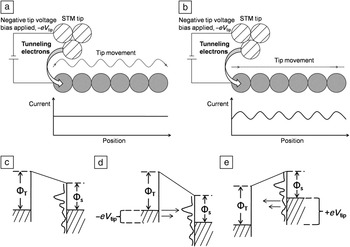
Tip motion is controlled by a piezoelectric mount that responds mechanically to small changes in the applied voltage. There are two modes of topographical imaging: The first is constant-current mode, in which the tunneling current is kept constant by means of a feedback loop as the tip scans across the surface. This current feedback loop instructs the tip to retract from (approach) the surface when there is an increase (decrease) in the current. The other mode is constant-height mode, in which the current is allowed to vary as the tip is scanned across the surface at a fixed distance above it. Schematics for constant-current and constant-height modes are shown in Figure 1a–b, respectively.
(a–b) Schematics of a scanning tunneling microscope in (a) constant-current and (b) constant-height modes. (c–e) Energy level diagrams for the sample and tip, where Φs and ΦT represent the corresponding work functions. Dashed lines, vacuum levels; solid horizontal lines, Fermi levels below which sample states are occupied; wavy lines, sample density of states (DOS). (c) Sample and tip at thermal equilibrium, separated by a small vacuum gap, with zero applied voltage bias and thus no electron flow. (d) Same as (c) but with negative tip bias, so that electrons tunnel from the occupied electronic states of the tip to the unoccupied states of the sample. (e) Same as (d) but with positive tip bias, so that electrons tunnel in the opposite direction. Parts (c)–(e) adapted from Reference Reference Hamers10.

The resultant variation of the tip height or current with the tip position is recorded as an STM topography image. STM can be performed in a liquid or at pressures ranging from atmospheric pressure to ultrahigh-vacuum (UHV) conditions of less than 10–9mbar. In this review, we focus on STM in UHV, where the ultimate atomic resolution is routinely achievable because contamination is minimized.
The current that an STM tip emits or receives due to quantum-mechanical tunneling is a combination of three factors: applied voltage, distance between tip and surface, and local density of electronic states (DOS). The voltage determines the difference in the Fermi energy level between the tip and surface and, thus, the number of tunneling electrons. The probability of electron tunneling between the tip and surface decreases exponentially with the distance between them. The DOS at specific energies of both the tip and surface determines how many electrons can tunnel. These factors are illustrated in the energy level diagrams of Figure 1c–e.Reference Hamers10
Techniques such as photoemission spectroscopy measure the average DOS over an area, but STM measures the variation of the local DOS at the atomic scale. STS probes the energy dependence of the local electronic structure and the effects that surface impurities have on it.
During STS, the tip–sample distance is kept constant by turning off the constant-current feedback loop. A voltage bias applied across the tip and sample is varied, and the measured derivative of the current with respect to the applied voltage, the differential tunneling conductance (dI/dV), is recorded. A negative tip bias V tip (equivalent to a positive sample bias, V sample, of the same magnitude) probes the DOS of the sample above the Fermi level. A positive V tip (or negative V sample) probes states below the Fermi level. The DOS is directly proportional to dI/dV.
For greater signal-to-noise ratio, an electronic lock-in method is used whereby a high-frequency sinusoidal voltage modulation is superimposed on the applied voltage bias. The first harmonic of the modulated current then gives the desired differential conductance. In particular, for dI/dV mapping, the voltage bias is kept constant, and the derivative of the current is recorded as the tip scans. Hence, the spatial distribution of electronic states with energy specified by the applied voltage bias can be probed.
Physical characterization
The appearance of graphene under a scanning tunneling microscope varies with the applied bias, as well as the number of layers. At higher voltage biases, the graphene atomic structure of epitaxially grown graphene is not easily imaged because there are energetically accessible electronic states in both the graphene and underlying substrate. This is shown in Figure 2 for graphene on the silicon-terminated basal plane of SiC, otherwise known as the Si face or SiC(0001) (see the article in this issue by Nyakiti et al.). At a tip voltage bias of 1.78 V, the underlying buffer layer is observed in Figure 2a instead of the atomic-scale honeycomb structures of graphene.Reference Huang, Chen, Chen and Wee11
(a) Typical scanning tunneling microscopy (STM) image (100 × 100 nm2, V tip = 1.78 V) of monolayer and bilayer epitaxial graphene (EG) on 6H-SiC(0001), with the line profile across the monolayer and bilayer regions superimposed in white. (b) High-resolution STM image (20 × 20 nm2, V tip = 0.5 V) of a typical boundary, from the boxed region in panel (a), showing the coexistence of monolayer and bilayer EG, with corresponding atomically resolved STM images (1.5 × 1.5 nm2, V tip = –0.1 V) in the insets. (c) Corresponding detailed image (8 × 8 nm2, V tip = –0.1 V), clearly revealing the physical continuum at the domain boundaries between monolayer and bilayer EG. The inset shows the Bernal stacking of bilayer graphene. (d) Schematic model of the atomic structures of neighboring monolayer and bilayer EG on the same terrace. Blue bars represent the buffer layer on Si-face SiC, which has a  $6\sqrt 3 \times 6\sqrt 3 R30^\circ $ reconstruction. Reproduced with permission from Reference Reference Huang, Chen, Chen and Wee11. ©2008, American Chemical Society.

At low biases (<0.4 V), however, electron tunneling from graphene dominates because of a lack of SiC electronic states in the bandgap of the substrate. The graphene electronic orbitals involved are the low-lying π orbitals, which reflect the six-membered benzene rings of graphene. These rings are visible in the monolayer regions of the high-resolution STM images of Figure 2b–c. For bilayer graphene, three-fold symmetry is observed because the AB (Bernal) layer stacking distinguishes the two carbon atoms in the graphene unit cell (colored blue and red in the top inset of Figure 2b).
As described earlier, the interfacial buffer layer can be imaged under the graphene and contributes to the surface roughness measured by STM.Reference Mallet, Varchon, Naud, Magaud, Berger and Veuillen12–Reference Emtsev, Speck, Seyller and Ley19 This roughness decreases with the number of graphene layers, as shown in the line profile in Figure 2a.Reference Huang, Chen, Chen and Wee11 The roughness of the imaged underlying buffer layer is larger over the monolayer graphene in the center than over the bilayer graphene at the sides, allowing one to distinguish between regions with different numbers of graphene layers.
The growth modes of epitaxial graphene on metalReference N’Diaye, Engler, Busse, Wall, Buckanie, Meyer zu Heringdorf, van Gastel, Poelsema and Michely20–Reference Lahiri, Miller, Adamska, Oleynik and Batzill24 or SiCReference Huang, Chen, Chen and Wee11–Reference Veuillen, Hiebel, Magaud, Mallet and Varchon13, Reference Lahiri, Miller, Adamska, Oleynik and Batzill24–Reference Hupalo, Conrad and Tringides31 substrates can also be investigated by STM. An example is epitaxial graphene on SiC(0001). Regions of monolayer graphene are seen to be continuous with those of bilayer graphene in Figure 2c. Step heights of 0.09 nm, 0.34 nm, and 0.25 nm are also measured across various steps. These heights cannot be solely attributed to the variations in the substrate terraces, as each SiC bilayer is 0.25 nm in height.
The arrangement of the epitaxial graphene layers and the associated height variation is modeled in Figure 2d. This model, in which the number of layers changes immediately at a substrate step, directly reflects an assumed reverse step-flow growth mechanism. Growth occurs with sublimation of silicon atoms from three SiC bilayers to form a new buffer layer, and the silicon–carbon bonds of the pre-existing buffer layer break to form a new graphene layer. By depositing cobalt atoms, which form physisorbed clusters of high (low) density on the buffer layer (graphene) surface and observing the height changes with annealing temperature and time, Poon et al. confirmed the same phenomena.Reference Poon, Chen, Tok and Wee28, Reference Poon, Chen, Wee and Tok29
Rotational mismatch between graphene layers can also be determined by STM. For silicon-terminated SiC, because of the bottom-up growth mode and the presence of an interfacial buffer layer with well-defined orientation, all of the grown graphene layers are Bernal stacked. However, on carbon-terminated SiC(000 $\bar 1$), adjacent graphene layers have random orientations because of the absence of a similar buffer layer.Reference First, de Heer, Seyller, Berger, Stroscio and Moon27 The graphene layers are rotationally disordered and effectively decoupled, both physically and electronically.Reference First, de Heer, Seyller, Berger, Stroscio and Moon27, Reference Sprinkle, Siegel, Hu, Hicks, Tejeda, Taleb-Ibrahimi, Le Fèvre, Bertran, Vizzini, Enriquez, Chiang, Soukiassian, Berger, de Heer, Lanzara and Conrad32–Reference Hass, de Heer and Conrad34 This is demonstrated in Figure 3, where rotational disorder is present between the top two layers of multilayer graphene grown on SiC(000
 $\bar 1$).Reference Hass, de Heer and Conrad34, Reference Hass, Varchon, Millán-Otoya, Sprinkle, Sharma, de Heer, Berger, First, Magaud and Conrad35 Because of the ~30° rotation between these two layers, a
 $\sqrt {13} \times \sqrt {13} R46.1^\circ $ superlattice is observed in Figure 3a. Such disorder results in the graphene layers not being Bernal stacked, in contrast to those of graphite and epitaxial graphene grown on the Si face of SiC(0001). In Figure 3b, one can still faintly make out the hexagonal structure, with three of the six atoms having a lower intensity because of the presence of a misaligned bottom layer. The small size of this effect indicates effective decoupling between the layers. Indeed, magnetotransport and STS measurements of such systems yield signature monolayer graphene results.Reference First, de Heer, Seyller, Berger, Stroscio and Moon27, Reference Song, Otte, Kuk, Hu, Torrance, First, de Heer, Min, Adam, Stiles, MacDonald and Stroscio36–Reference Miller, Kubista, Rutter, Ruan, de Heer, First and Stroscio38
Rotational stacking faults between layers in multilayer epitaxial graphene (MEG) on SiC(000 $\bar 1$). (a) STM topograph showing the moiré superlattice on the top layer of a nominally 10-layer MEG sample. (b) High-resolution image of the
 $\sqrt {13} \times \sqrt {13} R46.1^\circ $ superlattice. (c)
 $\sqrt {13} \times \sqrt {13} R46.1^\circ $ unit cell of the moiré pattern with respect to the topmost graphene layer. a and b are graphene unit vectors. Dark circles are carbon atoms; gray circles are carbon atoms of the layer below, rotated by 32.204° from the top layer. Reproduced with permission from Reference Reference Hass, Varchon, Millán-Otoya, Sprinkle, Sharma, de Heer, Berger, First, Magaud and Conrad35. ©2008, American Physical Society.

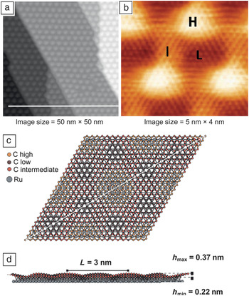
For growth on metals, the incommensurability of lattice constants between the graphene layer and the underlying substrate produces moiré patterns that can be observed by STM.Reference Cho, Gao, Tian, Cao, Wu, Yu, Yitamben, Fisher, Guest, Chen and Guisinger8, Reference N’Diaye, Engler, Busse, Wall, Buckanie, Meyer zu Heringdorf, van Gastel, Poelsema and Michely20, Reference Gao, Guest and Guisinger39–Reference Jin, Fu, Mu, Tan and Bao46 Because of the in-plane lattice mismatch between graphene (2.41 Å) and Ru(0001) (2.71 Å), for example, the positions of carbon atoms relative to metal atoms vary with a periodicity of 30 Å. This periodicity manifests as a moiré pattern,Reference Huang, Pan, Pan, Gao, Xu, Que, Zhou, Wang, Du and Gao44–Reference Pan, Zhang, Shi, Sun, Du, Liu and Gao47 as shown in Figure 4a.Reference Marchini, Günther and Wintterlin48
(a–b) STM images of a Ru(0001) surface with adsorbed graphene, prepared by segregation of carbon from the bulk. (a) Fully covered surface after annealing at 1470 K, showing the hexagonal Ru(0001)/graphene moiré pattern, which is much larger than the graphene unit cell. (b) Atomically resolved STM image of the moiré pattern in (a), also revealing the graphene periodicity. The high (H), intermediate (I), and low (L) regions correspond to different alignments between the graphene and the metal substrate. Parts (a) and (b) reproduced with permission from Reference Reference Marchini, Günther and Wintterlin48. ©2007, American Physical Society. (c) Top and (d) side views of four unit cells of the moiré structure, 6 nm × 5.2 nm. For clarity, only one layer of ruthenium atoms is shown in (c). The diagonal line cuts across the I and H regions. In (d), the buckling of the graphene layer can be clearly seen, where h min and h max are the minimum and maximum heights, respectively, of the graphene above the metal surface. Parts (c) and (d) reproduced with permission from Reference Reference Wang, Bocquet, Marchini, Günther and Wintterlin49. ©2008, Royal Society of Chemistry.

Figure 4b reveals that the moiré pattern has three regions of different contrast: low (L), intermediate (I), and high (H) areas.Reference Wang, Bocquet, Marchini, Günther and Wintterlin49 In the high region, both carbon atoms occupy hollow sites, residing on alternating fcc/hcp sites and forming no bond with the substrate. In the intermediate areas, the carbon atoms are situated near bridge sites of the metallic substrate and are imaged as linear stripes of protrusions. For low regions, where the apparent height is the lowest, one carbon atom sits on an atop site, and the other is above either an fcc or hcp site. Because the carbon atoms are situated directly above the ruthenium atoms, carbon–ruthenium chemical bonds are formed, and the DOS of the carbon atoms at the Fermi level is reduced. Only the atoms that are not bonded are visible by STM. Thus, all six atoms are observed in the high regions, and only three of the six atoms are observed in the low regions. The bright/dark contrast is inverted in the low regions because of the periodic reversal in the position of the second carbon atom from fcp to hcp positions on the substrate.
Electronic characterization
STS can detect changes in the electronic structure of graphene, such as quantization of electronic states in a magnetic fieldReference Song, Otte, Kuk, Hu, Torrance, First, de Heer, Min, Adam, Stiles, MacDonald and Stroscio36, Reference Miller, Kubista, Rutter, Ruan, de Heer, Kindermann, First and Stroscio50, Reference Jung, Rutter, Klimov, Newell, Calizo, Hight-Walker, Zhitenev and Stroscio51 or electronic perturbations due to interlayer effects,Reference Li, Luican, Lopes dos Santos, Castro Neto, Reina, Kong and Andrei52, Reference Li, Luican and Andrei53 deformation,Reference Levy, Burke, Meaker, Panlasigui, Zettl, Guinea, Neto and Crommie54, Reference Yan, Sun, He, Nie and Chan55 and physical confinement.Reference Subramaniam, Libisch, Li, Pauly, Geringer, Reiter, Mashoff, Liebmann, Burgdörfer, Busse, Michely, Mazzarello, Pratzer and Morgenstern56, Reference Tapaszto, Dobrik, Lambin and Biro57 These measurements also reveal dramatic differences between monolayer and bilayer graphene.
Dispersion relations
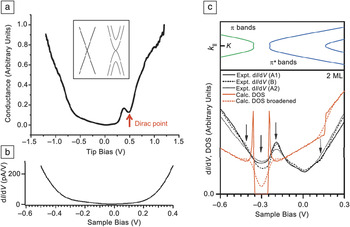
Graphene monolayers and bilayers exhibit linear and parabolic band dispersions, respectively (inset of Figure 5a).Reference Castro Neto, Peres, Novoselov and Geim58, Reference Wallace59 For monolayer graphene, the DOS is linearly proportional to the crystal momentum near the Dirac point and is zero at the Dirac point. This is reflected in scanning tunneling (ST) spectra as a dip in the conductance. Bandgaps can also be identified by the absence of conductance.
(a) Scanning tunneling (ST) spectrum, showing the conductance, dI/dV, as a function of tip bias, V tip, for a pristine monolayer on SiC(0001). Inset shows the schematic band structures of pristine monolayer (left) and bilayer (right) graphene, which exhibit linear and parabolic dispersions, respectively. Part (a) reproduced with permission from Reference Reference Wong, Huang, Wang, Cao, Qi, Santoso, Chen and Wee9. ©2011, American Chemical Society. (b) ST spectrum versus V sample = –V tip of graphene covalently bonded to aryl radicals, showing a featureless bandgap straddling the Fermi level (V sample = 0 V). Part (b) reproduced with permission from Reference Reference Hossain, Walsh and Hersam60. ©2010, American Chemical Society. (c) Top: Band structure of pristine bilayer graphene on SiC(0001). Bottom: Theoretical and experimental ST spectra versus V sample for pristine bilayer graphene on SiC(0001). The arrows indicate the associated increase in DOS at the conduction-band maxima and valence-band minima at sample biases of –0.5 V and –0.2 V, respectively, and that of the Dirac point at a sample bias of –0.3 V. The arrow at a sample bias of +0.15 V indicates the inflection of the DOS due to the theoretically predicated steplike increase in DOS. A1, A2, and B represent different locations on the sample. Part (c) reproduced with permission from Reference Reference Lauffer, Emtsev, Graupner, Seyller and Ley7. ©2008, American Physical Society.

A characteristic ST spectrum obtained from monolayer graphene on SiC(0001) is shown in Figure 5a.Reference Wong, Huang, Wang, Cao, Qi, Santoso, Chen and Wee9 The minimum at zero bias is characteristic of two-dimensional electronic systems. The other minimum located 0.4 eV below the Fermi level (occupied states, positive tip bias) reflects the position of the Dirac point. This implies electron doping of graphene due to charge transfer from the interfacial layer.Reference Bostwick, Emtsev, Horn, Huwald, Ley, McChesney, Ohta, Riley, Rotenberg, Speck and Seyller16, Reference Emtsev, Speck, Seyller and Ley19
In another example, Figure 5bReference Hossain, Walsh and Hersam60 shows that, when aryl radicals are covalently bonded to epitaxial graphene, the ST spectrum exhibits a lack of conductance, indicative of a bandgap. For epitaxial bilayer graphene on SiC(0001) (Figure 5c), because of the asymmetric charge transfer between the substrate and the two graphene layers, a small bandgap (<0.1 eV) is present around the Dirac point at 0.3 eV.Reference Lauffer, Emtsev, Graupner, Seyller and Ley7 When a bandgap is present, the DOS at the maximum/minimum of each parabolic band dispersion is enhanced. This is reflected in the ST spectra of bilayer graphene on SiC(0001) in Figure 5c by the presence of two conductance peaks, one on each edge of the bandgap.
Suppressed backscattering
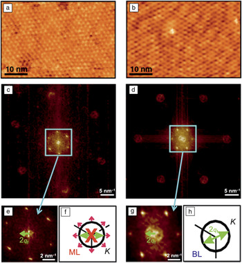
Because of the linear dispersion of graphene, the electrons in graphene are described as massless Dirac fermions. Such fermions have electronic properties that can be visualized using STM. One such property is the suppression of electron backscattering in monolayer graphene, because the chirality of the electrons forbids reversal of their crystal momentum in a single scattering event.Reference Brihuega, Mallet, Bena, Bose, Michaelis, Vitali, Varchon, Magaud, Kern and Veuillen61, Reference Ando62 In Figure 6, this effect is shown for epitaxial graphene on SiC(0001). At low voltage biases (i.e., energies close to the Fermi level), the variations in the topographical features are similar to the changes in the DOS. To visualize the change in wave vectors of the electrons scattering off subsurface impurities and point defects on the graphene surface, Fourier transformation of the STM images in Figure 6a–b from real-space coordinates to reciprocal-space coordinates was carried out, as shown in Figure 6c (monolayer) and 6d (bilayer).The differences in appearance are immediately apparent.
(a–b) Low-bias STM images of (a) monolayer (ML) and (b) bilayer (BL) terraces. (c–d) Two-dimensional fast Fourier transform maps of the images in (a) and (b), respectively, illustrating the change in wave vectors of the scattered electrons. The six prominent spots arise from the reconstruction in the buffer layer. (e) Central region of (c), showing no intravalley-backscattering-related ring. (f) Intravalley backscattering is forbidden in ML graphene, because the pseudospin (pink arrows) is inverted for states on opposite sides of the constant-energy contour of the electron. (g) Central region of (d), showing a clear ringlike feature of radius 2q f related to intravalley backscattering, which is allowed in the BL. q f is the wave vector of the scattering electron with respect to the K point of the Brillouin zone. (h) Schematic of intravalley backscattering for BL graphene. Reproduced with permission from Reference Reference Brihuega, Mallet, Bena, Bose, Michaelis, Vitali, Varchon, Magaud, Kern and Veuillen61. ©2008, American Physical Society.

For monolayer graphene (Figure 6e), the central circle observed for bilayer graphene (Figure 6g) is absent. This absence demonstrates the suppression of intravalley backscattering that occurs in monolayer graphene, which is attributed to the electronic chirality associated with the Dirac cones, as shown in Figure 6f and 6h. For monolayer graphene in Figure 6f, the pseudospins at opposite ends of the constant-energy contour are the inverse of each other. Therefore, the overlap between the backscattered electron waves and the incident wave is zero, resulting in the suppression of intravalley backscattering. This suppression does not occur for bilayer graphene, as shown in Figure 6g. Hence, a central ring of radius 2q f is observed that results from the intravalley backscattering of bilayer graphene electrons with a change in electron wave vector from +q f to –q f, as depicted in Figure 6h. For a more in-depth discussion of the other features related to intervalley scattering, please refer to the article by Brihuega et al.Reference Brihuega, Mallet, Bena, Bose, Michaelis, Vitali, Varchon, Magaud, Kern and Veuillen61
Modification of graphene
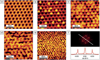
Local modifications of graphene, such as addition of defectsReference Tapaszto, Dobrik, Lambin and Biro57, Reference Yazyev and Helm63–Reference Wang, Huang, Song, Zhang, Ma, Liang and Chen66 and atomicReference Balog, Jørgensen, Nilsson, Andersen, Rienks, Bianchi, Fanetti, Lægsgaard, Baraldi, Lizzit, Sljivancanin, Besenbacher, Hammer, Pedersen, Hofmann and Hornekær42, Reference Tapaszto, Dobrik, Lambin and Biro57, Reference Guisinger, Rutter, Crain, First and Stroscio67–Reference Hupalo, Liu, Wang, Lu, Yao, Ho and Tringides78 and molecularReference Barja, Garnica, Hinarejos, Vázquez de Parga, Martín and Miranda43, Reference Hossain, Walsh and Hersam60, Reference Choi, Lee, Kim, Kim and Kim79–Reference Wang and Hersam85 adsorption, have been performed to alter its properties, for example, doping or opening a bandgap. Such effects can be characterized using STM. An example is the selective adsorption of hydrogen atoms on epitaxial graphene on Ir(111).Reference Balog, Jørgensen, Nilsson, Andersen, Rienks, Bianchi, Fanetti, Lægsgaard, Baraldi, Lizzit, Sljivancanin, Besenbacher, Hammer, Pedersen, Hofmann and Hornekær42 As discussed previously for Ru(0001), because of the lattice mismatch between graphene and the metal, a moiré pattern is observed (Figure 7a) before any hydrogen exposure.
STM images of hydrogen adsorbate structures following and preserving the moiré pattern of graphene on Ir(111). (a) Clean graphene on Ir(111). (b–e) Graphene exposed to atomic hydrogen for (b) less than 15 s, (c) 15 s, (d) 30 s, and (e) 50 s, showing the hydrogen structures increasingly decorating the bright parts of the moiré pattern with increasing hydrogen dose. (f) Top: Fourier transform of the image in (e), confirming that the hydrogen adsorbate structures preserve the moiré periodicity. Bottom: Line profile through the Fourier transform along the line in the top panel. The separation of the peaks corresponds to a real-space distance of 21.5 Å = 25 Å × cos(30°), confirming the moiré superlattice periodicity. Reproduced with permission from Reference Reference Balog, Jørgensen, Nilsson, Andersen, Rienks, Bianchi, Fanetti, Lægsgaard, Baraldi, Lizzit, Sljivancanin, Besenbacher, Hammer, Pedersen, Hofmann and Hornekær42. ©2010, Nature Publishing Group.

In Figure 7b, as atomic hydrogen is introduced, the hydrogen atoms selectively adsorb on the bright spots (high points) of the moiré pattern. At higher coverage, they form ringlike structures decorating the superlattice but still adsorb only on the bright areas of the moiré superlattice, as shown in Figure 7c–e. A Fourier transformation of the image in Figure 7e, shown in Figure 7f, confirms this selective adsorption, as the peak separation distance matches the moiré periodicity. Such a patterned adsorption of hydrogen has a significant effect on the electronic structure of graphene. Angle-resolved photoemission spectroscopy measurements revealed that the selective adsorption opens a bandgap of at least 0.45 eV because of the quantum confinement of the electrons in grapheneReference Balog, Jørgensen, Nilsson, Andersen, Rienks, Bianchi, Fanetti, Lægsgaard, Baraldi, Lizzit, Sljivancanin, Besenbacher, Hammer, Pedersen, Hofmann and Hornekær42 (also see the article in this issue by Conrad and Hicks).
In addition to modification through atomic or molecular adsorption, intercalation of epitaxial graphene to introduce novel elements between the graphene and the underlying substrate has been demonstrated. Hydrogen,Reference Riedl, Coletti, Iwasaki, Zakharov and Starke14, Reference Riedl, Coletti and Starke15, Reference Hiebel, Mallet, Veuillen and Magaud86–Reference Virojanadara, Yakimova, Zakharov and Johansson88 oxygen,Reference Sutter, Sadowski and Sutter89, Reference Oida, McFeely, Hannon, Tromp, Copel, Chen, Sun, Farmer and Yurkas90 metals,Reference Huang, Pan, Pan, Gao, Xu, Que, Zhou, Wang, Du and Gao44, Reference Jin, Fu, Mu, Tan and Bao46, Reference Cranney, Vonau, Pillai, Denys, Aubel, De Souza, Bena and Simon91–Reference Premlal, Cranney, Vonau, Aubel, Casterman, De Souza and Simon94 fluorine,Reference Wong, Huang, Wang, Cao, Qi, Santoso, Chen and Wee9, Reference Walter, Jeon, Bostwick, Speck, Ostler, Seyller, Moreschini, Kim, Chang, Horn and Rotenberg95 and even moleculesReference Varykhalov, Gudat and Rader96 can be intercalated between epitaxial graphene and its substrates. Modification of the graphene–substrate interface on SiC(0001) occurs when the new species migrates to and reacts with the silicon bonds holding the buffer layer to the substrate, releasing this layer to form graphene (see the article in this issue by Nyakiti et al.). The reacted layer then acts as the new interface. This interface could result in light p-type doping for the as-released graphene when less electronegative elements such as hydrogen are usedReference Poon, Chen, Wee and Tok29 or in a strongly p-doped layer when strongly electron-withdrawing elements such as fluorine are introduced.Reference Walter, Jeon, Bostwick, Speck, Ostler, Seyller, Moreschini, Kim, Chang, Horn and Rotenberg95n-Doped graphene layers formed by intercalating lithium atoms have also been reported.Reference Virojanadara, Watcharinyanon, Zakharov and Johansson92
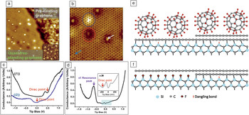
Figure 8 demonstrates fluorine intercalation using adsorbed C60F48 molecules as a source of fluorine.Reference Wong, Huang, Wang, Cao, Qi, Santoso, Chen and Wee9 The epitaxial graphene surface prior to intercalation has both a buffer layer and a graphene monolayer. C60F48 molecules are deposited, and the sample is annealed, giving the structure shown in Figure 8a. The absence of the underlying buffer layer confirmed that intercalation took place. Spectra ((1)) and ((2)) in Figure 8c correspond to the pristine monolayer epitaxial graphene and the intercalated graphene, respectively. The Dirac point has shifted to the Fermi level, because of the elimination of the buffer layer and the associated charge transfer from it. In Figure 8b, the small numbers of protrusions on the intercalated graphene are attributed to fluorine adatoms. STS performed over the protrusions indicated a resonance peak attributable to the influence of an electronegative potential exerted by the adatom on graphene. Graphene at these points is slightly p-doped, reflecting the electronegative adatom potential. The intercalation process is schematically illustrated in Figure 8e–f.
(a) STM image (20 nm × 20 nm) showing an intercalation-induced quasi-free-standing graphene monolayer joined continuously with a pre-existing graphene monolayer. Inset: High-resolution 8 × 8 nm2 STM image of clean EG revealing a reconstructed underlying buffer layer. (b) STM image (7 nm × 7 nm) of the intercalated surface. (c) Averaged dI/dV spectra recorded on ((1)) pre-existing graphene and ((2)) decoupled graphene at points away from the protrusion, such as that indicated by the blue arrow in (b). (d) dI/dV spectrum recorded over protrusions on decoupled graphene, as indicated by the white arrow in (b). In (d), the resonance peak is attributed to the effect of an electronegative fluorine atom. (e–f) Schematic models describing (e) C60F48 molecules deposited on a surface having a buffer layer everywhere and a region with an additional monolayer of graphene and (f) the continuous surface of a quasi-free-standing graphene monolayer and a nonintercalated graphene monolayer on a buffer layer after annealing at both 150°C and 850°C. Reproduced with permission from Reference Reference Wong, Huang, Wang, Cao, Qi, Santoso, Chen and Wee9. ©2011, American Chemical Society.

Conclusions
Scanning tunneling microscopy (STM) and scanning tunneling spectroscopy (STS) measurements allow for the characterization of topological and electronic properties of graphene on the local scale that macroscopic tools might fail to detect. STM can be used to determine the number of graphene layers, as well as defects, rotational disorder between graphene layers, and mismatch between graphene and its substrate. Modification of graphene at the local scale can have a significant effect on the attributes of the entire graphene layer. Therefore, STM is an atomically precise characterization tool for understanding the properties of pristine and modified graphene.
Acknowledgments
S.L.W. thanks NGS for a scholarship. The authors acknowledge financial support from NRF-CRP Grants R-144-000-295-281 “Novel 2D materials with tailored properties—Beyond graphene” and R-143-000-360-281 “Graphene Related Devices and Materials” and NUS YIA Grant R143-000-452-101.