INTRODUCTION
For over a century, the important role that the climate plays in the geographical distribution of the world's ecosystems and of the wildlife they support has been documented. It is now quite evident that the climate these species depend upon is changing. Climate variability and change, in fact, affect biomass in a number of ways, including shifts in species distribution. As local conditions change, new species may join communities while others may disappear from them or change in their relative and absolute abundances (Lemoine & Boehning-Gaese, Reference Lemoine and Boehning-Gaese2003; Bush et al., Reference Bush, Silman and Urrego2004; Genner et al., Reference Genner, Sims, Wearmouth, Southall, Southward, Henderson and Hawkins2004). Such changes, particularly in megafauna, can, in turn, lead to changes in species diversity, patterns of energy and, in the most extreme cases, alterations to entire ecosystems (Jackson & Sala, Reference Jackson and Sala2001). These ecological responses to changes in climate have important implications, given historical and continuing human-induced changes in the global climate. Recently, increasing attention has been given to large-scale patterns of climate variability that generate marked ecological impacts on interannual and longer time scales. Some evidence has been provided about the relevance of such large scale climatic phoenomena for the dynamics of different terrestrial and marine populations (Ottersen et al., Reference Ottersen, Planque, Belgrano, Post, Reid and Stenseth2001; Stenseth et al., Reference Stenseth, Mysterud, Ottersen, Hurrell, Chan and Lima2002). On the contrary, much fewer are the studies that have provided similar evidence on local or regional scales. Most measures of local climate used by ecologists fail to capture the complex associations between weather and the ecological process; time lags in the species responses to local climate coupled with the nonlinear intrinsic nature of population dynamics, make it extremely difficult to understand the patterns (Hallet et al., 2004). On the contrary large-scale indices of climate, spanning several months and considering wider areas of influence are less disturbed by local variability and very often outperform local climatic factors (Hallet et al., 2004). However, an understanding of the mechanism by which climate influences population ecology on regional and local scales is important.
The aim of this study was to assess if sea surface temperature does affect cetacean distribution in the western Ligurian Sea. Relationships with temperature have been investigated for: striped dolphin (Stenella coeruleoalba), fin whale (Balaenoptera physalus) and sperm whale (Physeter macrocephalus).
MATERIALS AND METHODS
Study area
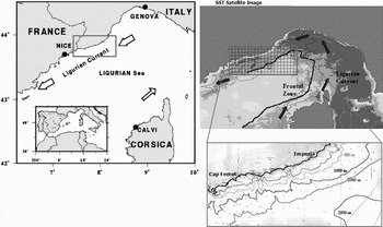
The study area is included within the Ligurian Sea Sanctuary for Cetaceans. In this area, the combined effect of the peculiar submarine topography, which is extremely complex and heterogeneous, and the influence on water masses of the changeable wind and current regimes creates very high levels of primary productivity (Macquart-Moulins & Patriti, Reference Macquart-Moulins and Patriti1996; Gaudy & Champalbert, Reference Gaudy and Champalbert1998; Lacroix & Grégoire, Reference Lacroix and Grégoire2002). All cetaceans regularly observed in the Mediterranean Sea can be found in this region (Notarbartolo di Sciara et al., Reference Notarbartolo di Sciara, Agardy, Hyrenbach, Scorazzi and Van Klaveren2007). The major physical factors affecting this region are the north-western winds. Mostly during winter, they strongly influence coastal waters, the fate of the Rhône plume, the ‘Liguro-Provençal Current’ with its associated thermal front which flows south-westerly along the continental slope (Conan & Millot, Reference Conan and Millot1995). The structure of the Liguro-Provençal Current remarkably changes seasonally. In fact, during winter the flux is at its maximum, becoming thicker and narrower and flowing closer to the slope. In summer, the Current is relatively wide and shallow, and it displays reduced mesoscale variability (Millot, Reference Millot1987). If during winter the ‘mistral’ winds channelled down the Rhône valley to the Gulf of Lions cool the surface water, during the summer season the wind regime can be much more changeable strongly affecting the circulation of water masses. Strong gusts of seawards wind (mostly north-westerly but also north-easterly), in fact, generate an offshore current in the superficial layers and a coastal upwelling carrying off the shelf into deeper waters (Macquart-Moulins & Patriti, Reference Macquart-Moulins and Patriti1996). The study area is approximately encompassed between the longitude of Cap Ferrat (7.33°E), close to the French/Italian border, and the longitude/latitude of Imperia (8.02°E 43.80°N) and the 50-m and 2000/2500-m depth contours (see Figure 1). It includes a significant portion of the continental slope area. The study area was divided into 189 cells, each measuring 3 × 3 nautical miles by means of a global information system routine (ESRI Arcview 3.2). The grid size chosen was large enough to avoid spatial autocorrelation (see the corresponding paragraph in the Results section).
Study area.

Cetacean sightings
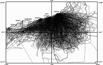
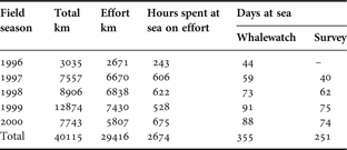
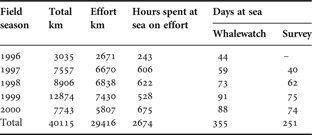
The study was focused on fin whales (Balaenoptera physalus), striped dolphins (Stenella coerulealba) and sperm whales (Physeter macrocephalus), since preliminary investigations had shown that these species might be affected by the thermal front variability in the area (Azzellino et al., in press). Sighting data collected during shipboard surveys conducted from 1996 to 2000 during the summer season were considered. Surveys, conducted from the beginning of June to the end of September, covered approximately an average of 10,000 km of search effort per year and an area of about 3000 km2. A total of 564 striped dolphin sightings, 119 fin whale sightings and 37 sperm whale sightings were considered. Data were obtained by two different platforms, one of the two being a whale-watching boat (see Table 1). The observation point on both platforms was about 4 m above the sea surface level. Aboard the whale-watching boat, experienced observers (at least one trained biologist) guaranteed the reliability of the species identification and of the corresponding data collection. Sighting data were collected roughly along north to south transects. Transects did not follow a systematic design with random probability sampling, but were designed as triangles to cross depth contours as perpendicularly as possible and to cover as much of the area as possible, although it was not covered homogeneously (Figure 2). Once the animals were located, transects were interrupted and data were collectected as long as the animals were in sight. A ‘sighting’ was deemed as a group of animals of the same species seen at the same time showing similar behavioural characteristics. Observations were made in flat seas and calm weather, defined as ‘favourable conditions’, and ceased when wind exceeded 3 on the Beaufort scale (wind speed: 5.4 m s−1). Searching and sea state status were recorded every 60 minutes, or more frequently if changes in conditions occurred. All the data were recorded through the IFAW-LOGGER Data Logging software.
Map showing the shipboard transects carried out from 1996 to 2000 in the study area.

Effort statistics for the two platforms.
Sea surface temperature (SST) data
A time series of monthly SST images was considered. Each image is characterized by a spatial resolution of 1.1 km. The data set used is an AVHRR MCSST product from the German Aereospace Research Centre–DLR (http://isis.dlr.de). Twenty SST monthly images (i.e. 4 images per research season) from June to September in the period 1996–2000 were used. The study area was divided into cells of 3×3 nautical miles and the species presence was associated to remotely-sensed SST data. For every cell the SST mean, standard deviation (SD) and coefficient of variance (CV) were calculated. Besides the simple SST statistics described, the deviation from the monthly average (i.e. the averages of the cell SST values calculated for every year–month period over the whole grid) was used as a predictor.
Statistical methods
A presence/absence (cells with sightings vs cells without sightings) binary logistic regression analysis (Afifi & Clark, Reference Afifi and Clark1996; Guisan & Zimmermann, Reference Guisan and Zimmermann2000) was used to correlate the species presence to SST cell features. To balance the number of absence observations, presence data were weighted on the basis of encounter rates. The year and the month of the fieldwork season were both considered as potential predictors to account for the interannual and seasonal variability. In order to select the best set of predictors, a forward stepwise method was used. So each predictor is tested for entry into the model one by one, based on the significance level of the score statistic. After each entry, variables that are already in the model are tested for possible removal, based on the significance of the Wald statistic (Hosmer & Lemeshow, Reference Hosmer and Lemeshow2000). The variable with the largest probability greater than the specified threshold value is removed, and the model is re-estimated. The procedure stops when no more variables meet entry or removal criteria or when the current model is the same as a previous model.
RESULTS
Spatial autocorrelation
According to Legendre et al. (Reference Legendre, Dale, Fortin, Gurevitch, Hohn and Myers2002) the presence of spatial correlation may disturb tests of significance for correlation or regression, when both the animal response variable and the environmental predictor are spatially autocorrelated. Therefore, in order to test whether the grid size was large enough to avoid the bias due to autocorrelation, the presence data of the different species were analysed by means of Moran's I index (Boots & Getis, Reference Boots and Getis1988). According to these authors, this index is a global ‘measure of the correlation among neighbouring observations in a pattern’ and it can be expressed through the following formula:
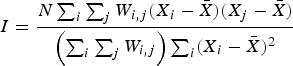
where N is the number of cases, X i is the variable value at a particular location, X j is the variable value at another location  is the mean of the variable and W ij is a weight applied to the comparison between location i and location j.
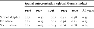
Moran's I index is similar to the Pearson's coefficient of correlation: it varies between –1.0 and +1.0. Moran's I was computed by year on the basis of the cell encounter rates using the MapStat extension to ArcView. Table 2 shows the Moran's I indices calculated for all the species considered.
Global Moran's I index for spatial autocorrelation. The Moran's I are calculated by year for every species on the basis of the cell encounter rate.
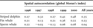
Moran's I indices ranged between −0.13 and 0.48 with a mean of 0.21 indicating that presence cells (i.e. encounter rates) are affected by a very weak spatial autocorrelation. So it can be concluded that the grid we used has the appropriate size.
Relationships with temperature
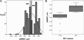
The stepwise logistic regression analysis was applied for all the species using the following SST descriptors: the cell SST mean, the cell SST, SD and the CV. Furthermore, deviations from the seasonal average (i.e. the monthly average calculated over the whole grid considering the whole study period) have been considered. Every SST value, calculated for the specific ‘month–year’ period (e.g. July 1997, August 2000 etc.) was evaluated as deviation from the monthly average. As Figure 3 shows, such a variable, named ‘diffSST_ave’, is mostly positive and its distribution could be divided into classes using the median (2.35°C deviation from the seasonal average) as a splitting criterion. However, in order to make the predictor easier to understand the median of 2.35°C was rounded to 3.00°C. Therefore, a new dichotomous predictor was generated for every cell: ‘3degrsover’ or whether the specific cell had an SST value 3°C higher than the seasonal average or not.
Analysis of the cell deviations from the sea surface temperature (SST) seasonal average (i.e. average evaluated over the whole 1996–2000 period): (A) frequency distribution of the SST deviations from the seasonal average; and (B) box plots showing the distribution of SST deviations within the two classes created using the median as a splitting criterion (each box shows the median, quartiles and extreme values within a category).

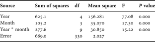
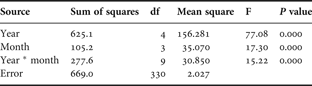
A two-way analysis of variance outlined that such deviations from the seasonal average are affected by interannual and monthly variability (P < 0.001, see Table 3). The ‘year ×month’ interaction term being also significant, it can be assumed that the monthly SST trend profiles were completely different from year to year. For this reason, the year and the month were both tested for entry in the stepwise procedure.
Two-way analysis of variance applied to diffSST_ave (deviations from the seasonal average). Both the year and the month gave significant results. The ‘year×month’ interaction term was significant as well.
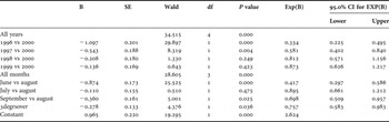
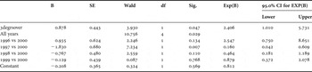
Although different SST features resulted to be alternatively included or excluded in the different developed models, only the ‘3degrsover’ predictor remains significant (P < 0.05) for all the species. Particularly, those ‘SST extreme values’ cells are avoided by striped dolphins and fin whales and preferred by sperm whales (see Tables 4–6).
Fin whale: results of the binary logistic regression analysis. Fin whale presence is inversely correlated with the cells with more than 3 degrees of deviation from the seasonal average.

B, unstandardized regression coefficient estimates; SE, standard error of the coefficient estimates; Exp(B), odds ratio (i.e. the ratio-change in the odds of the event of interest for a one-unit change in the predictor) and 95% confidence interval (CI) for Exp(B).
Striped dolphin: results of the binary logistic regression analysis. Striped dolphin presence is inversely correlated with the cells with more than 3 degrees of deviation from the seasonal average. Presence/absence is affected by interannual and monthly variability.

B, unstandardized regression coefficient estimates; SE, standard error of the coefficient estimates; Exp(B), odds ratio (i.e. the ratio-change in the odds of the event of interest for a one-unit change in the predictor) and 95% confidence interval (CI) for Exp(B).
Sperm whale: results of the binary logistic regression analysis. Sperm whale presence is directly correlated with the cells with more than 3 degrees of deviation from the seasonal average. Presence/absence is affected by interannual variability.

B, unstandardized regression coefficient estimates, SE, standard error of the coefficient estimates; Sig., significance; Exp(B), odds ratio (i.e. the ratio-change in the odds of the event of interest for a one-unit change in the predictor) and 95% confidence interval (CI) for Exp(B).
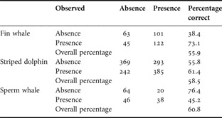
As shown in the confusion matrix (see Table 7) all the developed models are not able to correctly predict much higher than 60% of the overall presence/absence cells, however, fin whale and striped dolphin models predict more accurately the presence cells, whereas the sperm whale model classifies more accurately the absence cells.
Confusion matrix showing the logistic model classification performance.

DISCUSSION
In recent years increasing evidence for impacts on ecological processes of large scale climate variation has been provided in animal populations (e.g. Philander, Reference Philander1990; Stenseth et al., Reference Stenseth, Mysterud, Ottersen, Hurrell, Chan and Lima2002). Although individuals and populations experience climate locally through temperature, wind, currents, rain and snow changes, very often these meteorological and oceanographic features are governed by phenomena extending over much larger areas. The effect of such large scale phoenomena has been well documented (Stenseth et al., Reference Stenseth, Bjornstad, Falck, Fromentin, Gjosaeter and Gray1999; Ottersen et al., Reference Ottersen, Planque, Belgrano, Post, Reid and Stenseth2001). Climatic indices such as ENSO (i.e. El Niño–Southern Oscillation) and NAO (i.e. North Atlantic Oscillation) are probably the most well known examples of these large-scale ocean–atmosphere dynamics that generate impacts in both marine and terrestrial environments over a large part of the globe (Allan et al., Reference Allan, Lindesay and Parker1996; Post et al., Reference Post, Forchhammer and Stenseth1999). Although, large-scale indices were shown to have an effect, both direct and indirect, on terrestrial vegetation (Catchpole et al., Reference Catchpole, Morgan, Coulson, Freeman and Albon2000; Mysterud et al., Reference Mysterud, Stenseth, Yoccoz, Ottersen, Langvatn and Hurrell2003), herbivores and carnivores (Jewell et al., Reference Jewell, Milner and Morton1974; Post & Stenseth, Reference Post and Stenseth1999; Forchhammer et al., Reference Forchhammer, Clutton-Brock, Lindstrom and Albon2001), as well as on marine biology and fish stocks (Stenseth et al., Reference Stenseth, Bjornstad, Falck, Fromentin, Gjosaeter and Gray1999, Reference Stenseth, Ottersen, Hurrell, Mysterud, Lima, Chan, Yoccoz and Adlandsvik2003), no such evidence was provided between climate variation and the corresponding effect on populations, on local scale (Hallet et al., 2004). Very often, in fact, the underlying mechanisms of these phenomena remain unclear (Stenseth et al., Reference Stenseth, Ottersen, Hurrell, Mysterud, Lima, Chan, Yoccoz and Adlandsvik2003), in particular the effect on higher trophic levels, which would imply considering relationships that may not be linear, and therefore, even more difficult to understand (May, Reference May1986). Furthermore, there may be lags in the species responses to local climate (Hallet et al., 2004) which coupled with the potential non-linear population dynamics, make it even more difficult to comprehend the patterns. As far as cetaceans are concerned, with the exception of some polar species (De La Mare, Reference De La Mare1997; Laidre & Heide-Jørgensen, Reference Laidre and Heide-Jørgensen2005) relatively few studies have documented the effect of climate variation on cetacean species considering local scales (Lusseau et al., Reference Lusseau, Williams, Wilson, Grellier, Barton, Hammond and Thompson2004; MacLeod et al., Reference MacLeod, Bannon, Graham, Schweder, Learmonth, Herman and Reid2005). And it is reasonable to theorize that if cetaceans respond to climate change, since they are eurytherm, any response will be rather due to the indirect effect of climate change on the distribution of their prey. Anyway, SST is commonly considered among the potential predictors of cetacean distribution (e.g. Florez-Ramirez et al., 1996; Hastie et al., Reference Hastie, Swift, Slesser, Thompson and Turrell2005; Tynan et al., Reference Tynan, Ainley, Barth, Cowles, Pierce and Spear2005); thermal fronts and gradients, are known factors of influence for cetaceans (e.g. Doniol-Valcroze et al., Reference Doniol-Valcroze, Berteaux, Larouche and Sears2007). However, the mechanisms linking these variables to patterns of habitat selection are largely unknown and have begun to be investigated only recently (Croll et al., Reference Croll, Marinovic, Benson, Chavez, Black, Ternullo and Tershy2005; Doniol-Valcroze et al., Reference Doniol-Valcroze, Berteaux, Larouche and Sears2007). The interannual variability of the SST spatial patterns and the link of the surface patterns with the deeper layers of the water column is the reason why a simple cause–effect relationship with SST is difficult to find. Moreover, although studies on the relationship of some species with temperature and other correlated hydrologic features were conducted, very scarce indication about such influence of temperature on cetaceans is available for the Mediterranean area. Littaye et al. (Reference Littaye, Gannier, Laran and Wilson2004) used two different gradients as SST predictors on fin whales in the Mediterranean Sea: a spatial gradient calculated within the cell units between two points along the boat tracks and a temporal gradient between two successive 8-d periods. Therefore their choice was to use gradients instead of SST absolute values as predictors. Notwithstanding, the interannual variability is still appreciable in their models since the coefficients of partial correlation of the different SST predictors changed from year to year and among the different geographical provinces they were considering in their study. However, despite different temporal scale and the larger geographical resolution, Littaye and colleagues' results are consistent with what we found in a much smaller area using a monthly temporal resolution. The SST predictor we adopted in our study considers the deviation from a seasonal average calculated for the study period over the whole grid of analysis and this indicates that fin whales and striped dolphins respond to the spatial variability of the SST features and are both attracted by thermal anomalies (i.e. cells with SST values lower than the seasonal averages). In this respect, it is interesting that sperm whales presented a direct correlation with the SST predictor, showing a lower preference for those cells with the thermal anomaly.
It is well known that sperm whales in this area use preferentially the upper and lower slope waters that, especially during summer (Gannier et al., Reference Gannier, Drouot and Goold2002), are deeply influenced by the Liguro-Provençal thermal front, which flows south-westerly along the continental slope.
On the other hand, fin whales and striped dolphins, being much less related to the slope area and feeding mainly on the organisms inhabiting the first hundred metres below the surface, present a completely different response to the SST feature patterns. In conclusion, we believe that these preliminary insights highlight the need for a better understanding of the relationship of SST features with the species distribution. Since the relationship with SST features is significant at different spatial and temporal scales as the work of Littaye and colleagues demonstrates climatic changes will affect undoubtely the distribution of these species.
CONCLUSIONS
The SST features are a key factor for the habitat selection of fin whales, striped dolphins and sperm whales in the western Ligurian Sea. Logistic models, although not being particularly accurate in their predictions outlined the significant role of the SST features. Besides the generic cell SST statistics (i.e. mean, SD, CV), a deviation of 3°C from the seasonal average was found to be a significant predictor for all the considered species. Particularly, this analysis outlined that cells with such SST extreme values are either avoided by striped dolphins and fin whales or preferred by sperm whales. These results allow the conclusion that cetacean distribution in the western Ligurian Sea may change in response to climate variability. Further investigations spanning longer time periods are urgently needed to assess how climate changes will affect the structure of the cetacean communities living in this area.
ACKNOWLEDGEMENTS
We thank all the people (researchers, research assistants, collaborators, volunteers and undergraduate students) who contributed to the Tethys fieldwork campaigns. Enzo Barletta, Lucio Lessini, Ignazio Cavarretta and skippers of the vessels operated by Tethys Research Institute, have provided invaluable support in the fieldwork. Many thanks to Albert Sturlese, Barbara Nani, Marco Ballardini and all the bluWest staff. Thanks to the International Fund of Animal Welfare (IFAW) for the use of the software LOGGER and to Marina degli Aregai and Portosole for the logistic support.