



1. Introduction
1.1. Classification of aerofoil buffet and geometrical complexity
At certain combinations of free-stream Mach number
 $ (M_{\infty } )$
and angle of incidence
 $ (\alpha )$
, aerofoils in the transonic flow regime are susceptible to a self-sustained aerodynamic instability known as transonic aerofoil buffet (Lee Reference Lee1990). Buffet is characterised by low-frequency chordwise shock wave unsteadiness in the Strouhal number range
 ${\textit{St}}=({f^{*}c^{*}}/{u_{\infty }^{*})}\sim [0.05,0.1]$
, where
 $f$
is the frequency,
 $c$
is the aerofoil chord length,
 $u$
is the freestream velocity and is coupled to periodic separation and reattachment of the boundary layer (Lee Reference Lee2001). This phenomenon places limitations on the safe flight envelope of aircraft and remains an important topic in aerodynamics research (Giannelis et al. Reference Giannelis, Vio and Levinski2017). Due to its primary relevance in aerospace applications, the present work focuses on type II buffet, which refers to shock oscillations isolated to the suction side of asymmetric supercritical aerofoils at non-zero angles of attack (Giannelis et al. Reference Giannelis, Vio and Levinski2017). Numerous explanations have been proposed for the underlying mechanism, including feedback-loop models (Lee Reference Lee1990; Deck Reference Deck2005; Jacquin et al. Reference Jacquin, Molton, Deck, Maury and Soulevant2009; Hartmann et al. Reference Hartmann, Feldhusen and Shroder2013) and interpretations based on global instability (Crouch et al. Reference Crouch, Garbaruk, Magidov and Travin2009; Sartor et al. Reference Sartor, Mettot and Sipp2015). More recently, resolvent analysis of high-fidelity large-eddy simulation data has been used to relate the buffet dynamics to shock-induced separation height and pressure fluctuations around the shock wave (Iwatani et al. Reference Iwatani, Asada, Yeh, Taira and Kawai2023).
Transonic buffet (figure 1) has been investigated using configurations of varying geometrical complexity, which determines the extent to which two-dimensional (2-D) and three-dimensional (3-D) flow features can be captured. In addition to canonical 2-D chordwise shock oscillations, buffet has been shown to exhibit spanwise separation-bubble-induced distortion of the shock in unswept wide-span infinite wings (Lusher et al. Reference Lusher, Sansica and Hashimoto2025a ). These separation cells, or buffet cells, become unsteady and start travelling along the shock front on swept infinite wings (He & Timme Reference He and Timme2021; Lusher & Sansica Reference Lusher and Sansica2026) and finite wing configurations (Iovnovich & Raveh Reference Iovnovich and Raveh2015; Sugioka et al. Reference Sugioka, Koike, Nakakita, Numata, Nonomura and Asai2018, Reference Sugioka, Kouchi and Koike2022; Sansica et al. Reference Sansica, Hashimoto, Koike and Kouchi2022a ). In the context of numerical simulations, the degree of geometrical complexity is one aspect that limits the fidelity of the numerical methods that can be applied. The complexity can therefore range from purely 2-D simulations (Crouch et al. Reference Crouch, Garbaruk, Magidov and Travin2009; Kojima et al. Reference Kojima, Yeh, Taira and Kameda2020; Sansica et al. Reference Sansica, Loiseau, Kanamori, Hashimoto and Robinet2022b ), to 3-D simulations of spanwise homogeneous infinite wings (at different spanwise widths) (Deck Reference Deck2005; Garnier & Deck Reference Garnier and Deck2013; Ishida et al. Reference Ishida, Ishiko, Hashimoto, Aoyama and Takekawa2016; Fukushima & Kawai Reference Fukushima and Kawai2018; Memmolo et al. Reference Memmolo, Bernardini and Pirozzoli2018; Moise et al. Reference Moise, Zauner, Sandham, Timme and He2023; Lusher et al. Reference Lusher, Sansica and Hashimoto2024, Reference Lusher, Sansica and Hashimoto2025a ), individual isolated 3-D finite wings (Iovnovich & Raveh Reference Iovnovich and Raveh2015; Ohmichi et al. Reference Ohmichi, Ishida and Hashimoto2018) and full aircraft configurations (Sartor & Timme Reference Sartor and Timme2017; Masini et al. Reference Masini, Timme and Peace2020; Houtman et al. Reference Houtman, Timme and Sharma2023; Sansica & Hashimoto Reference Sansica and Hashimoto2023; Tamaki & Kawai Reference Tamaki and Kawai2024). Within this broad range of geometrical complexity and modelling approaches, a common and unifying feature of transonic buffet is the shock wave/boundary-layer interaction (SBLI) (Babinsky & Harvey Reference Babinsky and Harvey2011), whose dynamics ultimately governs the onset and characteristics of the unsteadiness.
1.2. Transonic shock wave/boundary-layer interactions
At unsteady buffet conditions, the SBLI couples the inviscid shock dynamics with a viscous boundary-layer response, giving rise to low-frequency shock motion and periodic separation and reattachment. The SBLIs involve a complex coupling between inviscid and viscous effects (Dolling Reference Dolling2001) over a range of spatio-temporal scales. The adverse pressure gradient imposed by the shock thickens the boundary layer and, for sufficiently strong interactions, leads to flow separation. Such separation causes increased drag, loss of lift and large-scale unsteadiness (Clemens & Narayanaswamy Reference Clemens and Narayanaswamy2014). At fixed free-stream conditions and Reynolds number, the ability of the boundary layer to resist separation is largely determined by the upstream boundary-layer state. Consequently, the influence of upstream boundary-layer conditions on SBLI behaviour and buffet dynamics is of central interest. Historically, SBLIs have been classified as laminar, transitional or turbulent based on the state of the boundary layer through the interaction (Gadd et al. Reference Gadd, Holder and Regan1954). In configurations with moving shocks and unstable separation bubbles, as in transonic buffet, this classification is commonly relaxed to focus on the boundary-layer state upstream of the SBLI (Moise et al. Reference Moise, Zauner and Sandham2022, Reference Moise, Zauner, Sandham, Timme and He2023).
(a) Schematic of transonic aerofoil buffet and associated SBLI; (b) example Mach number contours for a turbulent buffet ILES case from the present study.

1.3. Laminar and turbulent aerofoil buffet
Recent studies of laminar aerofoil buffet (Brion et al. Reference Brion, Dandois, Abart and Paillart2017; Dandois et al. Reference Dandois, Mary and Brion2018; Memmolo et al. Reference Memmolo, Bernardini and Pirozzoli2018; Brion et al. Reference Brion, Dandois, Mayer, Reijasse, Lutz and Jacquin2020; Moise et al. Reference Moise, Zauner and Sandham2022; Zauner et al. Reference Zauner, Moise and Sandham2022; Moise et al. Reference Moise, Zauner, Sandham, Timme and He2023; Polivanov & Sidorenko Reference Polivanov and Sidorenko2026) consider configurations that are initially laminar and transition to turbulence in the aft section of the aerofoil downstream of the SBLI. Laminar buffet is commonly defined as the case in which the boundary layer remains laminar from the leading edge to approximately the shock-foot location and no boundary-layer tripping is applied (Moise et al. Reference Moise, Zauner and Sandham2022). In contrast, turbulent buffet refers to cases in which the boundary layer is already fully turbulent upstream of the SBLI (Fukushima & Kawai Reference Fukushima and Kawai2018; Nguyen et al. Reference Nguyen, Terrana and Peraire2022; Sansica et al. Reference Sansica, Loiseau, Kanamori, Hashimoto and Robinet2022b ; Moise et al. Reference Moise, Zauner, Sandham, Timme and He2023; Lusher et al. Reference Lusher, Sansica and Hashimoto2024, Reference Lusher, Sansica and Hashimoto2025a ; Lusher & Sansica Reference Lusher and Sansica2026), typically enforced through turbulence modelling and/or boundary-layer tripping.
In general, dedicated investigations of aerofoil buffet contrasting varying upstream boundary-layer states are sparse within the literature. Previous studies of laminar and turbulent aerofoil buffet have only examined cases in which the upstream boundary-layer state is either nominally laminar or fully turbulent in front of the SBLI. Experimentally, Brion et al. (Reference Brion, Dandois, Abart and Paillart2017) compared laminar with tripped turbulent buffet at a Reynolds number of
 $\textit{Re}_c={\rho _{\infty }^{*} U_{\infty }^{*}c^{*}}/{\mu _{\infty }^{*}}=3\times 10^{6}$
, where
 $\rho_{\infty}$
is the free-stream density,
 $U_{\infty}$
is the free-stream velocity and
 $\mu_{\infty}$
is the free-stream viscosity. In the turbulent case, a standard low-frequency buffet mode was observed at
 ${\textit{St}}=0.07$
, whereas the laminar case exhibited only minor chordwise shock displacements together with energy content around
 ${\textit{St}}\approx 1$
, attributed to localised oscillation of the shock foot. Follow-up experiments on the same OALT25 aerofoil (Brion et al. Reference Brion, Dandois, Mayer, Reijasse, Lutz and Jacquin2020) identified similar higher-frequency energy content at
 ${\textit{St}}\approx 1.1$
, alongside a weaker low-frequency peak at
 ${\textit{St}}=0.05$
, with the higher-frequency mode attributed to the laminar separation-bubble dynamics.
Computational studies reported similar behaviour. Memmolo et al. (Reference Memmolo, Bernardini and Pirozzoli2018) simulated laminar buffet on the Dassault V2C aerofoil at
 $\textit{Re}_c=3\times 10^{6}$
, identifying both a low-frequency shock-oscillation mode at
 ${\textit{St}}\approx 0.1$
and a secondary peak at
 ${\textit{St}}\approx 1$
associated with Kelvin–Helmholtz vortex shedding in the separated region. Likewise, Dandois et al. (Reference Dandois, Mary and Brion2018) observed energy content at
 ${\textit{St}}\approx 1.2$
on the OALT25 geometry. These studies concluded that laminar buffet is governed by the dynamics of a laminar separation bubble, whereas turbulent buffet is associated with a global instability involving periodic separation and reattachment between the shock and trailing edge. These additional features and modes are commonly reported to be specific to, and defining characteristics of, laminar buffet (Dandois et al. Reference Dandois, Mary and Brion2018; Moise et al. Reference Moise, Zauner and Sandham2022; Zauner et al. Reference Zauner, Moise and Sandham2022; Moise et al. Reference Moise, Zauner, Sandham, Timme and He2023).
At more moderate Reynolds numbers (
 $\textit{Re}_c = 5\times 10^5$
), Moise et al. (Reference Moise, Zauner, Sandham, Timme and He2023) presented numerical comparisons between tripped and untripped buffet on the V2C profile. They reported sensitivity of buffet behaviour to the upstream boundary-layer state, with differences in shock topology between multiple (untripped) and single (tripped) shock configurations on the suction side of the aerofoil. Nevertheless, both tripped (
 ${\textit{St}}=0.13$
) and untripped (
 ${\textit{St}}=0.15$
) cases exhibited similar 2-D buffet frequencies, although the untripped case showed significantly stronger shock oscillations at a fixed free-stream Mach number. Intermediate (
 ${\textit{St}}\approx 0.5$
) and higher (
 ${\textit{St}}\approx 1$
) frequency content was also observed. Taken together, the above experimental and numerical studies (Brion et al. Reference Brion, Dandois, Abart and Paillart2017, Reference Brion, Dandois, Mayer, Reijasse, Lutz and Jacquin2020; Dandois et al. Reference Dandois, Mary and Brion2018; Moise et al. Reference Moise, Zauner, Sandham, Timme and He2023) compared laminar and turbulent buffet using a binary classification: either untripped (free-transition) boundary layers that remain laminar up to the shock foot and transition only within or downstream of the shock-induced separation bubble, or fully tripped configurations with a turbulent boundary layer upstream of the interaction. Cases in which the boundary layer undergoes partial transition upstream of the SBLI are not explicitly examined in these studies, and the sensitivity of buffet dynamics to intermediate upstream boundary-layer states therefore remains largely unexplored.
No attention has explicitly been given to buffet with transition occurring directly upstream of the SBLI. This region at the front of the shock foot has been identified as highly receptive by previous global-stability and resolvent analyses, through adjoint/sensitivity structures (Sartor et al. Reference Sartor, Mettot and Sipp2015; Paladini et al. Reference Paladini, Beneddine, Dandois, Sipp and Robinet2019a , Reference Paladini, Marquet, Sipp, Robinet and Dandoisb ) and resolvent forcing-mode support near the shock foot and upstream oblique region (Kojima et al. Reference Kojima, Yeh, Taira and Kameda2020; Iwatani et al. Reference Iwatani, Asada, Yeh, Taira and Kawai2023). The present contribution addresses this gap by simulating aerofoil buffet over a continuous range of laminar, transitional and turbulent upstream boundary-layer states using fourteen forcing levels. Our recent work (Lusher et al. Reference Lusher, Sansica and Hashimoto2024) identified a transitional case exhibiting characteristics distinct from both laminar and turbulent buffet. High-fidelity implicit large-eddy simulations (ILES; figure 1) and spectral proper orthogonal decomposition (SPOD) are applied. In addition to complementing existing numerical studies, this contribution also aims to support experimental investigations, for which accurate characterisation of the upstream boundary-layer state remains challenging.
Section 2 outlines the computational set-up. The classification of laminar, transitional and turbulent buffet interactions is presented in § 3, followed by analysis of the buffet global response (§ 4). The unsteady dynamics of the less-documented transitional interaction is characterised by means of SPOD in § 5 and the associated governing mechanisms are described in § 6. The paper concludes with a summary of the key findings and implications for buffet mechanisms.
2. Computational method
All simulations in this work were performed using the OpenSBLI open-source high-order compressible flow solver (Lusher et al. Reference Lusher, Jammy and Sandham2021). The most recent public release and associated verification and validation cases are described in Lusher et al. (Reference Lusher, Sansica, Sandham, Meng, Siklósi and Hashimoto2025b ). OpenSBLI has been cross-validated against multiple independently developed flow solvers by Chapelier et al. (Reference Chapelier2024) and has been used to generate high-Reynolds-number compressible turbulence datasets released on the JAXA direct numerical simulation (DNS) and NASA Turbulence Modelling Resource websites (Lusher & Coleman Reference Lusher and Coleman2022; Lusher et al. Reference Lusher, Sansica, Coleman and Spalart2026).
The governing equations are the non-dimensional compressible Navier–Stokes equations for an ideal gas. Conservation of mass, momentum and energy in the three spatial directions
 $x_i$
 $ (i=0,1,2 )$
yields a system of five partial differential equations for the density
 $\rho$
, velocity components
 $u_k$
, pressure
 $p$
, temperature
 $T$
and total energy
 $\rho E$
 \begin{align} \frac {\partial \rho }{\partial t} &+ \frac {\partial }{\partial x_k} \left (\rho u_k \right ) = 0, \\[-12pt]\nonumber \end{align}
 \begin{align} \frac {\partial }{\partial t}\left (\rho u_i\right ) &+ \frac {\partial }{\partial x_k} \left (\rho u_i u_k + p \delta _{ik} - \tau _{ik}\right ) = 0, \\[-12pt]\nonumber \end{align}
 \begin{align} \frac {\partial }{\partial t}\left (\rho E\right ) &+ \frac {\partial }{\partial x_k} \left (\rho u_k \left (E + \frac {p}{\rho }\right ) + q_k - u_i \tau _{ik}\right ) = 0, \end{align}
where
 $p$
is the pressure,
 $\delta_{i,k}$
is the kronecker delta, the heat flux
 $q_k$
and stress tensor
 $\tau _{ik}$
are defined as
 \begin{equation} q_k = \frac {-\mu }{\left (\gamma - 1\right ) M_{\infty }^{2} \textit{Pr} \textit{Re}}\frac {\partial T}{\partial x_k}, \quad \tau _{ik} = \frac {\mu }{\textit{Re}} \left (\frac {\partial u_i}{\partial x_k} + \frac {\partial u_k}{\partial x_i} - \frac {2}{3}\frac {\partial u_{\!j}}{\partial x_{\!j}} \delta _{ik}\right )\!. \end{equation}
Here,
 $\textit{Pr}$
,
 $\textit{Re}$
and
 $\gamma =1.4$
denote the Prandtl number, Reynolds number and ratio of specific heat capacities, respectively. Curvilinear coordinates are employed via a body-fitted mesh transformation. All variables are non-dimensionalised using the free-stream velocity, density and temperature
 $ (U^{*}_{\infty },\rho ^{*}_{\infty },T^{*}_{\infty } )$
. For a reference Mach number
 $M_{\infty }$
, the pressure–temperature relation is given by
 \begin{equation} p = \left (\gamma - 1\right ) \left (\rho E - \frac {1}{2} \rho u_i u_i\right ) = \frac {1}{\gamma M^{2}_{\infty }} \rho T. \end{equation}
Temperature-dependent viscosity is evaluated using Sutherland’s law
 \begin{equation} \mu (T) = T^{\frac {3}{2}}\frac {1 + C_{\textit{Suth}}}{T + C_{\textit{Suth}}}, \end{equation}
with
 $C_{\textit{Suth}}=T_{S}^{*}/T_{\infty }^{*}$
for
 $T_{S}^{*}=110.4\,\mathrm{K}$
and
 $T_{\infty }^{*}=273.15\,\mathrm{K}$
. The skin-friction coefficient is defined from the wall shear stress
 $\tau _w$
as
 \begin{equation} C_{\!f} = \frac {\tau _w}{0.5 \rho _{\infty }^{*} U_{\infty }^{*2}}. \end{equation}
The simulations are performed at a Reynolds number of
 $\textit{Re}_c=0.5\times 10^6$
based on the aerofoil chord length
 $c$
, and a transonic free-stream Mach number of
 $M_\infty =0.72$
. The lift coefficient is evaluated over the aerofoil surface with arc-length
 $s_{\textit{total}}$
as
 \begin{equation} C_L = \frac {1}{0.5\rho _{\infty }^{*} U_{\infty }^{*2}}\int _{s=0}^{s=s_{\textit{total}}} -S(p_w - p_{\infty }) \left |\cos (\theta ) \right | {\rm d}s, \end{equation}
where
 $\theta$
is the local surface inclination angle, and
 $p_w$
and
 $p_{\infty }$
are the wall and free-stream pressures, respectively. The sign term
 $S$
accounts for the orientation of the surface grid metrics. Surface distributions of
 $C_{\!f}$
and
 $C_p$
are averaged in time and in the spanwise direction unless otherwise stated. Aerodynamic force coefficients such as
 $C_L$
and
 $C_D$
are span averaged, and when also time averaged are denoted with an overbar.
As in our related aerofoil buffet studies (Lusher et al. Reference Lusher, Sansica and Hashimoto2024, Reference Lusher, Sansica and Hashimoto2025a ; Lusher & Sansica Reference Lusher and Sansica2026), high-fidelity ILES are performed by solving the governing equations (2.1)–(2.3) without an explicit subgrid-scale model. Fourth-order central differences are used for convective and diffusive terms, with the convective terms cast in a kinetic energy preserving cubic split form (Coppola et al. Reference Coppola, Capuano, Pirozzoli and de Luca2019) to improve nonlinear stability. Shock capturing is enabled via a hybrid method using a fifth-order weighted essentially non-oscillatory WENO-Z scheme (Borges et al. Reference Borges, Carmona, Costa and Don2008) coupled to the central differences, with additional numerical dissipation provided by a dispersion relation preserving DRP filter (Bogey & Bailly Reference Bogey and Bailly2004). Time advancement is performed using a fourth-order five-stage low-storage Runge–Kutta scheme. Full implementation details and resolution comparisons are provided in Lusher et al. (Reference Lusher, Sansica, Sandham, Meng, Siklósi and Hashimoto2025b ). Aerofoil-specific applications of this configuration include laminar buffet simulations on the V2C aerofoil profile (Lusher et al. Reference Lusher, Zauner, Sansica and Hashimoto2023) and turbulent buffet on the NASA-CRM aerofoil geometry (Lusher et al. Reference Lusher, Sansica and Hashimoto2024, Reference Lusher, Sansica and Hashimoto2025a ; Lusher & Sansica Reference Lusher and Sansica2026). The turbulent cases included cross-validation against buffet predictions from unsteady-Reynolds-averaged Navier-Stokes and global-stability analysis (Sansica & Hashimoto Reference Sansica and Hashimoto2023).
2.1. Geometry, mesh and flow conditions
Mesh generation is performed in the same manner as in Lusher et al. (Reference Lusher, Sansica and Hashimoto2024, Reference Lusher, Sansica and Hashimoto2025a
,
Reference Lusher, Sansica, Sandham, Meng, Siklósi and Hashimotob
). The selected aerofoil geometry is the 65 % semi-span station of the NASA-CRM wing (NASA-LaRC 2012), which is commonly used in transonic buffet research. Two-dimensional body-fitted structured C-meshes are generated in Pointwise™, with a total of 440 million grid points used in the present study. In the
 $\xi$
and
 $\eta$
directions around the aerofoil and normal to the surface, the aerofoil and wake blocks contain
 $ (2689,681 )$
and
 $ (801,681 )$
points, respectively. The pressure and suction sides are resolved with 500 and 2189 points in the streamwise direction to reflect the flow topology associated with type II buffet (Giannelis et al. Reference Giannelis, Vio and Levinski2017). The number of points allocated to the pressure side is comparable to similar aerofoil studies in the literature at higher Reynolds numbers than used here.
The
 $\xi$
distribution is refined between
 $0.1 \lt x \lt 0.6$
on the suction side to improve resolution of the transition, main shock wave and SBLI. The 3-D mesh is generated by extruding the 2-D grid in the spanwise direction with uniform spacing. A spanwise grid study at buffet conditions on the same NASA-CRM configuration was presented in Lusher et al. (Reference Lusher, Sansica and Hashimoto2024), and the ‘fine’ resolution of
 $N_z=150$
is adopted here, having been shown to provide grid-independent results at this Reynolds number. Directly upstream of the main shock at
 $x/c=0.425$
for the baseline turbulent case (
 $A$
-
 $7.50$
, table 1), the grid resolution corresponds to wall units of
 $ (\Delta x^{+}, \Delta y^{+}, \Delta z^{+} ) \approx (5.2,2.0,9.1 )$
. In the attached turbulent region downstream of the shock at
 $x/c=0.7$
, the baseline grid has local wall units of approximately
 $ (\Delta x^{+}, \Delta y^{+}, \Delta z^{+} ) \approx (2.9,0.9,3.7 )$
. The insensitivity of the present results to increased wall-normal refinement is demonstrated in Appendix B, where meshes with
 $\Delta y^{+} \approx 0.8$
and
 $\Delta y^{+} \approx 0.3$
at
 $x/c=0.425$
and
 $x/c=0.7$
, respectively, produce consistent buffet characteristics. Sensitivity to variations in the
 $(\xi$
–
 $\eta )$
resolution was also examined in Lusher et al. (Reference Lusher, Sansica and Hashimoto2024), with aerodynamic quantities and buffet frequency on coarser meshes remaining consistent with the finest grid. The total number of grid points is comparable to similar high-fidelity LES/ILES aerofoil buffet studies in the literature, including both laminar (Dandois et al. Reference Dandois, Mary and Brion2018; Moise et al. Reference Moise, Zauner and Sandham2022; Zauner et al. Reference Zauner, Moise and Sandham2022) and fully turbulent cases (Moise et al. Reference Moise, Zauner, Sandham, Timme and He2023).
Summary of the fourteen amplitude variations for the buffet cases simulated in this work. All cases are performed on the NASA-CRM profile at
 $AR=0.1$
,
 $\alpha = 5^{\circ }$
,
 $\textit{Re}_c=0.5\times 10^6$
, and free-stream
 $M_{\infty } = 0.72$
with zero sweep.

Table 1. Long description
A table summarizing amplitude variations for buffet cases simulated on the NASA-CRM profile. The table has 14 rows and 7 columns. Column headers are Case, Trip (percent U infinity), Interaction type, C L, C D p, C D f, C D, and St 2-D buffet. Row 1: Case A-0.00, Trip 0.00 percent, Interaction type Laminar, C L 0.986, C D p 0.0655, C D f 0.0051, C D 0.0705, St 2-D buffet 0.10. Row 2: Case A-0.05, Trip 0.05 percent, Interaction type Laminar, C L 0.938, C D p 0.0534, C D f 0.0044, C D 0.0579, St 2-D buffet 0.08. Row 3: Case A-0.50, Trip 0.50 percent, Interaction type Laminar, C L 1.039, C D p 0.0546, C D f 0.0041, C D 0.0587, St 2-D buffet 0.08. Row 4: Case A-1.50, Trip 1.50 percent, Interaction type Laminar, C L 1.070, C D p 0.0557, C D f 0.0062, C D 0.0619, St 2-D buffet 0.08. Row 5: Case A-2.25, Trip 2.25 percent, Interaction type Laminar, C L 1.032, C D p 0.0560, C D f 0.0063, C D 0.0622, St 2-D buffet 0.08. Row 6: Case A-2.50, Trip 2.50 percent, Interaction type Transitional, C L 1.078, C D p 0.0597, C D f 0.0065, C D 0.0661, St 2-D buffet 0.06. Row 7: Case A-2.65, Trip 2.65 percent, Interaction type Transitional, C L 1.101, C D p 0.0603, C D f 0.0067, C D 0.0670, St 2-D buffet 0.06. Row 8: Case A-2.70, Trip 2.70 percent, Interaction type Transitional, C L 1.136, C D p 0.0603, C D f 0.0067, C D 0.0670, St 2-D buffet 0.06. Row 9: Case A-2.75, Trip 2.75 percent, Interaction type Transitional, C L 1.145, C D p 0.0605, C D f 0.0068, C D 0.0673, St 2-D buffet 0.08. Row 10: Case A-3.00, Trip 3.00 percent, Interaction type Transitional, C L 1.117, C D p 0.0583, C D f 0.0072, C D 0.0655, St 2-D buffet 0.10. Row 11: Case A-3.25, Trip 3.25 percent, Interaction type Transitional, C L 1.080, C D p 0.0559, C D f 0.0074, C D 0.0633, St 2-D buffet 0.10. Row 12: Case A-5.00, Trip 5.00 percent, Interaction type Turbulent, C L 1.014, C D p 0.0526, C D f 0.0078, C D 0.0604, St 2-D buffet 0.08. Row 13: Case A-7.50, Trip 7.50 percent, Interaction type Turbulent, C L 0.998, C D p 0.0517, C D f 0.0080, C D 0.0597, St 2-D buffet 0.08. Row 14: Case A-10.0, Trip 10.00 percent, Interaction type Turbulent, C L 0.985, C D p 0.0513, C D f 0.0082, C D 0.0594, St 2-D buffet 0.08.
The inflow boundary is located
 $25c$
upstream of the aerofoil, with the outlet positioned
 $5c$
downstream. Sensitivity of the results to the downstream domain extent was previously assessed on the same configuration for outlet locations between
 $L_x=5c$
and
 $20c$
, with negligible effect on surface distributions and buffet characteristics (Lusher et al. Reference Lusher, Sansica and Hashimoto2024). Uniform unswept inflow conditions
 $(U_{\infty }=1)$
are prescribed, with the angle of attack imposed by rotating the aerofoil within the mesh. The spanwise domain width is set to
 $L_z=0.1c$
, which was shown to be sufficient to obtain domain-independent results for the 2-D buffet shock-oscillation mode (Lusher et al. Reference Lusher, Sansica and Hashimoto2024). A fixed non-dimensional time step of
 $\Delta t=5\times 10^{-5}$
is used for all cases. Insensitivity of the results to the selected time-step value is reported in Appendix A.
The baseline angle of attack is
 $\alpha = 5^{\circ }$
, which lies within the active buffet envelope for the flow conditions considered. Buffet onset on this geometry was previously identified at
 $\alpha = 4.5^{\circ }$
via global-stability analysis (Lusher et al. Reference Lusher, Sansica and Hashimoto2024). The flow is initialised from uniform free-stream conditions and advanced for 15 convective time units to establish the low-frequency buffet unsteadiness. After discarding the initial transient, a further 100 convective time units are simulated for all cases to capture multiple buffet cycles (figure 10
a) and enable the modal analysis presented in § 5. Each 440 million cell simulation required approximately 19 days on 20 NVIDIA V100 GPUs. The fourteen cases performed correspond to a total cost of 127 680 GPU-hours (equivalent to
 $7.44\times 10^{7}$
A64FX CPU-core-hours).
2.2. Numerical boundary-layer tripping
Boundary-layer tripping is routinely applied in simulations and wind tunnel experiments to obtain turbulent boundary layers at achievable Reynolds numbers. In the present study, numerical tripping is implemented using a time-varying, spanwise-modulated blowing/suction strip located near the leading edge of the aerofoil. The forcing strip is centred at
 $x/c=0.1$
on both the suction and pressure sides, consistent with its placement in wind tunnel experiments at JAXA on the same profile (Sugioka et al. Reference Sugioka, Kouchi and Koike2022). The forcing is applied to the wall-normal velocity component and scaled by the wall density to impose the corresponding momentum and total energy at the wall, while regions outside the forcing strip are treated with isothermal no-slip boundary conditions. The forcing follows a modified form of that proposed by Moise et al. (Reference Moise, Zauner, Sandham, Timme and He2023)
 \begin{equation} \rho v_w= \rho _w \sum _{i=1}^3 A \exp \left (-\frac {\left (x-x_t\right )^2}{2 \sigma ^2}\right ) \sin \left (\frac {k_i z}{0.05c}\right ) \sin \left (\omega _i t+\varPhi _i\right )\!, \end{equation}
where
 $t$
denotes simulation time,
 $x_t$
the trip location and
 $\sigma =0.00833$
the Gaussian width. The three modes
 $ (0,1,2 )$
have spatial wavenumbers
 $k_i= (6\pi ,8\pi ,8\pi )$
, phases
 $\varPhi _i= (0,\pi ,-\pi /2 )$
and temporal frequencies
 $\omega _i= (26,88,200 )$
. The same forcing strategy has been used in our recent aerofoil buffet studies (Lusher et al. Reference Lusher, Sansica and Hashimoto2024, Reference Lusher, Sansica and Hashimoto2025a
). Fourteen forcing amplitudes in the range
 $A=[0,10]\,\%\,U_\infty$
are considered (table 1) to systematically vary the upstream boundary-layer state. The classification of the interaction type for each case is given in § 3.1, based on a consistent set of boundary-layer diagnostics including skin friction, integral quantities (displacement and momentum thickness and shape factor), mean streamwise velocity profiles and root-mean-square velocity fluctuations, all evaluated upstream of the main interaction (figures 2–7).
2.3. Spectral proper orthogonal decomposition methodology
Modal decomposition methods have been widely applied to the analysis of unsteady fluid flows (Taira et al. Reference Taira, Brunton, Dawson, Rowley, Colonius, McKeon, Schmidt, Gordeyev, Theofilis and Ukeiley2017), including transonic buffet in recent years (Moise et al. Reference Moise, Zauner and Sandham2022, Reference Moise, Zauner, Sandham, Timme and He2023; Lusher et al. Reference Lusher, Sansica and Hashimoto2025a ; Ohmichi & Sugioka Reference Ohmichi and Sugioka2025; Lusher & Sansica Reference Lusher and Sansica2026). In this work, the frequency-resolved SPOD method (Towne et al. Reference Towne, Schmidt and Colonius2018) is used to decompose the flow into orthogonal modes ranked by their energy content in the frequency domain. Here, SPOD is employed to identify the spatial structure and physical origin of dominant unsteady modes present in the flow, and to support their physical interpretation in the context of buffet dynamics.
The open-source PySPOD library (Rogowski et al. Reference Rogowski, Yeung, Schmidt, Maulik, Dalcin, Parsani and Mengaldo2024) is used to perform the analysis. Application of SPOD to OpenSBLI data has been demonstrated previously in Hamzehloo et al. (Reference Hamzehloo, Lusher and Sandham2023) and Lusher et al. (Reference Lusher, Sansica, Sandham, Meng, Siklósi and Hashimoto2025b
). In the present work, side
 $x$
–
 $y$
plane data (at
 $z=L_z/2$
) and near-wall fields are sampled at intervals of
 $\Delta T_{\textit{SPOD}} = 1000\Delta t$
, providing a maximum resolvable Strouhal number of
 ${\textit{St}}=10$
, which is sufficient for the range of unsteady phenomena encountered in buffet (Moise et al. Reference Moise, Zauner, Sandham, Timme and He2023). The data are divided into three to nine segments with 50 % overlap, with a Hann window applied to each segment. Unless otherwise stated, only the leading SPOD mode at each frequency is considered and compared with the power spectral density of lift-coefficient fluctuations. The present SPOD methodology has been applied previously to transonic buffet in Lusher et al. (Reference Lusher, Sansica and Hashimoto2025a
,Reference Lusher, Sansica, Sandham, Meng, Siklósi and Hashimoto
b
) and Lusher & Sansica (Reference Lusher and Sansica2026).
3. Characterisation of buffet for different interaction types
Instantaneous streamwise velocity
 $(x,z)$
contours at a height of
 $y=0.003c$
above the suction-side surface. Displaying representative (a) laminar (A-0.50), (b) transitional (A-2.75) and (c) turbulent (A-7.50) cases when the shock is in the same approximate location. Regions of flow reversal
 $(u \lt 0)$
are outlined in white.

Figure 2. Long description
Panel A: A heat map displaying streamwise velocity contours for a laminar flow case (A-0.50). The x-axis represents the horizontal distance, and the y-axis represents the streamwise velocity. The color scale ranges from -0.8 to 1.8, with darker colors indicating lower velocities and lighter colors indicating higher velocities. Regions of flow reversal are outlined in white. Panel B: A heat map displaying streamwise velocity contours for a transitional flow case (A-2.75). The x-axis represents the horizontal distance, and the y-axis represents the streamwise velocity. The color scale ranges from -0.8 to 1.8, with darker colors indicating lower velocities and lighter colors indicating higher velocities. Regions of flow reversal are outlined in white. Panel C: A heat map displaying streamwise velocity contours for a turbulent flow case (A-7.50). The x-axis represents the horizontal distance, and the y-axis represents the streamwise velocity. The color scale ranges from -0.8 to 1.8, with darker colors indicating lower velocities and lighter colors indicating higher velocities. Regions of flow reversal are outlined in white.
A summary of the present simulations is shown in table 1. The laminar, transitional and turbulent interactions are classified for three representative cases using quantitative boundary-layer metrics and flow visualisations in § 3.1, with the corresponding impact on buffet characteristics shown in § 3.2. Each interaction class is then examined in detail in §§ 3.3–3.5 over multiple forcing levels per regime.
3.1. Classification of interaction types based on upstream boundary-layer state
Figure 2 shows instantaneous contours of the streamwise velocity in the
 $x-z$
plane at a fixed wall-normal height of
 $y=0.003c$
for three representative cases: A-0.50 (laminar), A-2.75 (transitional) and A-7.50 (turbulent). Only the suction-side surface is shown (see the
 $(x,y)$
side view in figure 1). The snapshots are selected such that the shock is located at approximately the same chordwise position in all three cases. For the initial classification in this section, the weakly forced A-0.50 case (table 1) is selected as a representative laminar reference. Although weaker forcing levels (A-0.05) and the fully untripped case (A-0.00) also remain laminar upstream of the interaction, A-0.50 provides a clearer reference state with a more consistent shock topology. A detailed comparison between A-0.50, A-0.05 and A-0.00 is therefore deferred to the laminar buffet discussion in § 3.4.
The instantaneous fields reveal a clear qualitative distinction between the three upstream boundary-layer states as the forcing amplitude is varied. The A-0.50 case exhibits a smooth, largely spanwise-uniform laminar boundary layer upstream of the SBLI. Weak spanwise perturbations associated with the imposed forcing are visible immediately upstream of the separation line; however, these disturbances do not lead to transition prior to the interaction. Instead, transition occurs only when perturbations are amplified within the shock-induced separated shear layer, consistent with observations in other laminar SBLI studies (Sansica et al. Reference Sansica, Sandham and Hu2014, Reference Sansica, Sandham and Hu2016; Moise et al. Reference Moise, Zauner and Sandham2022; Zauner et al. Reference Zauner, Moise and Sandham2022).
In contrast, the intermediate forcing level A-2.75 exhibits clear streamwise-oriented low- and high-speed streaks upstream of the SBLI, together with spatial intermittency in the near-wall velocity field. These streaks persist to the shock foot and are absent in the laminar case, indicating that the upstream boundary layer is no longer spanwise uniform. The presence of coherent streaky structures directly impinging on the interaction is consistent with a boundary layer in a transitional state upstream of the SBLI, rather than one that transitions only within the interaction itself. For the highest forcing level A-7.50, the upstream flow is characterised by broadband, spanwise-homogeneous near-wall structure, indicative of a fully turbulent boundary layer approaching the SBLI, with no persistent spanwise organisation upstream of the interaction.
Comparison of representative cases for: A-0.50 (laminar, red), A-2.75 (transitional, blue) and A-7.50 (turbulent, black) buffet conditions. Showing time- and span-averaged skin-friction distribution compared with analytical profiles. The trip location is visible at
 $x/c=0.1$
with the three different forcing strengths applied.

Figure 3 shows the time- and span-averaged skin-friction distribution on the suction side of the aerofoil for the same three representative cases. As a reference, approximate analytical skin-friction levels for laminar and turbulent boundary layers are shown based on the Blasius solution (White & Majdalani Reference White and Majdalani2006) and the turbulent power-law correlation of Young (Reference Young1989)
 \begin{equation} C_{f,\textit{laminar}} = \frac {0.664}{\sqrt {\textit{Re}_x}}, \quad C_{f,\textit{turbulent}} = \frac {0.059}{\textit{Re}_x^{1/5}}. \end{equation}
In transonic aerofoil buffet, the shock oscillates over a finite chordwise range due to a global instability (Crouch et al. Reference Crouch, Garbaruk, Magidov and Travin2009, Reference Crouch, Garbaruk and Strelets2019), making it non-trivial to identify a unique upstream reference location unaffected by the interaction. To provide a consistent basis for classification, the upstream boundary-layer state is therefore assessed using the skin-friction level at a fixed chordwise location,
 $x/c \approx 0.25$
. This location lies downstream of the tripping region at
 $x/c = 0.1$
while remaining upstream of the mean shock position for all three cases, thereby avoiding direct contamination from the SBLI.
Upstream of the forcing location (
 $x/c \lt 0.1$
), all cases collapse onto the analytical laminar profile, indicating identical initial boundary-layer development over the leading edge of the aerofoil. The numerical trip appears as a localised Gaussian peak in
 $C_{\!f}$
at
 $x/c = 0.1$
, with increasing magnitude as the forcing amplitude is increased. Downstream of the trip, the A-7.50 case rapidly attains skin-friction levels comparable to the turbulent reference, indicating transition to a fully turbulent state well upstream of the SBLI. A sharp reduction in
 $C_{\!f}$
is observed in the shocked region (
 $x/c \approx 0.4$
–
 $0.5$
), associated with shock-induced deceleration and separation of the boundary layer.
The A-0.50 case maintains skin-friction levels below the laminar reference at
 $x/c \approx 0.25$
, confirming that the boundary layer remains laminar upstream of the interaction despite weak forcing. Downstream, this case exhibits a gradual reduction in
 $C_{\!f}$
followed by separation with two local minima, consistent with laminar separation-bubble formation (Katzer Reference Katzer1989; Lusher & Sandham Reference Lusher and Sandham2020a
), with the shock system and separation bubble shifted upstream relative to the other cases. The A-2.75 case exhibits intermediate skin-friction levels at the same reference location, exceeding laminar values but remaining well below turbulent levels upstream of the SBLI. A large separated region (
 $0.5 \lt x/c \lt 0.7$
) is present, exhibiting a single minimum in
 $C_{\!f}$
consistent with transitional separation-bubble behaviour (Sansica et al. Reference Sansica, Sandham and Hu2016; Lusher & Sandham Reference Lusher and Sandham2020b
). This behaviour indicates an upstream boundary layer that is neither laminar nor fully turbulent.
The instantaneous visualisations (figure 2) and skin-friction distributions (figure 3) therefore establish a clear distinction between laminar, transitional and turbulent upstream boundary-layer states. Next, the initial classification is further supported using integral boundary-layer quantities, mean velocity profiles and root-mean-square velocity statistics. The compressible displacement thickness
 $\delta ^{*}$
, momentum thickness
 $\theta$
and shape factor
 $H$
are defined as
 \begin{equation} \delta ^{*} = \int _{0}^{\infty } \left ( 1 - \frac {\overline {\rho }\,\tilde {u}}{\rho _e U_e} \right )\, \mathrm{d}y, \quad \theta = \int _{0}^{\infty } \left ( 1 - \frac {\tilde {u}}{U_e} \right ) \frac {\overline {\rho }\,\tilde {u}}{\rho _e U_e}\, \mathrm{d}y, \quad H = \frac {\delta ^{*}}{\theta }, \end{equation}
where
 $\bar {\rho }$
and
 $\tilde {u}$
denote temporal and Favre averaging, respectively, and the subscript
 $e$
denotes quantities evaluated at the boundary-layer edge, identified as the wall-normal location where the tangential velocity reaches
 $99\,\%$
of its local maximum.
Boundary-layer integral measures for: A-0.50 (laminar, red), A-2.75 (transitional, blue) and A-7.50 (turbulent, black) cases. Showing time-averaged (a) displacement and (b) momentum thicknesses, and (c) shape factor upstream of the SBLI.

Figure 4. Long description
Three line graphs depict boundary-layer integral measures for different cases. Panel A: A line graph shows the displacement thickness (delta*) versus x/c. The x-axis is labeled x/c and the y-axis is labeled delta*. Three lines are plotted: red for A-0.50, blue for A-2.75, and black for A-7.50. Panel B: A line graph shows the momentum thickness (theta) versus x/c. The x-axis is labeled x/c and the y-axis is labeled theta. Three lines are plotted: red for A-0.50, blue for A-2.75, and black for A-7.50. Panel C: A line graph shows the shape factor (H) versus x/c. The x-axis is labeled x/c and the y-axis is labeled H. Three lines are plotted: red for A-0.50, blue for A-2.75, and black for A-7.50.
Figure 4 shows the streamwise evolution of the compressible integral boundary-layer quantities upstream of the SBLI, with the tripping location at
 $x/c=0.1$
indicated for reference. As for the skin-friction distributions (figure 3), the integral measures are interpreted downstream of the trip and upstream of the mean shock position, where the boundary layer evolves freely and the diagnostics retain physical meaning. At the reference location
 $x/c \approx 0.25$
, a consistent ordering emerges across the three regimes. Being the most resistant to the approaching adverse pressure gradient caused by shock and aerofoil curvature, the displacement thickness
 $\delta ^{*}$
for the turbulent case (A-7.50) is the smallest. The displacement thickness for the laminar case (A-0.50) is the largest and the transitional case (A-2.75) lies between the two, reflecting reduced near-wall momentum transport in laminar and transitional boundary layers relative to the fully turbulent case.
The momentum thickness
 $\theta$
exhibits a similar ordering, indicating a larger integrated momentum deficit upstream of the interaction when near-wall momentum transport is weak. In the tripped cases, enhanced near-wall momentum transport results in a more compact velocity deficit compared with the naturally thickening laminar boundary layer. The peak in
 $\theta$
occurs slightly downstream of the trip location, reflecting the finite streamwise distance required for the imposed disturbance to be incorporated into the boundary-layer momentum balance. The shape factor
 $H=\delta ^{*}/\theta$
further differentiates the three regimes. The laminar case exhibits a rapid increase in
 $H$
approaching the SBLI, consistent with strong mean-profile distortion associated with laminar separation-bubble development. The turbulent case maintains the lowest and most weakly varying values of
 $H$
, while the transitional case exhibits intermediate values, indicating significant mean-profile distortion without the efficient momentum transport associated with a fully turbulent boundary layer.
Figure 5 presents time-averaged streamwise velocity profiles at three locations upstream of the SBLI (
 $x/c = 0.25$
,
 $0.3$
and
 $0.35$
). These profiles are used here to complement the relative classification of the upstream boundary-layer state. The laminar case exhibits the largest near-wall velocity deficit at all locations, which increases as the interaction is approached. The turbulent case displays the fullest profiles with steep near-wall gradients, consistent with efficient momentum transport. The transitional case consistently occupies an intermediate state, with enhanced near-wall velocity relative to the laminar case and a pronounced outer-layer velocity deficit compared with the turbulent case. This profile shape is consistent with the presence of upstream transitional streak structures identified in the instantaneous visualisations (figure 2), which enhance near-wall momentum transport without producing a fully turbulent mean profile.
Time-averaged streamwise velocity profiles for laminar (A-0.50, red), transitional (A-2.75, blue) and turbulent (A-7.50, black) interactions. Profiles are shown at three streamwise locations upstream of the SBLI:
 $x/c = 0.25$
,
 $0.3$
and
 $0.35$
.

Contours of streamwise velocity fluctuation intensity,
 $u_{{rms}}/U_\infty$
, on the suction side of the aerofoil over the
 $x-z$
plane for three representative forcing levels, showing streak-like and spanwise-localised structures upstream of the SBLI. The aspect ratio of the plot is extended in the spanwise direction to improve visual clarity.

Time/span-averaged near-wall root-mean-square (r.m.s.) velocity components upstream of the SBLI,
 $\langle u_{{rms}}\rangle _z/U_\infty$
,
 $\langle v_{{rms}}\rangle _z/U_\infty$
and
 $\langle w_{{rms}}\rangle _z/U_\infty$
, for three representative forcing levels.

Contours of the streamwise velocity fluctuation intensity
 $u_{{rms}}/U_\infty$
are shown in figure 6. In the laminar case A-0.50,
 $u_{{rms}}$
remains very low and largely spanwise-uniform upstream of the SBLI, indicating the absence of sustained fluctuations prior to the interaction. A narrow band of elevated
 $u_{{rms}}$
around
 $x/c \approx 0.3$
corresponds to low-frequency chordwise motion of the separation shock during the buffet cycle, while a sharp increase further downstream marks shock-induced amplification within the separated shear layer. In contrast, the transitional case exhibits elevated
 $u_{{rms}}$
upstream of the SBLI in streak-like, spanwise-localised regions that persist to the shock foot. These structures do not exhibit the broad vertical diffusion characteristic of fully developed turbulence. The turbulent case shows the highest upstream fluctuation levels, with
 $u_{{rms}}$
distributed uniformly across the span.
Figure 7 shows the time- and span-averaged near-wall r.m.s. velocity components upstream of the SBLI. In the laminar case, all three components remain at very low levels upstream, with a sharp increase only near the shock location, consistent with shock-induced amplification. In the turbulent case, all components exhibit elevated fluctuation levels upstream of the interaction with low anisotropy, reflecting fully developed turbulence. The transitional case exhibits a gradual upstream increase in
 $\langle u_{{rms}}\rangle _z$
, while the wall-normal and spanwise components remain comparatively weak. This pronounced anisotropy is characteristic of streak-dominated transitional dynamics. Together, the r.m.s. statistics indicate a streak-dominated transitional boundary layer upstream of the SBLI, characterised by early amplification of streamwise fluctuations and delayed growth of wall-normal and spanwise components. The strong localisation of streak amplification near the shock foot highlights the close coupling between the upstream transitional boundary layer and the SBLI. The impact of these distinct upstream boundary-layer states on the low-frequency buffet dynamics is considered next.
3.2. The effect of upstream boundary-layer state on low-frequency buffet oscillations
The role of upstream boundary-layer state on the low-frequency buffet response is now examined for the three representative cases identified in the previous section: A-0.50 (laminar), A-2.75 (transitional) and A-7.50 (turbulent).
Figure 8 shows
 $x$
–
 $t$
diagrams of the spanwise-averaged suction-side pressure coefficient (relative to the time-averaged value) for the representative A-0.50 (laminar), A-2.75 (transitional) and A-7.50 (turbulent) cases. The laminar and turbulent interactions exhibit sustained low-frequency shock oscillations with large-amplitude periodic motion and associated separation/reattachment. The corresponding lift signals show a repeatable buffet cycle of similar frequency, consistent with previous numerical studies comparing nominally laminar and fully turbulent upstream conditions (e.g. Moise et al. Reference Moise, Zauner, Sandham, Timme and He2023). The transitional interaction (blue) exhibits a qualitatively different response: the
 $x$
–
 $t$
diagram shows only intermittent, weak low-frequency shock motion, with reduced amplitude and phase coherence and no sustained, repeatable buffet cycle in the surface pressure.
Surface
 $x$
–
 $t$
diagrams showing fluctuations of the pressure coefficient in time. Cases include (a) A-0.50 (laminar), (b) A-2.75 (transitional) and (c) A-7.50 (turbulent) flow conditions. The corresponding lift curve is shown on the side.

Figure 8. Long description
Panel A: A heatmap displays pressure coefficient fluctuations over time for laminar flow conditions. The x-axis represents the chordwise position (x/c) ranging from 0 to 1, and the y-axis represents time (t-t0) ranging from 0 to 80. The color scale indicates the pressure coefficient difference (C_p - C_p) from -0.5 to 0.5. A line graph on the right shows the lift coefficient (C_L) ranging from 0.5 to 1.3. Panel B: A heatmap shows pressure coefficient fluctuations for transitional flow conditions with the same axes and color scale as Panel A. The corresponding lift coefficient line graph is also displayed. Panel C: A heatmap illustrates pressure coefficient fluctuations for turbulent flow conditions, maintaining the same axes and color scale. The corresponding lift coefficient line graph is shown as well.
Instantaneous Mach contours of the
 $\lambda$
-shock for (a) transitional (
 $A=2.75$
) and (b) turbulent (
 $A=7.50$
) interactions during representative (top) high- and (bottom) low-lift phases of the turbulent case. The
 $M=1$
sonic line is in black, with local flow reversal outlined in white.

Comparison of buffet characteristics on: A-0.50 (laminar, red), A-2.75 (transitional, blue) and A-7.50 (turbulent, black) conditions. Showing (a) span-averaged unsteady lift-coefficient history, and (b) weighted power spectral density (WPSD) of lift fluctuations.

Figure 10. Long description
Panel A: A line graph shows the span-averaged unsteady lift-coefficient history over time for three conditions: A-0.50 (red), A-2.75 (blue), and A-7.50 (black). The x-axis represents time (t - t0) and the y-axis represents the lift coefficient (CL). The red line fluctuates between approximately 0.9 and 1.1, the blue line fluctuates between approximately 1.0 and 1.2, and the black line fluctuates between approximately 0.8 and 1.0. Panel B: Another line graph displays the weighted power spectral density (WPSD) of lift fluctuations against the Strouhal number (St) for the same three conditions. The x-axis is on a logarithmic scale representing the Strouhal number (St) and the y-axis is on a logarithmic scale representing the WPSD (CL). The blue line shows higher values at lower Strouhal numbers, the red line shows intermediate values, and the black line shows the lowest values at lower Strouhal numbers.
Figure 9 compares the
 $\lambda$
-shock-foot region for the transitional and turbulent cases at two representative times when the shock is in its farthest down/upstream chordwise position for the turbulent case. As the boundary layers pass beneath the shock, separation and boundary-layer thickening produce a bifurcated
 $\lambda$
-shock whose geometry varies with separation extent (Seddon Reference Seddon1960). Slip lines and expansion waves from the rear leg generate small supersonic tongue regions (enclosed by the black sonic line) (Délery et al. Reference Délery, Marvin and Reshotko1986; Babinsky & Harvey Reference Babinsky and Harvey2011). In the turbulent case (figure 9
b), downstream boundary-layer thickening is associated with pressure build-up behind the shock and upstream shock motion (Iwatani et al. Reference Iwatani, Asada, Yeh, Taira and Kawai2023). The second half of the cycle (not shown) consists of re-attachment of the boundary layer and subsequent downstream motion of the shock during recovery to its original position.
In contrast to the turbulent interaction, the transitional case exhibits an almost stationary mean shock position over the same interval (figure 9
a). The same lack of shock motion was also observed in the contours at other time instances within the buffet cycle. The upstream boundary layer is spatially and temporally intermittent, with transitional streaks and localised vortical structures interacting with the compression waves at the front of the
 $\lambda$
-shock. Since the shock-foot region is a critical and highly receptive location for sustaining buffet oscillations (Sartor et al. Reference Sartor, Mettot and Sipp2015; Kojima et al. Reference Kojima, Yeh, Taira and Kameda2020), it is plausible that modulation by upstream transitional structures disrupts the phase-coherent feedback required to maintain large-amplitude shock motion. In addition, the transitional interaction exhibits pronounced supersonic tongue regions at the rear leg of the
 $\lambda$
-shock, with periodic shedding of these structures towards the rear of the aerofoil.
Figure 10 shows the weighted power spectral density (WPSD) of lift fluctuations. The laminar and turbulent cases exhibit a consistent low-frequency peak at
 ${\textit{St}}=0.08$
, whereas this peak is markedly attenuated in the transitional case, with additional intermediate- and high-frequency content also appearing at
 ${\textit{St}} \sim 0.65$
,
 $1.3$
and
 $1.9$
. Although a low-frequency peak remains detectable, the shock motion is greatly reduced (figure 9) and no longer dominates the unsteady response, indicating partial suppression of buffet and a redistribution of energy across a broader range of scales. The robustness of these trends is assessed in §§ 3.3–3.5 by examining each interaction type over multiple forcing amplitudes. The origin and spatial structure of the additional high-frequency modes observed in the transitional regime are subsequently investigated using modal decomposition and unsteady flow field analyses in §§ 5 and 6 to provide insight into their relation to the observed partial suppression of the low-frequency unsteadiness.
3.3. Turbulent aerofoil buffet
Buffet with fully turbulent conditions upstream of the SBLI is the most commonly studied interaction type (Crouch et al. Reference Crouch, Garbaruk, Magidov and Travin2009; Ishida et al. Reference Ishida, Ishiko, Hashimoto, Aoyama and Takekawa2016; Fukushima & Kawai Reference Fukushima and Kawai2018; Timme Reference Timme2020; Nguyen et al. Reference Nguyen, Terrana and Peraire2022; Sansica & Hashimoto Reference Sansica and Hashimoto2023; Lusher et al. Reference Lusher, Sansica and Hashimoto2024, Reference Lusher, Sansica and Hashimoto2025a ), reflecting its prevalence in real-world aerospace applications. To assess sensitivity of the turbulent interaction to trip strength, this section compares A-5.00, A-7.50 and A-10.00.
Comparison of turbulent cases with forcing levels: A-5.00, A-7.50, A-10.0. Showing (a) time-averaged skin-friction distribution, (b) WPSD of lift fluctuations and (c) r.m.s. of surface pressure.

Across the three turbulent cases in figure 11, the suction-side skin-friction, lift spectra and surface-pressure r.m.s. indicate fully turbulent conditions upstream of the SBLI and a buffet response that is insensitive to further increases in forcing amplitude. The WPSD of lift fluctuations collapses across the cases, with a dominant low-frequency peak at
 ${\textit{St}}=0.08$
and no additional intermediate- or high-frequency peaks compared with the transitional interaction (figure 10
b). The r.m.s. of surface pressure exhibits a consistent peak localised to the SBLI region for all three turbulent cases, with negligible sensitivity to tripping amplitude once fully turbulent conditions are established. Although the imposed wall-normal forcing amplitudes are relatively large in a nominal sense, all three cases exhibit essentially indistinguishable turbulent skin-friction levels for
 $x \gt 0.3$
, identical low-frequency buffet spectra and comparable surface-pressure fluctuations. The other boundary-layer diagnostics presented in § 3.1 were also consistent between the turbulent forcing levels, indicating that the upstream boundary layer has reached a fully turbulent state and that the detailed form of the tripping does not influence the subsequent buffet dynamics. Overall, for 5 % tripping amplitude and above, turbulent conditions are reached and further increases in tripping amplitude do not lead to meaningful variations.
3.4. Laminar aerofoil buffet
Attention is next focused on buffet with laminar conditions upstream of the SBLI (as studied in Brion et al. Reference Brion, Dandois, Abart and Paillart2017; Dandois et al. Reference Dandois, Mary and Brion2018; Brion et al. Reference Brion, Dandois, Mayer, Reijasse, Lutz and Jacquin2020; Moise et al. Reference Moise, Zauner and Sandham2022, Reference Moise, Zauner, Sandham, Timme and He2023; Zauner et al. Reference Zauner, Moise and Sandham2022; Polivanov & Sidorenko Reference Polivanov and Sidorenko2026). The cases in this section employ weak tripping amplitudes (
 $A = [0,\,2.25]\,\%\,U_{\infty }$
) and remain essentially laminar upstream of the SBLI (figure 12
a), with skin friction at or below the analytical laminar profile. Similar consistency was observed for the other boundary-layer diagnostics in § 3.1. Relative to the turbulent interactions, laminar SBLIs exhibit substantially larger time-averaged separation regions, as reflected in figures 11 and 12(a) and table 2.
Separation bubble, lift-fluctuation and aerodynamic-efficiency metrics for the fourteen buffet cases with different upstream tripping strengths.

Table 2. Long description
A table comparing buffet cases with different upstream tripping strengths. The table has 14 rows and 8 columns. Column headers are: Case, Trip amplitude (%U∞), Interaction type, xsep, xre=attach, Lsep, CLrms, and CL/CD. Row 1: Case A-0.00, Trip amplitude 0.00, Interaction type Laminar, xsep 0.201, xre=attach 0.653, Lsep 0.452, CLrms 0.130, CL/CD 13.97. Row 2: Case A-0.05, Trip amplitude 0.05, Interaction type Laminar, xsep 0.284, xre=attach 0.491, Lsep 0.207, CLrms 0.126, CL/CD 16.19. Row 3: Case A-0.50, Trip amplitude 0.50, Interaction type Laminar, xsep 0.369, xre=attach 0.579, Lsep 0.210, CLrms 0.064, CL/CD 17.72. Row 4: Case A-1.50, Trip amplitude 1.50, Interaction type Laminar, xsep 0.401, xre=attach 0.610, Lsep 0.209, CLrms 0.083, CL/CD 17.32. Row 5: Case A-2.25, Trip amplitude 2.25, Interaction type Laminar, xsep 0.371, xre=attach 0.612, Lsep 0.241, CLrms 0.099, CL/CD 16.65. Row 6: Case A-2.50, Trip amplitude 2.50, Interaction type Transitional, xsep 0.464, xre=attach 0.638, Lsep 0.174, CLrms 0.110, CL/CD 16.42. Row 7: Case A-2.65, Trip amplitude 2.65, Interaction type Transitional, xsep 0.538, xre=attach 0.650, Lsep 0.112, CLrms 0.100, CL/CD 16.46. Row 8: Case A-2.70, Trip amplitude 2.70, Interaction type Transitional, xsep 0.510, xre=attach 0.711, Lsep 0.202, CLrms 0.039, CL/CD 17.02. Row 9: Case A-2.75, Trip amplitude 2.75, Interaction type Transitional, xsep 0.512, xre=attach 0.719, Lsep 0.207, CLrms 0.021, CL/CD 17.08. Row 10: Case A-3.00, Trip amplitude 3.00, Interaction type Transitional, xsep 0.509, xre=attach 0.733, Lsep 0.224, CLrms 0.024, CL/CD 17.09. Row 11: Case A-3.25, Trip amplitude 3.25, Interaction type Transitional, xsep 0.509, xre=attach 0.658, Lsep 0.149, CLrms 0.056, CL/CD 17.09. Row 12: Case A-5.00, Trip amplitude 5.00, Interaction type Turbulent, xsep 0.533, xre=attach 0.546, Lsep 0.013, CLrms 0.084, CL/CD 16.84. Row 13: Case A-7.50, Trip amplitude 7.50, Interaction type Turbulent, xsep 0.493, xre=attach 0.567, Lsep 0.075, CLrms 0.075, CL/CD 16.74. Row 14: Case A-10.0, Trip amplitude 10.0, Interaction type Turbulent, xsep 0.517, xre=attach 0.518, Lsep 0.001, CLrms 0.084, CL/CD 16.60.
Comparison of laminar cases with forcing levels: A-0.00, A-0.05, A-0.50, A-1.50, A-2.25. Showing (a) skin-friction distribution, (b) WPSD of lift fluctuations and (c) r.m.s. of surface pressure.

Figure 12. Long description
Panel A: A line graph shows the skin-friction distribution (Cf) on the suction side of an aerofoil. The x-axis represents the chordwise position (x/c), and the y-axis represents the skin-friction coefficient (Cf). The graph includes multiple lines representing different forcing levels: A-0.00 (blue), A-0.05 (green), A-0.50 (red), A-1.50 (black), and A-2.25 (dark green). The lines show the transition from laminar to turbulent flow. Panel B: A line graph displays the Wall-Pressure Spectral Density (WPSD) of lift fluctuations (C’l) against the Strouhal number (St). The x-axis is logarithmic and represents the Strouhal number (St), while the y-axis represents the WPSD (C’l). Multiple lines, each representing different forcing levels, show the spectral density of lift fluctuations. Panel C: A line graph illustrates the root mean square (r.m.s.) of surface pressure (prms) along the chordwise position (x/c). The x-axis represents the chordwise position (x/c), and the y-axis represents the r.m.s. of surface pressure (prms). Multiple lines, each representing different forcing levels, show the distribution of surface pressure fluctuations.
Instantaneous Mach number contours at the high-lift phase for three laminar interactions. Showing the progressive change in shock topology between laminar cases with (a) A-0.00, (b) A-0.05 and (c) A-0.50. The sonic line is indicated in black.

Laminar aerofoil buffet under nominally unforced upstream conditions is known to exhibit Reynolds-number-dependent interaction topology (Dandois et al. Reference Dandois, Mary and Brion2018; Zauner et al. Reference Zauner, Moise and Sandham2022): at
 $\textit{Re}_c = 5\times 10^{5}$
fully untripped cases can show multi-shock/expansion structures, whereas at
 $\textit{Re}_c = 3\times 10^{6}$
a conventional single
 $\lambda$
-shock is typically observed. Figure 13 shows instantaneous high-lift side views for three laminar cases. The untripped A-0.00 case exhibits a multi-shock topology consistent with prior moderate-
 $\textit{Re}_c$
studies (Moise et al. Reference Moise, Zauner and Sandham2022; Zauner et al. Reference Zauner, Moise and Sandham2022; Moise et al. Reference Moise, Zauner, Sandham, Timme and He2023; Polivanov & Sidorenko Reference Polivanov and Sidorenko2026). With weak upstream disturbances (A-0.05 and A-0.50), the separation shock shifts downstream and the interaction approaches a single
 $\lambda$
-shock despite remaining laminar upstream of the SBLI (consistent with Dandois et al. Reference Dandois, Mary and Brion2018), a trend also evident in figure 12(a). The laminar shock topology at this moderate Reynolds number is therefore found to be highly sensitive to the introduction of even minor upstream disturbances.
In Zauner et al. (Reference Zauner, Moise and Sandham2022), fully untripped laminar buffet at
 $\textit{Re}_c = 5\times 10^{5}$
exhibited a multi-shock/expansion topology that reverted to a single-shock configuration as the Reynolds number was increased to
 $\textit{Re}_c = 3\times 10^{6}$
. In the present work at fixed moderate Reynolds number, a similar change in shock topology is reproduced by introducing incrementally stronger upstream disturbances. Importantly, for
 $A = 0.05$
and
 $0.5\,\%\,U_{\infty }$
the boundary layer remains laminar upstream of the SBLI (figures 2, 12
a), and the interaction therefore still corresponds to laminar buffet despite the observed change in shock structure.
The WPSD in figure 12(b) shows that all laminar cases exhibit a dominant low-frequency buffet peak at
 ${\textit{St}} = 0.08{-}0.1$
, comparable to that observed in the turbulent regime, indicating that a laminar upstream boundary layer does not suppress the global shock oscillation (in agreement with Moise et al. Reference Moise, Zauner, Sandham, Timme and He2023). The surface-pressure r.m.s. in figure 12(c) is more spatially extended for the untripped and weakly forced laminar cases, with much greater variation observed between cases, indicating strong sensitivity to upstream disturbance strength. Additional broadband energy is present at intermediate frequencies (
 ${\textit{St}} \approx 0.4$
), consistent with prior observations of the laminar separation-bubble dynamics (Zauner et al. Reference Zauner, Moise and Sandham2022), but no distinct, well-resolved intermediate mode is identified in the spectra in our cases. Pressure-based SPOD checks of the laminar cases support this interpretation. For the fully untripped A-0.00 case, the SPOD structure at
 ${\textit{St}}\approx 0.4$
is concentrated around the shock foot, separated-flow region and wake, and is qualitatively similar to the intermediate-frequency laminar SPOD mode reported by Zauner et al. (Reference Zauner, Moise and Sandham2022) at the same Reynolds number. For the weakly forced laminar A-0.50 case, the
 ${\textit{St}}\approx 0.9$
feature observed in the wall pressure (figure 19
a) and lift-fluctuation spectra (figure 12
b) does not correspond to a distinct isolated SPOD peak, and its corresponding mode shape contains mixed shock-foot, separated-region and wake activity. We therefore interpret the laminar intermediate-frequency content as weak shock-foot/separated-region activity, consistent with previously reported laminar separation-bubble dynamics (Dandois et al. Reference Dandois, Mary and Brion2018; Brion et al. Reference Brion, Dandois, Mayer, Reijasse, Lutz and Jacquin2020; Zauner et al. Reference Zauner, Moise and Sandham2022), but weaker and less coherent than the amplified transitional modes discussed in the main SPOD analysis in § 5. At the upper end of the laminar forcing range (A-2.25), discrete peaks at
 ${\textit{St}} \sim 1.3$
and
 $1.9$
emerge (figure 12
b), marking the onset of transitional behaviour discussed in the next section.
In summary, shock topology alone does not uniquely define laminar versus turbulent buffet. The multi-shock/expansion configuration (Moise et al. Reference Moise, Zauner and Sandham2022; Polivanov & Sidorenko Reference Polivanov and Sidorenko2026) is a special case associated with low-to-moderate Reynolds numbers and negligible upstream disturbances. Reversion to the more ubiquitous single-shock type II configuration can occur either through Reynolds-number increases at fixed disturbance levels (Zauner et al. Reference Zauner, Moise and Sandham2022), or through the introduction of very weak upstream disturbances at fixed Reynolds number while the boundary layer upstream of the SBLI remains laminar.
3.5. Transitional aerofoil buffet
Six cases spanning the intermediate forcing range
 $A= [2.50,3.25 ]\,\%\,U_{\infty }$
are examined, all of which exhibit transitional boundary layers upstream of the SBLI. Skin friction, WPSD of lift fluctuations and r.m.s. of surface pressure are shown in figure 14. In the mean, all cases exceed the analytical laminar
 $C_{\!f}$
line at
 $x/c=0.25$
upstream of the SBLI but do not reach fully turbulent levels. The other boundary-layer classification diagnostics in § 3.1 also showed consistent trends. All cases possess time- and span-averaged flow separation, but separation and reattachment locations vary considerably across this narrow forcing range (table 2). The spectra in figure 14(b) show low-frequency buffet peaks spanning
 ${\textit{St}} = [0.06, 0.1 ]$
, together with strong additional peaks at
 ${\textit{St}} = 0.62$
and
 ${\textit{St}}=1.3-1.9$
throughout the transitional band, not only for the
 $A-2.75$
case. The wall-pressure r.m.s. in figure 14(c) shows a strong reduction in both intensity and chordwise extent of the buffet oscillations as the upstream disturbance level is varied; at the upper end (A-3.00, A-3.25), the additional modes decrease in PSD intensity.
Comparison of transitional cases with forcing levels: A-2.50, A-2.65, A-2.70, A-2.75, A-3.00 and A-3.25. Showing (a) skin-friction distribution, (b) WPSD of lift fluctuations and (c) r.m.s. of surface pressure.

Figure 14. Long description
Panel A: A line graph shows the skin-friction distribution (Cf) along the chordwise position (x/c) for different forcing levels. The x-axis represents the chordwise position (x/c) ranging from 0 to 1, and the y-axis represents the skin-friction coefficient (Cf) ranging from 0 to 0.01. The graph includes multiple lines in different colors representing different forcing levels: A-2.50, A-2.65, A-2.70, A-2.75, A-3.00, and A-3.25. The lines show variations in skin-friction distribution across the chordwise position. Panel B: A line graph displays the Wall-Pressure Spectral Density (WPSD) of lift fluctuations (C’l) against the Strouhal number (St). The x-axis represents the Strouhal number (St) on a logarithmic scale ranging from 10^-2 to 10^1, and the y-axis represents the WPSD of lift fluctuations (C’l) on a logarithmic scale ranging from 10^-9 to 10^-5. Multiple lines in different colors represent different forcing levels, showing fluctuations in lift across the Strouhal number range. Panel C: A line graph shows the root mean square (r.m.s.) of surface pressure (Prms) along the chordwise position (x/c) for different forcing levels. The x-axis represents the chordwise position (x/c) ranging from 0 to 1, and the y-axis represents the r.m.s. of surface pressure (Prms) ranging from 0 to 0.2. The graph includes multiple lines in different colors representing different forcing levels, showing variations in surface pressure along the chordwise position.
Root-mean-square streamwise velocity fluctuations for representative (a) laminar (A-0.50), (b) transitional (A-2.75) and (c) turbulent (A-7.50) buffet cases, highlighting the reduced shock excursion in the transitional interaction.

In summary, the additional high-frequency modes first emerge near the upper end of the weakly forced regime (A-2.25), persist through the core transitional band (A-2.50–A-2.75), decrease at A-3.00 and A-3.25 and vanish for the turbulent interactions (A-5.00, A-7.50, A-10.00, figure 11 b). The modal SPOD analysis in § 5 is necessary to relate these frequencies to spatial features within the flow.
3.6. Fluctuations and phase-averaged shock excursions across the interaction types
Figure 15 shows r.m.s. of streamwise velocity fluctuations for representative laminar (A-0.50), transitional (A-2.75) and turbulent (A-7.50) cases. Large shock excursions spanning approximately 10 %–15 % of the chord are observed for both the laminar and turbulent cases, whereas the transitional interaction exhibits strongly localised fluctuations near the shock foot and an almost stationary shock over the full time signal. This further confirms that the transitional A-2.75 case is characterised by substantially reduced buffet-induced shock motion relative to both laminar and turbulent interactions. The sensitivity of shock excursion to upstream disturbance strength over all fourteen forcing levels is reported in Appendix C.
Figure 16 compares conditional phase-averaged skin friction for the same three interactions during high- and low-lift phases. The laminar and turbulent cases exhibit strong phase dependence, with separation and reattachment locations varying significantly over the buffet cycle. In contrast, the transitional interaction shows minimal phase-to-phase variation, with only small changes in separation extent and no pronounced downstream overshoot in
 $C_{\!f}$
. This reduced phase dependence is consistent with the suppressed shock excursion observed in figure 15. The impact on global aerodynamic forces is examined next.
Time variation of suction-side skin friction for three representative cases during low- (cyan) and high- (magenta) lift phases. Each
 $C_{\!f}$
signal is lightly time averaged over a short interval (
 $T = 5 \times 10^{-4}$
) for visual clarity. The white and black curves denote
 $C_{\!f}$
conditionally averaged over the low- and high-lift phases, respectively.

Figure 16. Long description
Panel A: A line graph shows the time variation of suction-side skin friction for an amplitude of 0.50. The x-axis represents the normalized chord length (x/c) ranging from 0 to 1, and the y-axis represents the skin friction coefficient (Cf) ranging from -0.005 to 0.010. The graph includes data for low-lift phases (cyan) and high-lift phases (magenta), with conditionally averaged curves in white and black respectively. Panel B: A line graph shows the time variation of suction-side skin friction for an amplitude of 2.75. The axes and color scheme are the same as in Panel A. Panel C: A line graph shows the time variation of suction-side skin friction for an amplitude of 7.50. The axes and color scheme are the same as in Panels A and B.
4. Global aerodynamic forces and spectral analysis of surface pressure
4.1. Aerodynamic forces and separation-bubble characteristics
This section examines how upstream boundary-layer state affects global aerodynamic coefficients and mean separation-bubble characteristics. Separation-bubble metrics (
 $x_{\textit{sep}}$
,
 $x_{\textit{re-attach}}$
,
 $\overline {L_{\textit{sep}}}$
) and aerodynamic quantities (
 $C_{L}^{\textit{rms}}$
,
 $\overline {C_{L}}/\overline {C_{D}}$
) for all fourteen forcing levels are listed in table 2.
Figure 17 shows the (a) lift coefficient, (b) drag coefficient and (c) lift-to-drag ratio over the full range of laminar, transitional and turbulent interactions, shaded in red, blue and grey, respectively. Both lift and drag reveal a strong peak within the transitional range, centred on the cases with the least shock movement (A-2.70, A-2.75, A-3.00, A-3.25, as in figure 29). The transitional cases have reduced skin-friction drag,
 $\overline {C_{Df}}$
, relative to the turbulent ones (table 1), due to more extensive regions of laminar flow, but higher pressure drag,
 $\overline {C_{Dp}}$
, due to increased flow separation (figure 3), resulting in an overall increase in total drag
 $\overline {C_{D}}$
. The lift-to-drag ratio is slightly improved by around 3 % relative to the turbulent interactions.
The fully untripped laminar case (A-0.00) is somewhat of an outlier. It features greatly increased drag, potentially due to the upstream shift of the shock system and separation bubble all the way to the leading edge during low-lift phases (figure 12). The very weakly tripped, albeit still laminar, cases, show more consistent behaviour, as the trip location acts as a barrier to prevent the flow separation extending too far upstream. Note that the NASA-CRM profile is designed for turbulent flow conditions (NASA-LaRC 2012). Laminar flow wings designed to shift the shock position further aft on the aerofoil, may avoid this issue. The other thirteen cases show a continuous trend, peaking sharply for transitional interactions and decreasing again as the upstream conditions become turbulent.
Summary of mean aerodynamic coefficients for all cases. Showing (a) lift coefficient, (b) drag coefficient and (c) lift-to-drag ratio. The background is shaded to highlight laminar (red), transitional (blue) and turbulent (grey) conditions.

Summary of mean (a) chordwise separation point, (b) chordwise re-attachment point, (c) separation-bubble length, (d) buffet frequency, (e) PSD magnitude at
 ${\textit{St}}=1.9$
and (f) r.m.s. of lift fluctuations. The background is shaded to highlight laminar (red), transitional (blue) and turbulent (grey) interactions.

Figure 18. Long description
Panel A: A line graph shows the separation location (x) on the y-axis versus tripping strength (percent U infinity) on the x-axis. Different colored lines represent various conditions. The separation location increases with tripping strength up to a certain point and then stabilizes. Panel B: A line graph depicts the reattachment location (x) on the y-axis versus tripping strength (percent U infinity) on the x-axis. The reattachment location initially increases, peaks, and then decreases with increasing tripping strength. Panel C: A line graph illustrates the separation bubble length on the y-axis versus tripping strength (percent U infinity) on the x-axis. The bubble length varies with tripping strength, showing peaks and troughs. Panel D: A line graph presents the buffet frequency on the y-axis versus tripping strength (percent U infinity) on the x-axis. The buffet frequency remains relatively constant across different tripping strengths. Panel E: A line graph shows the power spectral density (PSD) magnitude at St = 1.9 on the y-axis versus tripping strength (percent U infinity) on the x-axis. The PSD magnitude peaks at a certain tripping strength and then decreases. Panel F: A line graph depicts the root mean square (r.m.s.) of lift fluctuations on the y-axis versus tripping strength (percent U infinity) on the x-axis. The r.m.s. of lift fluctuations varies with tripping strength, showing peaks and troughs. The background is shaded to highlight laminar (red), transitional (blue), and turbulent (grey) interactions.
In figure 18, mean (a) separation point, (b) reattachment point, (c) separation length, (d) buffet frequency, (e) PSD magnitude at the
 ${\textit{St}}=1.9$
peak and (f) r.m.s. of lift fluctuations, are displayed. The A-0.00 case has a mean separation point at 20 % chord (
 $x=0.2$
), which shifts downstream as the forcing level is raised and the laminar separation bubble reduces in size. At A-2.65 and above, the separation point is essentially fixed at
 $x \sim 0.5$
. The reattachment location meanwhile shows a greater sensitivity to the imposed upstream boundary-layer state. Similar to the trends in
 $C_L$
and
 $C_D$
in figure 17, the transitional interactions exhibit a sharp downstream shift of the reattachment location, by approximately 15 % chord relative to the laminar and turbulent cases. Although the mean separation length is comparable to some laminar cases (figure 18
c), the transitional interactions differ in that separation is largely confined to the post-shock region while reattachment is strongly delayed.
Figure 18(d) shows the buffet frequency as the forcing level is varied. Aside from the outlier at A-0.00, the laminar and turbulent cases both exhibit low-frequency buffet at
 ${\textit{St}}=0.08$
, while the transitional regime shows a broader spread,
 ${\textit{St}} = [0.06, 0.1 ]$
. Figure 18(e) shows the magnitude of the higher-frequency peak at
 ${\textit{St}}=1.9$
, observed previously in the WPSD in figure 14(b); within the transitional regime, its strength increases by approximately two orders of magnitude relative to the other cases and aligns with the trends in lift, drag and reattachment location. Figure 18(f) shows that lift fluctuations respond strongly in the same narrow forcing band: the A-2.75 and A-3.00 cases have only marginal buffet oscillations, with
 $C_L^{\textit{rms}}$
reduced by approximately
 $6\times$
relative to representative laminar cases and
 $4\times$
relative to representative turbulent cases.
4.2. Spatial distribution of spectral energy content in the wall pressure
Spatial pressure-based PSD over the suction-side surface for (a) laminar (A = 0.50), (b) transitional (A = 2.75) and (c) turbulent (A = 7.50) interactions. Dashed white vertical lines indicate mean separation and reattachment locations.

In addition to the low-frequency buffet mode, the PSD spectra of lift fluctuations in the previous sections identified a number of intermediate- and high-frequency modes (figure 14) present in the transitional interactions. Spatial PSD maps are presented in this section to identify the spatial distribution of these features across forcing levels. Figure 19 compares the PSD spectra of suction-side wall pressure for cases A-0.50, A-2.75 and A-7.50. In each case, the dashed white lines show the mean separation/reattachment locations (table 2).
In the laminar interaction, the buffet shock-oscillation energy (
 ${\textit{St}} = 0.08$
) is concentrated between the middle of the separation bubble and the reattachment point. A second spatial concentration of energy at the same Strouhal number (
 ${\textit{St}}=0.08$
) is observed upstream as the separation point shifts in phase with the main SBLI. This feature is not observed for non-laminar interactions. The turbulent case shows the same shock-oscillation mode, albeit with shock movement that extends further upstream of the separation point. The transitional case also contains the low-frequency mode, but the energy content is localised to a much narrower region of the aerofoil. The peak intensity of the buffet mode is seen to be focused on a narrow region at the front of the separation bubble. A large separation bubble is present that spans 20 % of the chord length, contributing to the increased pressure drag. The buffet mode in the transitional case is substantially suppressed downstream of mid-chord, with less shock-coupled shear layer activity relative to both the laminar and turbulent interactions.
The higher-frequency modes (
 ${\textit{St}}=1.3,1.9$
) become strongly amplified in the transitional cases (figure 14) and are also visible in the corresponding PSD map. The PSD map shows that they are most energetic between the separation point and the trailing edge of the aerofoil, appearing as narrow, well-defined frequency bands. These features are absent in both the laminar and turbulent cases. For completeness, spatial PSDs of all fourteen cases are provided in Appendix D. The higher frequencies are present in all of the transitional interactions. As the tripping strength is increased further and the boundary layer becomes fully turbulent upstream of the SBLI, the additional modes vanish while low-frequency buffet remains. The spatial structure of these modes is investigated using SPOD analysis of the transitional interaction in the next section.
5. Spectral proper orthogonal decomposition of the transitional interaction
5.1.
Spatial mode shapes in the side-view
 $x-y$
plane

The modes identified in the surface-pressure maps are investigated in this section following the SPOD set-up described in § 2.3. The SPOD analysis is restricted to the transitional interaction, as its purpose here is to elucidate the spatial structure and physical origin of the additional unsteady modes that are strongly amplified in the transitional interaction, rather than to re-characterise the well-documented low-frequency shock-buffet dynamics that dominates turbulent aerofoil buffet in narrow-span aerofoil configurations (Giannelis et al. Reference Giannelis, Vio and Levinski2017). We have previously reported the turbulent buffet SPOD mode shapes in Lusher et al. (Reference Lusher, Sansica and Hashimoto2025a , Reference Lusher, Sansica, Sandham, Meng, Siklósi and Hashimotob ).
Pressure-based SPOD spectrum and selected side-view mode shapes for the transitional A-2.75 interaction. Shown are the low-frequency buffet mode (
 ${\textit{St}}=0.08$
), intermediate-frequency shock-foot/separated-region mode (
 ${\textit{St}}=0.6$
) and high-frequency SBLI vortex-shedding mode (
 ${\textit{St}}=1.9$
).

Figure 20. Long description
Panel A: A line graph shows the pressure-based SPOD spectrum for the transitional A-2.75 interaction. The x-axis represents the Strouhal number (St) on a logarithmic scale, and the y-axis on the left represents the power spectral density (PSD) in red, while the y-axis on the right represents the SPOD eigenvalues in blue. The graph displays three distinct modes: low-frequency buffet mode, intermediate-frequency shock-foot/separated-region mode, and high-frequency SBLI vortex-shedding mode. Panel B: A contour plot shows the pressure distribution for the low-frequency buffet mode (St ≈ 0.080) with the x and y axes representing spatial coordinates. Panel C: A contour plot shows the pressure distribution for the intermediate-frequency shock-foot/separated-region mode (St ≈ 0.600) with the x and y axes representing spatial coordinates. Panel D: A contour plot shows the pressure distribution for the high-frequency SBLI vortex-shedding mode (St ≈ 1.900) with the x and y axes representing spatial coordinates.
Figure 20 presents pressure-based SPOD eigenvalue spectra for the transitional (A-2.75) case overlaid with the PSD of lift fluctuations. Selected modes are denoted by circular markers. Three of the corresponding mode shapes are also shown. The
 ${\textit{St}} = 1.3$
mode is omitted from the figure as it exhibits a spatial structure very similar to that of the
 ${\textit{St}} = 1.9$
mode. Excellent consistency is observed between the
 $C'_L$
- and SPOD-based spectra for identification of the low-frequency shock-oscillation mode (
 ${\textit{St}} = 0.08$
). Its spatial extent in the streamwise direction is greatly reduced compared with the same mode shape in turbulent interactions (Moise et al. Reference Moise, Zauner, Sandham, Timme and He2023; Lusher et al. Reference Lusher, Sansica and Hashimoto2025a
,
Reference Lusher, Sansica, Sandham, Meng, Siklósi and Hashimotob
), reflecting the partial suppression of the buffet instability. The out-of-phase trailing-edge shear-layer activity observed in turbulent cases (Moise et al. Reference Moise, Zauner, Sandham, Timme and He2023; Lusher et al. Reference Lusher, Sansica and Hashimoto2025a
,Reference Lusher, Sansica, Sandham, Meng, Siklósi and Hashimoto
b
) is not clearly visible in the transitional case. The periodic growth and reduction of the height of the separated shear layer near the trailing edge was argued by Iwatani et al. (Reference Iwatani, Asada, Yeh, Taira and Kawai2023) to generate pressure differences behind the shock, driving the chordwise low-frequency oscillations.
The intermediate- and higher-frequency modes (figure 20,
 ${\textit{St}} = 0.6$
and
 $1.9$
) correspond to the frequencies identified in the surface-pressure maps for the transitional interaction (figure 19
b). In contrast to the low-frequency mode, the intermediate-frequency mode (
 ${\textit{St}} = 0.6$
) is localised primarily to the lower portion of the main shock and the shock foot. Its chordwise origin is seen to be the shock foot and it is coupled to coherent, spanwise-oriented vortical structures developing in the rear of the aerofoil within the strongly separated shear layer. A qualitatively similar shock-foot mode was reported by Dandois et al. (Reference Dandois, Mary and Brion2018) at
 ${\textit{St}} \approx 1.2$
, where it was attributed to the laminar separation bubble and vortex-shedding dynamics, with oscillations also concentrated to the shock foot rather than the main shock.
For the
 ${\textit{St}} = 1.9$
mode (figure 20), the spatial structure is again anchored at the shock foot and is characterised by strong, periodic vortex shedding associated with the rear leg of the
 $\lambda$
-shock. These vortical structures convect downstream from the SBLI and interact with the trailing-edge region of the aerofoil. The resulting mode shape exhibits pronounced pressure fluctuations extending both upstream and downstream of the trailing edge, consistent with unsteady pressure disturbances associated with vortex–trailing-edge interaction. While previous studies observed similar additional modes under nominally laminar conditions (Dandois et al. Reference Dandois, Mary and Brion2018; Zauner et al. Reference Zauner, Moise and Sandham2022; Moise et al. Reference Moise, Zauner, Sandham, Timme and He2023), the present results suggest that the emergence of such intermediate-frequency modes is more closely associated with cases in which intermittent transition is present directly upstream of the SBLI. In the present study, the modes are only observed to be strongly amplified in the transitional cases (see, PSDs in figures 14 and 30; SPOD mode shapes for other forcing levels are omitted for brevity) and are therefore interpreted here as being associated with the upstream transitional dynamics rather than as a defining feature of laminar buffet itself.
The key distinction in the transitional regime is therefore not the existence of shear-layer/vortex-shedding activity alone, but its strong amplification, organisation around the shock-foot/rear-leg region of the
 $\lambda$
-shock and persistence across the transitional regime, including cases outside the narrower range in which the low-frequency buffet mode is strongly attenuated. Furthermore, these shock-foot/vortex-shedding modes, as discussed in § 6, potentially provide mechanisms by which the periodic variation of the trailing-edge separated shear layer can be disrupted, thereby contributing to the breakdown of the low-frequency feedback loop that sustains large-amplitude shock motion (Iwatani et al. Reference Iwatani, Asada, Yeh, Taira and Kawai2023). In the transitional regime, the presence of this high-frequency SBLI-driven shedding therefore represents one possible pathway through which global buffet oscillations may be suppressed. The second is the impingement of transitional streaks on the highly receptive shock-foot region (Sartor et al. Reference Sartor, Mettot and Sipp2015; Kojima et al. Reference Kojima, Yeh, Taira and Kameda2020; Iwatani et al. Reference Iwatani, Asada, Yeh, Taira and Kawai2023), as detailed next.
Near-wall
 $u$
-velocity-based SPOD spectrum and selected mode shapes for the transitional A-2.75 case at
 $y=0.003c$
. The modes show streak-like upstream structures and their interaction with the shock-foot/separation region over low, intermediate and high Strouhal numbers.

5.2.
Spatial mode shapes in the near-wall
$x-z$
plane

Having identified the mode shapes present in the transitional case side view, attention is now turned to the near-wall flow. The aim is to examine the spatial organisation of the intermediate- and high-frequency SPOD modes in the wall-adjacent region and to relate them to transitional boundary-layer structures (figure 2) and their interaction with the SBLI. As in the
 $u_{{rms}}$
contours (figure 6), streamwise velocity is used here for the SPOD to highlight the role of near-wall boundary-layer streaks. The SPOD eigenvalue spectrum for the near-wall flow shows good agreement with the side-view pressure-based analysis (figure 20), aside from one additional peak at
 ${\textit{St}}\sim 0.32$
, discussed below.
At
 ${\textit{St}} = 0.08$
, the low-frequency shock oscillation appears as a narrow band of modal intensity centred around the mean shock location (
 $x \approx 0.5$
), consistent with the corresponding side-view representation of this mode (figure 20). The intermediate- and higher-frequency modes are shown in the subsequent panels. An additional peak at
 ${\textit{St}} \approx 0.32$
is present in the near-wall velocity-based SPOD spectrum but is not prominent in the pressure-based side-view analysis; its spatial structure is nevertheless captured in the near-wall SPOD modes shown in figure 21. At
 ${\textit{St}} = 0.32$
, streamwise-oriented streaks are observed at alternating phases across the span upstream of the SBLI (
 $0.2 \lt x \lt 0.4$
). These streaks impinge on the separation line and are accompanied by large-scale coherent structures downstream of the interaction region. A similar interplay between upstream boundary-layer streaks and undulation of the front of the separated region is observed at
 ${\textit{St}} = 0.62$
.
The
 ${\textit{St}} \sim 1.6$
mode (figure 21) is predominantly localised within the separation bubble and exhibits a spanwise wavelength of
 $\lambda _z \sim L_z / 2$
, comparable to that of the boundary-layer streaks (figure 2). The remaining high-frequency modes (
 ${\textit{St}} = 1.28$
and
 $1.9$
) show similar streak–separation interactions, with the addition of spanwise-coherent structures downstream of the SBLI. These features correspond to the imprint of spanwise-oriented vortices shed from the SBLI, as identified in the side-view SPOD modes (figure 20).
Finally, we note that the strongly amplified modes identified in the near-wall flow (
 ${\textit{St}} \sim 0.32, 0.62, 1.28, 1.58$
and
 $1.9$
) exhibit approximate frequency relationships that suggest nonlinear modal interactions. While the present SPOD analysis cannot directly resolve phase coupling between modes, these observations raise the possibility that nonlinear triadic interactions may contribute to the organisation and persistence of the intermediate- and high-frequency dynamics in the transitional regime. A bispectral modal decomposition (Schmidt Reference Schmidt2020), as employed for transitional SBLIs by Saïdi et al. (Reference Saïdi, Wang, Fournier, Tenaud and Robinet2025), may provide further insight into the coupling and co-dependence of these modes.
6. Unsteady SBLI dynamics and boundary-layer effects on buffet mechanisms
6.1. Unsteady buffet dynamics in the context of suppressed low-frequency oscillations
Location of pressure probes within the flow field. Circles refer to (blue) pre-shock pressure, (red) post-shock pressure, (magenta) main shock wave location and (green) rear shock-foot leg location. The trailing-edge pressure is averaged within the region enclosed by the dotted black lines, while the separated shear-layer height is extracted separately. The sonic iso-line is indicated in black.

Having identified the spatial structure and frequency content of the dominant modes in the transitional interaction, the unsteady dynamics of the transitional and turbulent interactions is examined here in the context of proposed buffet mechanisms (Sartor et al. Reference Sartor, Mettot and Sipp2015; Iwatani et al. Reference Iwatani, Asada, Yeh, Taira and Kawai2023). As the laminar interaction has already been discussed in detail in § 3.4, the analysis in this section is restricted to the transitional and fully turbulent cases.
Unsteady probe history extracted from the schematic in figure 22. Showing (a) chordwise shock position
 $x_s$
, (b) relative shock strength, (c) pre-shock pressure, (d) post-shock pressure, (e) trailing-edge (TE) pressure and (f) boundary-layer (BL) height near the TE. Time is normalised by the buffet period
 $T_b$
, and the reference time instance is indicated by the vertical dashed black line.

To examine the unsteady coupling between shock motion, pressure field dynamics and separation behaviour, a set of pressure and kinematic probes is introduced at key locations within the SBLI, as shown in figure 22. The probe locations follow the buffet-mechanism framework of Iwatani et al. (Reference Iwatani, Asada, Yeh, Taira and Kawai2023), which identifies low-frequency variations of the shock-induced separation and associated pressure fields as central to the self-sustained buffet cycle. Unsteady pressure signals are therefore extracted upstream and downstream of the shock, together with time histories of the main shock position
 $x_s$
, trailing-edge pressure and separation height (figure 23). Pre- and post-shock pressures are sampled at fixed distances from the moving shock, allowing the relative shock strength to be evaluated from the pressure ratio
 $(p_2/p_1)$
as
 \begin{equation} M_r = \sqrt {\,1 + \frac {\gamma + 1}{2\gamma }\left (\frac {p_2}{p_1} - 1\right )}. \end{equation}
For the buffet period
 $T_b$
, a reference time instance at
 $t/T_b = 6.2$
is indicated by the vertical dashed line. The trailing-edge pressure is monitored by averaging pressure within the region bounded by the dotted black lines in figure 22, following Iwatani et al. (Reference Iwatani, Asada, Yeh, Taira and Kawai2023); the trailing-edge separation height,
 $h_{\textit{TE}}$
, is extracted separately from the corresponding boundary-layer thickness measure. The pre-shock pressure probe is located within the upstream supersonic region associated with the approximate oblique/downstream-running characteristic path impinging on the shock foot, following the pressure-probe placement used by Iwatani et al. (Reference Iwatani, Asada, Yeh, Taira and Kawai2023) in the oblique forcing-mode region. This region also overlaps with the receptive region identified by the adjoint mode in the global-stability analysis of Sartor et al. (Reference Sartor, Mettot and Sipp2015). Within this framework, Iwatani et al. (Reference Iwatani, Asada, Yeh, Taira and Kawai2023) identified two mechanisms proposed to sustain buffet oscillations: (i) periodic variation of the trailing-edge separation height, which modulates the pressure downstream of the shock and drives its motion, and (ii) pressure fluctuations generated behind the shock that propagate upstream around the shock system and reach the upstream oblique forcing-mode region, thereby affecting the shock foot. Comparison of these quantities between the turbulent and transitional interactions is shown in figure 23.
The turbulent case exhibits the phase-coherent behaviour expected of a sustained buffet cycle. At the reference time instance, the shock strength reaches a minimum (figure 23
b), coinciding with a maximum in pre-shock pressure (figure 23
c) and a minimum in post-shock pressure (figure 23
d). This pressure imbalance drives the shock downstream from its most upstream position (
 $x_s/c \approx 0.4$
). For a buffet period of
 $T_b$
, the minimum in shock strength occurs approximately
 $T_b/4$
after the shock reaches its maximum upstream location (cf. figures 23
a and 23
b), consistent with Iwatani et al. (Reference Iwatani, Asada, Yeh, Taira and Kawai2023). The height of the separated shear layer (figure 23
f) reaches a maximum approximately
 $T_b/8$
after the maximum in shock strength, corresponding to approximately
 $3T_b/8$
before the reference time. This phase lag reflects the finite time required for the downstream separated boundary layer to respond to the strengthening shock. The trailing-edge pressure subsequently reaches a maximum approximately
 $T_b/8$
before the reference time (figure 23
e). Similarly, the subsequent reduction in separation height, corresponding to reattachment of the downstream boundary layer, lags the minimum in shock strength, resulting in a clear phase coupling between shock strength and the periodic variation of trailing-edge separation height, consistent with the low-frequency buffet mode at these conditions (Lusher et al. Reference Lusher, Sansica and Hashimoto2025a
). In the transitional
 $A-2.75$
interaction, this phase-coherent behaviour is not observed. Aside from a short interval of the time history (
 $1 \lt t/T_b \lt 3$
), the shock strength does not exhibit a sustained low-frequency oscillation, and the pre-shock pressure signal within the upstream oblique forcing-mode/receptive region (figure 23
c) is largely devoid of the low-frequency modulation present in the turbulent case. Likewise, the large variations in post-shock pressure (figure 23
d) observed under turbulent conditions are absent when the upstream boundary layer is transitional and the main shock remains nearly stationary. The periodic variation of the separated boundary-layer height near the trailing edge (figure 23
f) is also strongly reduced. To quantify these phase relationships for the transitional and turbulent interactions, normalised cross-correlations,
 $R_{ab}$
, for the generic time signals
 $a$
and
 $b$
are computed as
 \begin{align} R_{ab}(\tau )=\big \langle \hat {a}(t)\hat {b}(t+\tau )\big \rangle , \quad \hat {a}=\frac {a-\overline {a}}{\sigma _a}, \quad \hat {b}=\frac {b-\overline {b}}{\sigma _b}, \end{align}
where
 $\tau$
is the time lag, overbars denote temporal means and
 $\sigma _{a}$
and
 $\sigma _{b}$
are the corresponding standard deviations. The correlations shown in figure 24 are
 $R(M_r,\dot {x}_s)$
, between relative shock strength and shock velocity, with
 $\dot {x}_s=\mathrm{d}x_s/\mathrm{d}t$
for a shock position
 $x_s$
, and
 $R(M_r,h_{\textit{TE}})$
, between relative shock strength and trailing-edge separation height. For these plotted correlations,
 $\tau \gt 0$
indicates that the second quantity lags
 $M_r$
, while
 $\tau \lt 0$
indicates that it leads
 $M_r$
. The sign of
 $R_{ab}$
gives the phase relationship at that lag:
 $R_{ab}\gt 0$
indicates in-phase variation, whereas
 $R_{ab}\lt 0$
indicates anti-phase variation.
Cross-correlations between shock strength
 $M_r$
, shock velocity
 $\dot {x}_s$
and trailing-edge separation height
 $h_{TE}$
for the transitional and turbulent cases. Positive lag indicates the second quantity lags
 $M_r$
; the time lag is normalised by the buffet period
 $T_b$
.

In the turbulent case, the strong negative peak in
 $R(M_r,\dot {x}_s)$
, with
 $R\approx -1$
at
 $\tau /T_b\approx 0$
, shows that shock strength and shock velocity are anti-correlated over the buffet cycle: stronger shock states occur during upstream shock motion
 $(\dot {x}_s\lt 0)$
, while weaker shock states occur during downstream shock motion
 $(\dot {x}_s\gt 0)$
. The positive finite-lag peak in
 $R(M_r,h_{\textit{TE}})$
, with
 $R\approx 1$
, occurs at approximately
 $\tau /T_b\approx 1/8$
, indicating that growth of the trailing-edge separated shear layer follows the shock-strength variation after a delay of approximately one eighth of a buffet period. These phase relationships are consistent with the delayed feedback mechanisms proposed by Iwatani et al. (Reference Iwatani, Asada, Yeh, Taira and Kawai2023), in which variations of separation height and pressure around the shock modify the shock-jump condition and sustain the buffet cycle. In contrast, the much weaker correlations in the transitional case, with peak magnitudes only of order
 $|R|\sim 0.3{-}0.5$
, support the conclusion that this organised shock-strength/shock-motion/separation-height phase relationship is disrupted when the upstream boundary layer is transitional.
While these observations are in line with the proposed buffet mechanisms (Iwatani et al. Reference Iwatani, Asada, Yeh, Taira and Kawai2023) obtained from resolvent analysis, they still reflect the altered dynamics of the shock-separation system in the transitional regime. Owing to the coupled nature of the SBLI system, it is difficult to assert a single causal mechanism; however, the pressure-probe analysis demonstrates that the phase-shifted low-frequency coupling between shock motion, shock strength and trailing-edge separation height associated with sustained buffet in the turbulent case is strongly attenuated in the transitional
 $A-2.75$
interaction. Importantly, this loss of phase-coherent feedback is not attributed to the pressure signals alone. Earlier flow visualisation (figure 2) and the SPOD analysis in § 5 show that the transitional interactions are characterised by coherent upstream boundary-layer streaks impinging on the front leg of the
 $\lambda$
-shock, together with additional intermediate- and high-frequency modes that are absent in the turbulent regime (figure 19). The additional modes were shown to correspond to strong shock-foot activity and vortex shedding downstream of the SBLI (
 ${\textit{St}}=0.6,1.9$
SPOD modes, figure 20). The vortex-shedding mode may disrupt the low-frequency periodic variation of separation height near the trailing edge, and the associated build-up of pressure fluctuations behind the shock (Iwatani et al. Reference Iwatani, Asada, Yeh, Taira and Kawai2023). The interaction of the upstream streaks with the shock-foot/separation region is considered in the next section.
6.2. Interactions between the shock-foot/separation and upstream boundary-layer streaks
Previous experimental studies on other configurations have shown that streamwise-oriented streaks in the upstream boundary layer can strongly alter unsteadiness in shock/boundary-layer interactions, including spanwise modulation of the separation line and modification of the shock-foot dynamics (Ganapathisubramani et al. Reference Ganapathisubramani, Clemens and Dolling2007, Reference Ganapathisubramani, Clemens and Dolling2009; Ngoh & Poggie Reference Ngoh and Poggie2025). These studies demonstrated that separation and shock unsteadiness are sensitive to the structure and spectral content of upstream disturbances. In the context of transonic buffet, the shock-foot region is known to be highly receptive to external forcing (Sartor et al. Reference Sartor, Mettot and Sipp2015; Kojima et al. Reference Kojima, Yeh, Taira and Kameda2020), providing a plausible link between upstream boundary-layer streaks in the present transitional cases (figures 2, 6) and the observed disruption of buffet oscillations.
Shape factor and velocity fluctuations in the SBLI (
 $0.4 \lt x/c \lt 0.7$
) for the transitional and turbulent cases. Shown are (a) shape factor, (b) streamwise
 $u_{{rms}}$
, (c) wall-normal
 $v_{{rms}}$
and (d) spanwise
 $w_{{rms}}$
r.m.s. velocities. Vertical lines indicate the mean separation and reattachment locations for each case. The r.m.s. velocity panels use a common scale to allow direct comparison of anisotropy between components.

Mean velocity profiles around the SBLI region at
 $x/c=0.50,0.55$
and
 $0.60$
, comparing the transitional (
 $A-2.75$
) and turbulent (
 $A-7.50$
) cases. The transitional profiles show a particularly distorted, separated-shear-layer-like shape near the region of maximum shape factor.

To investigate the properties of the boundary layer adjacent to the SBLI, figure 25 shows (a) shape factor, (b) streamwise
 $u_{{rms}}$
, (c) wall-normal
 $v_{{rms}}$
and (d) spanwise
 $w_{{rms}}$
r.m.s. velocity fluctuations, for the transitional (blue) and turbulent (black) cases. Vertical lines indicate the mean separation and reattachment locations for each case. The shape factor exhibits a pronounced, sharply localised peak in the transitional case, centred within the large shock-separation region, whereas the turbulent case shows a lower and broader distribution. This indicates that the transitional boundary layer arrives at the shock foot in a highly distorted, non-equilibrium mean state, consistent with a highly receptive configuration. The shape-factor peak therefore identifies where the mean boundary-layer profile is most distorted, providing a favourable environment for receptivity to upstream disturbances. To assess whether the peak in shape factor (
 $x \approx 0.6$
) is associated with an inflectional mean profile, figure 26 shows mean streamwise velocity profiles through the SBLI region. The transitional case develops a particularly distorted, separated-shear-layer-like profile between
 $x/c = 0.50$
and 0.60, with clear inflectional character visible around
 $x/c = 0.60$
. Although separated turbulent SBLIs can also exhibit inflectional shear-layer profiles, the stronger mean-profile distortion in the transitional case is consistent with conditions that can support Kelvin–Helmholtz-type amplification, which may contribute to the local turbulence growth near the shock foot.
Approaching the SBLI, the transitional case exhibits a strong growth of streamwise velocity fluctuations, together with pronounced anisotropy between velocity components. This behaviour highlights the presence of coherent streamwise streaks persisting to the shock foot, characteristic of streak-dominated transitional dynamics. The turbulent case displays more uniform fluctuation levels, consistent with spanwise-homogeneous turbulence. In addition, the wall-normal velocity fluctuations remain comparatively weak upstream of the SBLI in the transitional case, increasing only within the interaction region. This delayed growth indicates that the incoming streaks have not undergone full turbulent breakdown prior to encountering the shock. The most notable distinction between the cases is observed in the spanwise
 $w_{{rms}}$
fluctuations. In the turbulent case,
 $w_{{rms}}$
is initially flat, denoting span-homogeneous turbulence upstream of the SBLI. It then reduces monotonically between the separation and reattachment locations. Upstream of the shock foot, the high level of streak-induced anisotropy is shown by the
 $\sim 2.5\times$
lower intensity of the spanwise perturbations relative to the turbulent case. As the streaks interact with the shock foot (figure 6), there is a rapid breakdown of the streaks to 3-D turbulence, with
 $w_{{rms}}$
peaking substantially above the turbulent level. This behaviour indicates that streaks impinging on the shock foot are rapidly converted into a localised 3-D response of the separation bubble, rather than reinforcing large-scale shock motion.
In summary, the present results indicate that upstream boundary-layer intermittency and the associated streak-dominated unsteady SPOD modes modify the receptivity of the shock-foot region, which previous resolvent and stability analyses have shown to be highly sensitive to external forcing (Sartor et al. Reference Sartor, Mettot and Sipp2015; Paladini et al. Reference Paladini, Beneddine, Dandois, Sipp and Robinet2019a ; Kojima et al. Reference Kojima, Yeh, Taira and Kameda2020; Iwatani et al. Reference Iwatani, Asada, Yeh, Taira and Kawai2023). As shown by the combined mean- and fluctuation-based diagnostics in figures 25 and 26, this modification manifests as a highly distorted, receptive mean state at the shock foot together with a localised 3-D response of the separation region, rather than large-amplitude global shock oscillations. Similar sensitivity of the separation-bubble dynamics and low-frequency unsteadiness to coherent upstream boundary-layer structures has been reported previously in other SBLI configurations (Ganapathisubramani et al. Reference Ganapathisubramani, Clemens and Dolling2007; Clemens & Narayanaswamy Reference Clemens and Narayanaswamy2014; Ngoh & Poggie Reference Ngoh and Poggie2025), supporting the interpretation that buffet suppression in the present transitional cases arises from altered shock-foot receptivity to upstream forcing, which is not observed for the laminar or fully turbulent interactions.
7. Summary and concluding remarks
The influence of upstream boundary-layer state on low-frequency unsteadiness in transonic aerofoil buffet has been investigated over a continuous range of laminar, transitional and turbulent conditions. High-fidelity numerical simulations were performed with systematically varied boundary-layer forcing amplitudes (
 $A = [0,10]\,\%\,U_\infty$
) to generate distinct upstream boundary-layer states interacting with the shock/boundary-layer system. For each case, multiple cycles of the low-frequency unsteadiness were simulated, enabling a combined time-resolved, spectral and modal analysis of the resulting buffet dynamics.
Comparison of the laminar and turbulent interactions showed that, despite differences in shock topology, both regimes exhibit comparable low-frequency buffet oscillations, in good agreement with Moise et al. (Reference Moise, Zauner, Sandham, Timme and He2023). In the laminar cases, the specific shock topology was found to be highly sensitive to even weak upstream disturbances, reproducing the transition from multi-shock to single-shock configurations reported previously when shifting from moderate to higher Reynolds numbers (Zauner et al. Reference Zauner, Moise and Sandham2022).
Within the transitional regime, a narrower range of interactions was identified in which the low-frequency buffet oscillations were strongly attenuated. These cases exhibited greatly reduced shock motion and a
 $4$
–
 $6\times$
reduction in lift fluctuations relative to both laminar and turbulent interactions. The attenuation was confined to a limited range of forcing amplitudes, while additional unsteady modes at intermediate and higher Strouhal numbers (
 ${\textit{St}} \sim [0.32,0.6,1.3,1.9]$
) occurred more broadly across the transitional regime. These modes were largely absent outside the transitional regime, indicating that their emergence and the attenuation of low-frequency buffet do not select precisely the same cases. Buffet attenuation in the present cases is therefore not a monotonic function of forcing amplitude, but is associated with a distinct upstream transitional boundary-layer state. Given the difficulty of maintaining strictly laminar boundary layers at high Reynolds numbers in both experiments and simulations, it is possible that some previously reported cases of weak or absent shock motion under nominally laminar conditions (Dandois et al. Reference Dandois, Mary and Brion2018; Zauner et al. Reference Zauner, Moise and Sandham2022) may have involved boundary layers that were already transitional upstream of the SBLI. The present results highlight the sensitivity of buffet behaviour to the detailed upstream boundary-layer state, beyond a binary laminar–turbulent classification.
Analysis of the unsteady shock system and buffet mechanisms proposed by the resolvent analysis of Iwatani et al. (Reference Iwatani, Asada, Yeh, Taira and Kawai2023) further demonstrated that the present attenuation of buffet within a narrow range of the transitional regime coincides with a breakdown of the phase-coherent feedback loop linking shock motion, shock strength and downstream separation dynamics. In the turbulent case, cross-correlations showed that stronger shock states occur during upstream shock motion, while weaker shock states occur during downstream motion. They also demonstrated that the trailing-edge separation-height variation lags the shock-strength variation by approximately one eighth of a buffet cycle, consistent with an organised delayed shock/separation feedback cycle. In contrast, the transitional interaction was observed to exhibit much weaker correlations, with strongly reduced low-frequency fluctuations in pre- and post-shock pressure, relative shock strength and separation height.
Spectral proper orthogonal decomposition further clarified the role of upstream transitional structures in modifying the SBLI dynamics. In the transitional regime, additional intermediate- and high-frequency modes were identified and shown to be associated with shock-foot motion and strong vortex shedding downstream of the interaction. Near-wall analysis revealed that these modes are coupled to streamwise-oriented boundary-layer streaks persisting to the shock foot, leading to spanwise modulation of the separation region. In contrast, the turbulent interaction exhibited neither organised streak structures upstream nor comparable localised 3-D response at the SBLI. Together with the mean and r.m.s. boundary-layer diagnostics, these results indicate that streak-dominated transitional boundary layers interact directly with the shock-foot region, altering its receptivity and partially disrupting the global feedback loop that sustains buffet. A central finding is that the transitional regime is associated with redistribution of energy from the global low-frequency buffet mode into shock-foot and separated-shear-layer dynamics, including a strongly amplified vortex-shedding mode at
 ${\textit{St}} \approx 1.3{-}1.9$
, which provides a plausible pathway for disrupting the phase-coherent shock/separation feedback model.
To the authors’ knowledge, this is the first study to systematically map the buffet response over a continuous range of upstream boundary-layer states and to identify a narrow transitional regime in which low-frequency shock oscillations are strongly attenuated as a result. The present cases indicate that this attenuation occurs when coherent transitional boundary-layer streaks interact with a highly receptive shock-foot region, promoting local small-scale 3-D SBLI dynamics and the rapid growth of 3-D turbulent fluctuations, with energy redistributed from the global buffet mode to a wider range of dynamic scales. These findings highlight the importance of upstream boundary-layer structure in determining buffet dynamics and suggest new avenues for flow-control strategies based on targeted manipulation of boundary-layer receptivity at the critical shock-foot region.
Acknowledgements
Computational time was provided by the JAXA JSS3 supercomputing facility and associated support staff, and the Fugaku supercomputer at RIKEN on project hp220226.
Funding
D.J.L. was partially funded by the Japan Society for the Promotion of Science (JSPS), on a postdoctoral fellowship awarded to the JAXA Chofu Aerospace Centre: JSPS KAKENHI (22F22059).
Declaration of interests
The authors report no conflict of interest.
Data availability statement
The data that support the findings of this study are available from the corresponding author, D.J.L., upon reasonable request.
Appendix A. Assessment of temporal accuracy
Temporal accuracy is assessed using the turbulent A-7.50 case by integrating over one full low-frequency buffet period with the baseline
 $\Delta t$
and a refined time step
 $\Delta t/2$
. Figure 27 compares the span-averaged lift-coefficient history, as well as the time- and span-averaged pressure coefficient and skin-friction distributions. While very minor differences are visible in the instantaneous lift signal, the time-averaged lift coefficient differs by less than 0.1 % between the two cases. The pressure coefficient and skin-friction distributions are essentially identical. The dominant buffet frequency and phase of the lift oscillation are also unchanged between the two cases. The streamwise evolution of the viscous wall unit scaled time step
 $\Delta t^{+}$
was also computed. It was found to be equal to
 $\Delta t^{+} \lesssim 0.15$
across the aerofoil profile for the baseline time-step value, well under commonly used targets (
 $\Delta t^{+} \approx 0.4$
) for time-accurate DNS of turbulence (Choi & Moin Reference Choi and Moin1994). These results demonstrate the baseline time step is sufficient to ensure temporal accuracy for the quantities analysed in this study.
Time-step sensitivity on the
 $A-7.50$
turbulent case over one low-frequency buffet period using
 $\Delta t$
and
 $\Delta t / 2$
. Showing
 $(a)$
span-averaged lift history, and time/span-averaged
 $(b)$
pressure coefficient and
 $(c)$
skin friction.

Appendix B. Sensitivity of the solution to near-wall mesh refinement
In addition to the mesh sensitivity studies presented on this configuration in previous work (Lusher et al. Reference Lusher, Sansica and Hashimoto2024), a further test is included here with increased near-wall refinement normal to the aerofoil. Upstream of the shock wave at
 $x/c=0.425$
, the baseline grid has local wall units of approximately
 $ (\Delta x^{+},\Delta y^{+},\Delta z^{+} ) \approx (5.2,2.0,9.1 )$
. In the attached turbulent region downstream of the shock, at
 $x/c=0.7$
, the corresponding baseline values are
 $ (\Delta x^{+},\Delta y^{+},\Delta z^{+} ) \approx (2.9,0.9,3.7 )$
. The wall-normal spacing is therefore locally coarser than
 $\Delta y^+\approx 1$
upstream of the shock on the baseline mesh, which motivates the wall-normal refinement check discussed here. The refined mesh reduces the wall-normal spacing to
 $\Delta y^{+}\approx 0.8$
at
 $x/c=0.425$
and
 $\Delta y^{+}\approx 0.3$
at
 $x/c=0.7$
. The streamwise evolution of the viscous wall-unit spacings was calculated for the turbulent
 $A=7.50$
case on the wall-refined mesh. The streamwise and spanwise spacings were found to remain well below typical reference ranges,
 $\Delta x^+\lesssim 20{-}50$
and
 $\Delta z^+\lesssim 10{-}20$
, while the refined wall-normal spacing satisfies
 $\Delta y^+\lesssim 1$
over almost the entire suction-side profile, within commonly used wall-resolved scale-resolving ILES guidelines (Davidson Reference Davidson2009; Yang & Griffin Reference Yang and Griffin2021). Figure 28 shows the effect of the refinement on (a) time/span-averaged pressure coefficient, (b) PSD of lift fluctuations and (c) time/span-averaged skin friction. The results demonstrate the sufficiency of the baseline grid, with excellent agreement between the two cases. Very minor differences are present within the SBLI (
 $x/c\sim 0.4{-}0.5$
). Importantly, the solutions are insensitive to the refinement within the transition region (
 $x/c\sim 0.15{-}0.30$
), with the profiles overlapping upstream of the interaction.
Near-wall mesh refinement of the turbulent
 $A-7.50$
case, showing (a) time/span-averaged pressure coefficient, (b) PSD of lift fluctuations and (c) time/span-averaged skin friction.

Figure 28. Long description
Panel A: A line graph shows the time/span-averaged pressure coefficient (C_p) against the normalized chordwise position (x). The red line represents the baseline configuration, and the black line represents the wall refined configuration. The graph shows distinct trends for both configurations, with the baseline having a higher peak and a more pronounced dip compared to the wall refined configuration. Panel B: A line graph displays the power spectral density (PSD) of lift fluctuations (C_L) against the Strouhal number (St). The red line indicates the baseline configuration, while the black line indicates the wall refined configuration. Both lines show a similar trend with a peak around St = 1, but the wall refined configuration has a slightly lower PSD. Panel C: A line graph presents the time/span-averaged skin friction (C_f) against the normalized chordwise position (x/c). The red line represents the baseline configuration, and the black line represents the wall refined configuration. The graph shows that the skin friction is higher on the suction side for both configurations, with the baseline configuration having a more pronounced peak.
Appendix C. Comparison of shock excursions across all forcing levels
Root-mean-square streamwise velocity fluctuations for the fourteen tripping strengths, showing the reduction of buffet shock excursions specific to the band of transitional cases.

Figure 29 shows the r.m.s. of streamwise velocity fluctuations for all fourteen cases presented in table 1 across the full range of upstream forcing amplitudes. These r.m.s. fields provide a physical-space measure of the dominant unsteady motion, whose chordwise shock-excursion footprint corresponds to the low-frequency buffet mode identified by SPOD in § 5 (figure 20). Large chordwise excursions of the shock wave are visible in the laminar and fully turbulent cases, demonstrating that these cases lie within the active buffet envelope for the present flow conditions and aerofoil geometry. In contrast, a narrow range of transitional interactions (
 $A=2.70$
–
 $3.25$
) exhibits greatly reduced buffet-induced shock motion, with the shock becoming almost stationary for A-2.75 and A-3.00, compared with both the laminar and fully turbulent cases.
Appendix D. Power spectral density of surface pressure across all forcing levels
Spatial PSD maps of suction-side surface pressure for the fourteen tripping strengths. Dashed vertical white lines indicate the time-averaged separation and reattachment locations of the main separation bubble.

Figure 30. Long description
Panel A: A heat map showing the spatial PSD of suction-side surface pressure for amplitude A = 0.00. The x-axis represents the chordwise position (x/c) ranging from 0.1 to 0.9, and the y-axis represents the Strouhal number (St) ranging from 10^-1 to 10^1. The color scale indicates the PSD values, with darker colors representing lower values and lighter colors representing higher values. Panel B: A heat map showing the spatial PSD of suction-side surface pressure for amplitude A = 0.05. The axes and color scale are the same as in Panel A. Panel C: A heat map showing the spatial PSD of suction-side surface pressure for amplitude A = 0.50. The axes and color scale are the same as in Panel A. Panel D: A heat map showing the spatial PSD of suction-side surface pressure for amplitude A = 1.50. The axes and color scale are the same as in Panel A. Panel E: A heat map showing the spatial PSD of suction-side surface pressure for amplitude A = 2.25. The axes and color scale are the same as in Panel A. Panel F: A heat map showing the spatial PSD of suction-side surface pressure for amplitude A = 2.50. The axes and color scale are the same as in Panel A. Panel G: A heat map showing the spatial PSD of suction-side surface pressure for amplitude A = 2.65. The axes and color scale are the same as in Panel A. Panel H: A heat map showing the spatial PSD of suction-side surface pressure for amplitude A = 2.70. The axes and color scale are the same as in Panel A. Panel I: A heat map showing the spatial PSD of suction-side surface pressure for amplitude A = 2.75. The axes and color scale are the same as in Panel A. Panel J: A heat map showing the spatial PSD of suction-side surface pressure for amplitude A = 3.00. The axes and color scale are the same as in Panel A. Panel K: A heat map showing the spatial PSD of suction-side surface pressure for amplitude A = 3.25. The axes and color scale are the same as in Panel A. Panel L: A heat map showing the spatial PSD of suction-side surface pressure for amplitude A = 5.00. The axes and color scale are the same as in Panel A. Panel M: A heat map showing the spatial PSD of suction-side surface pressure for amplitude A = 7.50. The axes and color scale are the same as in Panel A. Panel N: A heat map showing the spatial PSD of suction-side surface pressure for amplitude A = 10.00. The axes and color scale are the same as in Panel A.
Referring to the low- (
 ${\textit{St}}\sim 0.08$
), intermediate- (
 ${\textit{St}}\sim 0.3$
–
 $0.6$
) and high-frequency (
 ${\textit{St}}\gt 1$
) modes detailed in the lift-fluctuation PSDs (figures 11, 12 and 14) and SPOD spectra (figure 20), figure 30 shows PSD maps of suction-side surface pressure for all fourteen cases in table 1. The dashed vertical white lines denote the mean separation and reattachment locations. As discussed in § 4, the maps show the relationship between the upstream boundary-layer state and the spatial distribution of the modes. Distinct intermediate- and high-frequency modes emerge with the onset of transitional behaviour in A-2.25 and persist across the transitional interactions up to A-3.00. These modes are located between the separation point and trailing edge (
 $0.45\lt x\lt 1$
) and weaken or disappear in both the lower-amplitude laminar cases (
 $A\leq 1.50$
) and the fully turbulent cases (
 $A\geq 5.00$
).


 AR=0.1
 α=5∘
 Rec=0.5×10⁶
 M∞=0.72

 (x,z)
 y=0.003c
 (u<0)

 x/c=0.1


 x/c=0.25
 0.3
 0.35

 urms/U∞
 x−z

 ⟨urms⟩z/U∞
 ⟨vrms⟩z/U∞
 ⟨wrms⟩z/U∞

 x
 t

 λ
 A=2.75
 A=7.50
 M=1


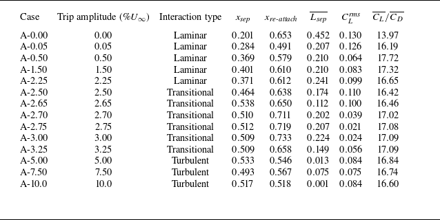


 Cf
 T=5×10⁻⁴
 Cf


 St=1.9


 St=0.08
 St=0.6
 St=1.9

 u
 y=0.003c


 xs
 Tb

 Mr
 x˙s
 hTE
 Mr
 Tb

 0.4
 urms
 vrms
 wrms

 x/c=0.50,0.55
 0.60
 A−2.75
 A−7.50

 A−7.50
 Δt
 Δt/2
 (a)
 (b)
 (c)

 A−7.50



