

At the start of the fourteenth century, population pressure in England was enormous. For a large part of the population, living conditions were difficult (Campbell Reference Campbell2005: 3–4; Kitsikopoulos Reference Kitsikopoulos2000; Postan and Titow Reference Postan and Titow1959). In the course of the thirteenth century, the population had grown, land prices had risen, and real day wages for casual day and piece-rate workers had fallen (Campbell Reference Campbell2005; Clark Reference Clark2007). The economic boom of the later twelfth and thirteenth centuries had lost its momentum, and profit margins for commercial activities were shrinking (Langdon and Masschaele Reference Langdon and Masschaele2006). Around 1300, real wages of annual and day laborers were much lower than they were at the end of the fourteenth century (Clark Reference Clark2007; Claridge et al. Reference Claridge, Delabastita and Gibbs2023), and the diet of the common people was almost completely plant-based (Dyer Reference Dyer1988; La Poutré Reference La Poutré2015). The population stagnated and must already have reached its medieval peak before it was struck by the Black Death and its subsequent waves of plague (Broadberry et al., Reference Broadberry, Campbell, Klein, Overton and van Leeuwen2015: 20).
There is broad consensus among historians that life must have been hard before the plague (Campbell Reference Campbell2005; Jordan Reference Jordan1996: 8–11; Kershaw Reference Kershaw1973; Kitsikopoulos Reference Kitsikopoulos2000; Postan Reference Postan and Postan1966; Schofield Reference Schofield and Müller2021). While living conditions are well understood, the demographic regime – in particular mortality, nuptiality, and household size – and its relation to living conditions are less clear. Should we, or should we not, expect a so-called Western European marriage pattern (Hajnal Reference Hajnal, Glas and Eversley1965), given the Church’s doctrine in 1234 of marriage being based on mutual consent of both bride and groom (De Moor and Van Zanden Reference De Moor and Van Zanden2010; Van Zanden Reference Van Zanden, Van Zanden, De Moor and Carmichael2019)? As many holdings were quite small, might we expect households to have been really small, or might they have been somewhat larger? What kept the population from growing any further: was it Malthus’ positive check, in the form of high mortality, or was it the preventive check?
As demographic information is extremely scarce for this period, available data are too fragmentary to answer these questions decisively. Therefore, this article attempts to complement this evidence with already existing parametrized demographic models. We examine and model quantitatively nuptiality, marital fertility, and mortality around 1300. By connecting the scarce available data to a broader model, doubts about the reliability of the evidence may be assuaged (Bailey Reference Bailey1996: 9; Goldberg Reference Goldberg1992: 3). The use of broad, parametrized, models is well-established in demography (Coale, Reference Coale1971; Coale and McNeil Reference Coale and McNeil1972; Goldstein and Kenney Reference Goldstein and Kenney2001; Pittenger Reference Pittenger1973; Preston et al. Reference Preston, Heuveline and Guillot2001). As the data are limited, we will use only simple models that contain just a few parameters (La Poutré and Janssen Reference La Poutré and Janssen2021).
Our aim is to construct a picture of the demographic regime that is consistent with the available evidence on nuptiality, marital fertility, mortality, and household size. To test whether these models together create a consistent picture, their interplay will be observed with a simple macrosimulation in which we focus on household size. Although “simulation results differ from, and should not be mistaken for, reality” (Zhao Reference Zhao and Zeng2008: 22), they can be valuable to distinguish between highly relevant mechanisms and those of minor importance. Simulations help to determine whether all highly relevant mechanisms are incorporated in the applied models.
In our case, we first review the existing literature to estimate the mean household size around 1300. Second, we use models on nuptiality, marital fertility, and mortality to design a simulation that creates a picture of the demographic regime in England around 1300. In particular, our simulation predicts the mean household size at that time, and it closely matches the estimated mean household size. Despite the scarcity of data from which our three models are created, this close match gives us confidence that the most relevant mechanisms are indeed incorporated.
We prefer our more straightforward macrosimulation to the existing microsimulations that construct individual histories for the analysis of kinship, such as SOCSIM, MOMSIM, and CAMSIM (Ruggles Reference Ruggles1987: 74–105; Smith and Oeppen Reference Smith, Oeppen, Reher and Schofield1993). In these microsimulations, the model’s author has to invent too many additional hypothetical rules for the model to work (Ruggles Reference Ruggles1987: 79, 102–5).
To construct a picture of the demographic regime around 1300, information on mortality, nuptiality, marital fertility, and household size is required. Unfortunately, this information is very scarce. Parish registers, such as have been used to reconstruct Early Modern English population history (Wrigley and Schofield Reference Wrigley and Schofield1981; Wrigley et al. Reference Wrigley, Davies, Oeppen and Schofield1997), did not exist in England before 1538. Lacking better sources, information on demographic variables around 1300 can sometimes be extracted by family reconstitution from court rolls, from manorial lists of tenants, or from Inquisitions Post Mortem. Notably, the Toronto School has put much effort into family reconstitution for medieval England (for an overview, see: Brezette DeWindt Reference Brezette DeWindt and Brettezette DeWindt1995; Razi Reference Razi1979). However, while their studies provided valuable insights into everyday life in village communities, these studies did not concentrate on the quantitative information necessary for our models. Such information is mostly fragmentary and it often requires bold assumptions to convert this information into values for age at marriage, mortality risks, and household size.
No more than a handful of studies, and dealing only with small groups, have done so: Russell’s (Reference Russell1948: 92–117) study of tenants-in-chief, the study of Postan and Titow (Reference Postan and Titow1959) on heriots at five manors of the Bishop of Winchester, Razi’s (Reference Razi1980) study of peasants in Halesowen, Worchester, Hallam’s (Reference Hallam1985) study of peasants in five Lincolnshire’s manors, and Ecclestone’s (Reference Ecclestone1999) study of landless men on two Warwickshire manors are all that we have. We will discuss the underlying assumptions and will re-examine the results of these studies. In addition, Cummins’ (2017) paper on the lifespans of the European elite 800–1800 provides some insight into differences between the common people and the elite.
Abstracting from regional differences, we aim to present a coherent view for England as a whole around 1300. As the lion’s share of the English population lived in rural areas (Campbell Reference Campbell2008: 908–9), we will ignore urban patterns completely.
Migration, while highly relevant between towns and villages and even between regions within the country, was of only minor importance between countries at the turn of the fourteenth century (Schofield and Whittle Reference Schofield, Whittle, Vanhaute, Devos and Lambrecht2011: 51). Immigration through Viking raids and the establishment of subsequent settlements belonged to the past, and emigration to colonies in the Americas was still far in the future. Although England was not isolated from Wales, Scotland, Ireland, or the Continent, migration between these countries was quantitatively only modest in 1300. As quantitative information is not available, the so-called alien subsidy of 1440, which was a poll tax, might give some indication. The alien-born working population at that time could hardly have represented one percent of the population (Thrupp Reference Thrupp1957: 266). As our analysis concentrates on the main aspects of what was going on, migration between countries is left out of the equation.
Demographic information on the elite is more detailed than information on common people, so this article starts with the elite’s mean age at inheriting property and its mortality pattern. This information is used as a reference in the subsequent sections on marital fertility, nuptiality, mortality, and mean household size among common people. To be specific, in Section 2, a simple model on marital fertility is presented. Section 3 concentrates on nuptiality patterns with a discussion of the mean age at first marriage, and the mean age at which peasants first acquired property. Section 4 analyzes mortality patterns for peasants and landless men by estimating their life expectancy and compares it to the elite mortality pattern of Section 1.
Section 5 focuses on the mean household size. Section 6 presents a simple macrosimulation to test the consistency of the constructed models on marital fertility, nuptiality, and mortality, by estimating the mean household size for pre-plague England. In Section 7, the results of this study are discussed.
Elite: age at inheritance and age at death
Medieval documents hardly ever registered when someone was born or baptized, which makes it extremely difficult to determine someone’s age at death. An exception is the Inquisitions Post Mortem that Russell (Reference Russell1948: 92–117) used to assemble data on the elite, which makes his dataset highly relevant to our study. When a tenant-in-chief (a vassal who held his fief directly from the king) died, royal officials drew up such a document to inventory the vassal’s properties. Moreover, the vassal’s date at death and the age of his heir(s) were noted. In many cases, Inquisitions Post Mortem were accompanied by several sworn statements of the heir’s age, linking the heir’s birth to some personal event (Russell Reference Russell1948: 102). The information in these Inquisitions Post Mortem formed the base for customary payments, or for guardianship if an heir was under age (Russell Reference Russell1948: 94). Because of the financial consequences, the Crown was keen to have such a document made up soon after the death of his vassal. Therefore, Russell’s data reliably reflect the mortality pattern of England’s elite. To be more precise, his data reflect the pattern for England’s male elite, since the lion’s share of these heirs were males as a consequence of the custom of primogeniture.
We concentrate on Russell’s data for 532 tenants-in-chief who were born before 1276, because it is his only dataset that was not distorted by plague mortality. As his data did not provide any trustworthy values for the young, Russell (Reference Russell1948: 212–4) suggested “until better estimates are made” to use mortality probabilities for infants and children that were based on death rates in modern India. Ohlin (Reference Ohlin and Floud1974: 61), criticizing “such curious elements of speculation and guesswork,” warned against uncritical, mindless use of Russell’s figures. Taking this into account, we will not use Russell’s suggestions on infant and child mortality, but restrict our analysis to his data for the mentioned 532 tenants-in-chief. From Russell’s (Reference Russell1948: 202) data, the mean age at which these heirs inherited their fiefs can be calculated to have been 27.
Using life tables, Russell (Reference Russell1948: 186) himself calculated the remaining life expectancy at age 20 to have been 29 years around 1300, which implies that the mean age at death for a male member of the English elite reaching age 20 must have been 49 years. Cummins (2017: 426), analyzing his dataset of members of the European elite reaching age 20, calculated the mean age at death to have been about 47 years c. 1300. As we focus on England, we will use Russell’s data, but we should be aware that the remaining life expectancy might be somewhat too high.
As mortality data below age 15 are missing, and Russell’s mortality pattern is somewhat irregular due to the sample size, this pattern can be smoothened and completed by using a simple robust mortality model. The Princeton Model life tables might have served this purpose (Poos Reference Poos1985: 526) if they had not been based on late nineteenth and early twentieth-century life tables alone (Ecclestone, Reference Ecclestone1999: 21–2; Hatcher Reference Hatcher1986: 31; Wrigley et al., Reference Wrigley, Davies, Oeppen and Schofield1997: 263). Instead, the two-parameter model on survivorship that was developed by La Poutré and Janssen (Reference La Poutré and Janssen2021) is a better option as it is empirically founded in demographic material reaching back as far as the seventeenth century, and is found to be flexible enough to adequately fit English mortality patterns from the seventeenth century to today. Before 1850, survivorship
 ${l_x}$
, which is the number of newborns to survive to a certain age
 $x$
, is therefore modeled as a function of the cumulative hazard of mortality
 ${{\rm{\Lambda }}_x}$
, containing only two parameters:
 $${l_x} = C \cdot {e^{\; - {{\rm{\Lambda }}_x}}}$$
with
 $$\Lambda_{x} = {\left({x + 1.5} \right)^{ - 1.7} \over { - 1.7}} + e^\theta \cdot \left( {x + Ln\left( {1 + {e^{\left( {x - 16} \right)}}} \right)} \right) + {{\rm ln \left({1 + e^{\beta \cdot ( x - 100})} \right)} \over{\beta}}$$
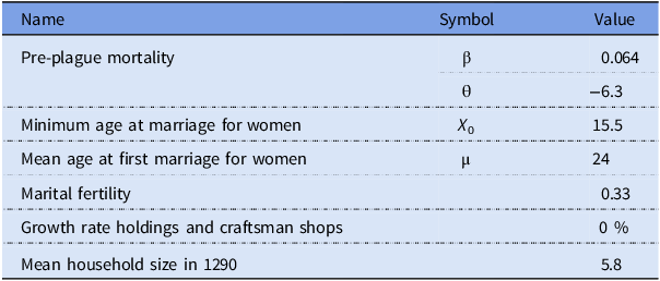
La Poutré and Janssen (Reference La Poutré and Janssen2021) have calculated the best fit to Russell’s data to be at 0.064 for parameter β, representing the rate of aging, and –6.3 for parameter θ, representing the level of mortality risks that are independent of age for adults above age 20. It should be noted that constant
 $C$
is not an independent parameter of this model. It simply guarantees that
 ${l_0} = 1$
.
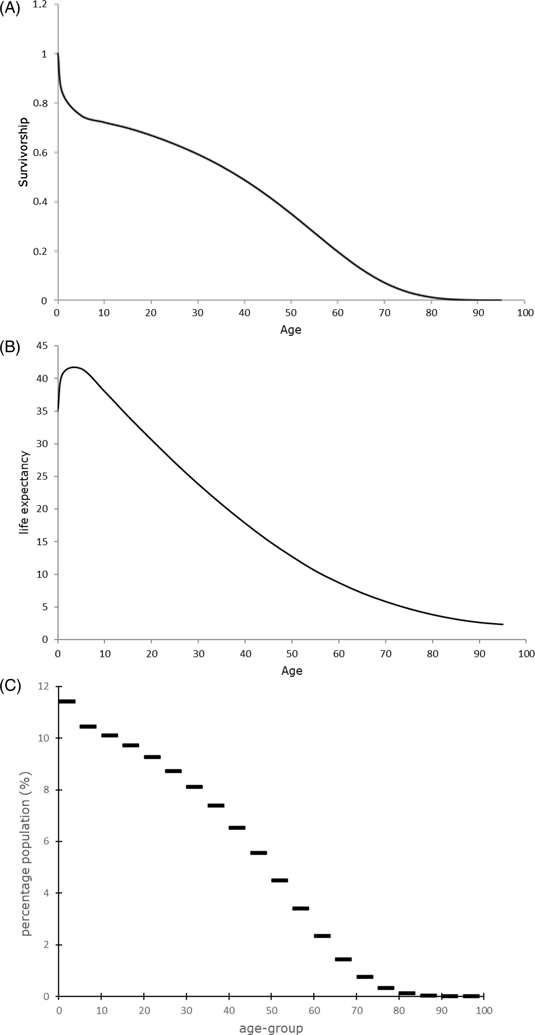
As we expect the population to have been more or less static at its medieval peak, we do not have to differentiate between cohort and period life tables to calculate the corresponding age distribution and life expectancy (see Fig. 1). Furthermore, the crude death rate implied by the survivorship model of La Poutré and Janssen (Reference La Poutré and Janssen2021) can be calculated to have been 0.028 for the elite, which is only slightly above Wrigley et al. (Reference Wrigley, Davies, Oeppen and Schofield1997: 614) results for the sixteenth, seventeenth, and eighteenth centuries, being 0.026, 0.027, and 0.027, respectively.
English tenants-in-chief born before 1276 (n=532). (A) Survivorship at age x of the elite. (B) Life expectancy of the elite. (C) Age distribution of the elite (static population).
Source: La Poutré (Reference La Poutré2023: 61).
Note: Best fit of mortality model (1) at β=0.064 and θ = −6.3. Data age groups 0–4, 5–9, 10–4, 15–9, 20–4, 25–9, ….

As was mentioned earlier, we have calculated the mean age at which these tenants-in chief inherited their fief to have been 27 years. The survivorship model of La Poutré and Janssen (Reference La Poutré and Janssen2021) implies that the remaining life expectancy at age 27 was 26 years (Fig. 1B).
Although the results of this section relate to only a very small part of society, they will be used as a reference in the next sections. We will make plausible that lower-class mortality and the age at which lower-class men inherited must have been about the same as it was for the elite, which makes the results of this section useful for our macrosimulation.
Marital fertility
Before discussing lower-class mortality and nuptiality, however, we explore the third element of our macrosimulation, which describes how the population expanded. Although fertility outside marriage occurred, we assume it to have been quite modest, of no more than a few percent, as it was in Early Modern England (Wrigley et al. Reference Wrigley, Davies, Oeppen and Schofield1997: 219). Therefore, we restrict this discussion to fertility within marriage – i.e., marital fertility, and examine the mean number of births per family per year.
Unfortunately, hardly any quantitative data on marital fertility is available for the fourteenth century. We are therefore forced to rely on information from later centuries.
In their impressive study on English parish registers between 1580 and 1837, Wrigley et al. (Reference Wrigley, Davies, Oeppen and Schofield1997: 396) confirmed Pittenger’s (Reference Pittenger1973) suggestion that the proportion of females being sterile at age
 $x$
, denoted as
 $S{F_x}$
, is exponentially increasing with age
 $x$
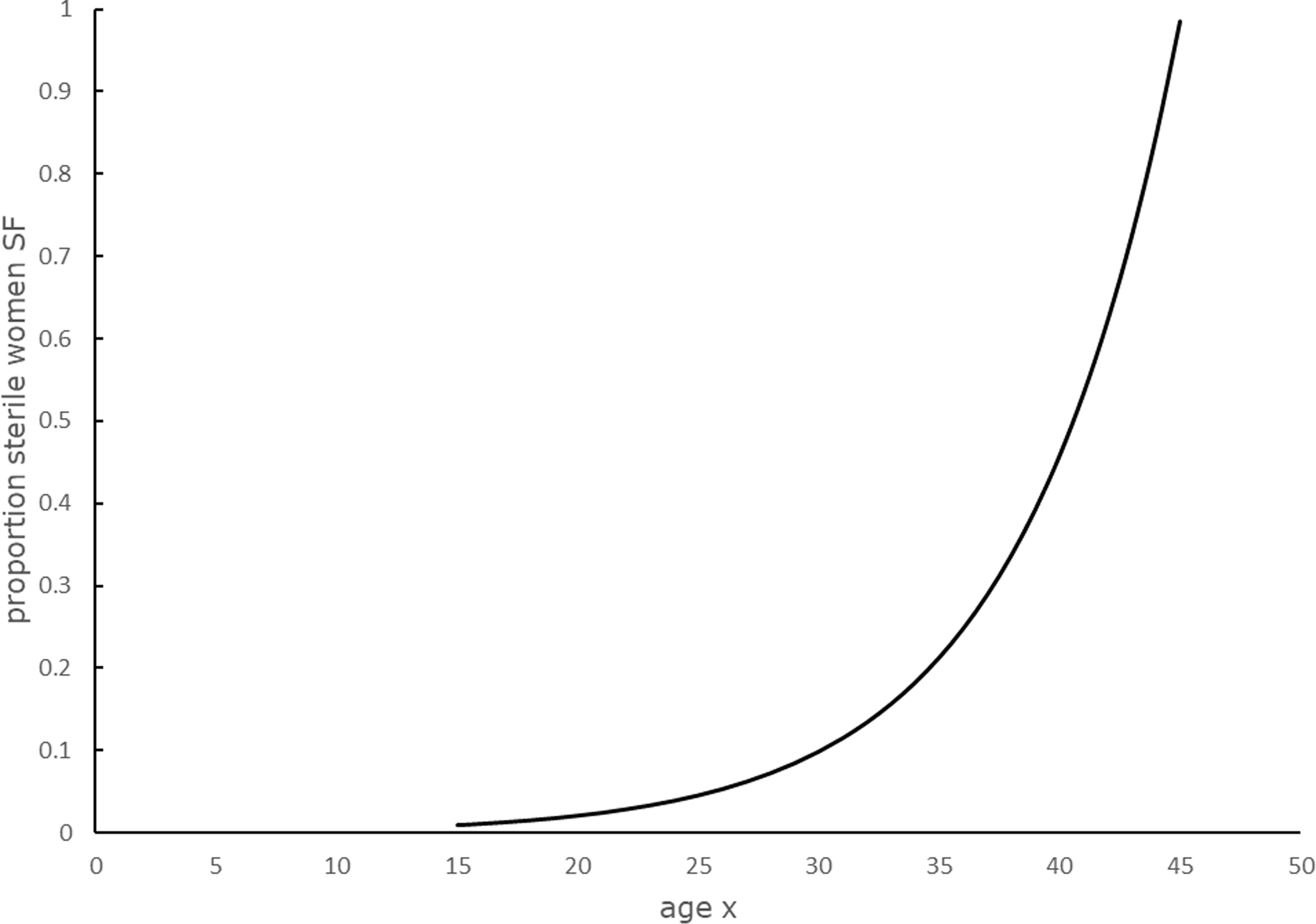
between ages 15 and 45. In formula-form, their result can be written as
 $$S{F_x} = {e^{0.153\cdot x - 6.9}}$$
with age
 $x$
between 15 and 45. Formula (2) is presented graphically in Fig. 2.

This exponential relationship is in line with Clark’s (Reference Clark1977: 10–20) review of twentieth-century data that most women become infertile between ages 40 and 45. Following Smith and Oeppen (Reference Smith, Oeppen, Reher and Schofield1993: 287–8), who used exponentially increasing sterility in their microsimulation model CAMSIM, we will use formula (2) in our macrosimulations in Section 6.
Apart from infertility, marital fertility is also determined by birth interval – i.e., the time between two births, denoted as BI. Although birth intervals are influenced by the mother’s age – complications more often occur in the case of pregnant women below age 20 or above age 35 – we lack the necessary information to take account of this variation in the medieval case. The same applies to the option of a shorter birth interval after the death of the youngest child (Kok et al. Reference Kok, Vandezande and Mandemakers2011: 83). We are forced to assume that the birth interval was the same for all fertile married women.
The aforementioned study of English parish registers between 1580 and 1837 by Wrigley et al. (Reference Wrigley, Davies, Oeppen and Schofield1997: 448) shows that this birth interval decreased from some 32–33 months in the seventeenth century to about 30–31 months at the start of the nineteenth century. Clark (Reference Clark1977: 9–11) gives values for the number of births per year of marriage for several countries in the 1950s, with most of them between 0.37 and 0.43 for young women. Since only a small proportion of these women must have been infertile, these figures correspond to birth intervals of about 28–32 months. As the range for the 1950s is quite close to the one found for Early Modern England, we feel confident to assume that the birth interval was about the same around 1300.
In Section 6, the infertility pattern (formula 2), and the birth interval within the 30–33 months range are used in our simulation to calculate marital fertility.
Age at first marriage, age at first acquiring property
Ever since the mid-twelfth century, the Church propagated marriage should be based on mutual consent of the spouses (De Moor and Van Zanden Reference De Moor and Van Zanden2010; Van Zanden Reference Van Zanden, Van Zanden, De Moor and Carmichael2019). Contrary to parental control in the case of arranged marriages, mutual consent puts groom and bride in control. Before getting married, they often left their parental home to work as apprentices or live-in servants in someone else’s household (Hajnal Reference Hajnal, Glas and Eversley1965: 132; Homans Reference Homans1941: 133–59; Van Zanden Reference Van Zanden, Van Zanden, De Moor and Carmichael2019; Schofield and Whittle Reference Schofield, Whittle, Vanhaute, Devos and Lambrecht2011: 53, Whittle Reference Whittle2017).
There is broad consensus among historians (Devos et al. Reference Devos, Lambrecht, Vanhaute, Vanhaute, Devos and Lambrecht2011: 3; Hajnal Reference Hajnal, Glas and Eversley1965: 133; Homans Reference Homans1941: 144–59; McCarthy Reference McCarthy2004: 51; Razi Reference Razi1980: 66; Schofield and Whittle: Reference Schofield, Whittle, Vanhaute, Devos and Lambrecht2011: 52) that marriage around 1300 was largely restricted to those men who could secure their own economic basis, such as a holding or crafts workshop. However, even casual day and piece-rate workers were usually smallholders with common rights over wastes and pastures and occupied a niche (Bailey Reference Bailey1996:14). Without such a (small-) holding or craft workshop, one could not support one’s family, and marriage was therefore not an option, since nuclear households were largely the norm (Devroey and Nissen-Jaubert Reference Devroey, Nissen-Jaubert, Vanhaute, Devos and Lambrecht2011: 20–2; Hallam Reference Hallam1958: 352). The result was that someone who obtained his own holding or craftsman shop would often marry shortly afterwards – not least because of the Church increasingly condemning sex outside marriage in the course of the twelfth century (Crouch Reference Crouch2017: 235–8).
However, even if this was customary, there must have been many exceptions to this rule. Therefore, it is somewhat risky to equate age at first marriage to age at first acquiring property. Unfortunately, direct information on these two events is so scarce for the medieval period that, without this assumption, it is hardly possible to make estimations for either one of them. For men, it is therefore assumed in this study that these two events occurred simultaneously, and we will jointly discuss the three studies that have examined the age at acquiring first property (Ecclestone Reference Ecclestone1999; Razi Reference Razi1980) or age at first marriage (Hallam Reference Hallam1985). Regrettably, more recent quantitative work on thirteenth and fourteenth-century English nuptiality has not been done yet.
Ecclestone (Reference Ecclestone1999) has studied lists of names, belonging to so-called garciones – most probably landless men (see Appendix A in Supplementary Material) – in court rolls of the manors of Glastonbury Abbey in the late thirteenth and the fourteenth centuries. As these names in subsequent years were explicitly given in the same order, individual garciones can be followed on an annual basis. From his study, the mean age at first marriage can be shown to have been 27 years (see Appendix A in Supplementary Material).
Razi (Reference Razi1980: 10, 84), studying Halesowen (Worcestershire), has reconstructed three generations of 285 families from manorial court rolls within the period 1280–1349. In Appendix B in Supplementary Material, we argue that his findings suggest that the mean age at first marriage for men was probably 25 years.
In contrast to what Clark et al. (Reference Clark, Cummins and Curtis2024: 2) found for early nineteenth-century England, however, Razi’s study suggests that at the start of the fourteenth century, the offspring of well-to-do families probably married significantly younger than those of poorer families. Razi (Reference Razi1980: 43–60) describes some cases of several richer families who were able to provide their sons with some land while their father was still alive. Furthermore, the remaining life expectancy at age at first marriage was much lower, i.e., no more than 21 years, for the poorer part (smallholders and cottagers) of Halesowen than for the richer part (customary tenants of half virgates and virgates) – i.e., 33 years. Although his results might suggest that smallholders and cottagers died rather young compared to their richer community members, our discussion on mortality in the next section suggests that these differences were rather small. Therefore, it seems more plausible that the sons of poorer families married rather late.
Hallam (Reference Hallam1985) has estimated the age at first marriage and the age at death at five manors in Lincolnshire in the Late Middle Ages, by studying merchets, which are licences for customary tenants to marry off their daughters (Razi Reference Razi1980: 45). At these manors, merchets often gave the names of both bride and groom. Our re-analysis of his results shows that the mean age at first marriage must have been about 24 years for women and within the range 26–35 for men (see Appendix C in Supplementary Material).
Taken together, the three studies suggest that around 1300 the mean male age at first marriage of the common people was somewhere in the range 26–29, which is close to the mean age at which the elite tenants-in-chief had inherited their fief such as we saw in the previous section – i.e., age 27. What is more, it is even in line with the mean wedding age for men in the seventeenth and eighteenth centuries (Hallam Reference Hallam1985: 59). All in all, this marriage pattern seems to have been remarkably stable. Furthermore, the (mean) age difference between the spouses is fairly small, as might be expected when marriages were based on mutual consent (De Moor and Van Zanden Reference De Moor and Van Zanden2010; Van Zanden Reference Van Zanden, Van Zanden, De Moor and Carmichael2019).
From Hallam’s (Reference Hallam1985) study, the age distribution of female first weddings can be established with the use of a well-established demographic model. In 1971, Coale observed that age distributions of female first weddings showed much similarity for a wide range of societies. Coale and McNeil (Reference Coale and McNeil1972), and Coale and Trussell (Reference Coale and Trussell1974), further exploring this observation, proposed the so-called Coale-McNeil model, containing 3 parameters, to describe the proportion of females that gets married for the first time at age
 $x$
, denoted as
 ${W_x}$
:
 $${W_x} = C \cdot \;{e^{ -\, {{{0.174}} \over {K}} \ \left( {x - {x_0} - 6.06K} \right) \ - \ {e^{ -\, {{{{{0.2881}}\over {K}}}}\ \left( {x - {x_0} - 6.06K} \right)}}}}\;\;\;$$
in which
 $x$
represents the woman’s age, and parameter
 ${x_0}$
the minimum wedding age. Parameter K is a scale factor (in years) that reflects the spread of this distribution of female first weddings, and the value of parameter C is determined by the proportion eventually married. Furthermore, the mean age at first wedding, denoted by µ, can be expressed in terms of two parameters of this model (Preston et al. Reference Preston, Heuveline and Guillot2001: 203):
 $$ \mu = {x_0} + 11.36 \cdot K$$
Ever since, this nuptiality model is well-established among demographers (Preston et al. Reference Preston, Heuveline and Guillot2001: 202–4). What is more, equation (3) cannot only be shown to fit nineteenth and twentieth-century age distributions well (Coale Reference Coale1971; Goldstein and Kenney Reference Goldstein and Kenney2001) but also those in England during the entire period between 1600 and 1837 as established by Wrigley et al. (Reference Wrigley, Davies, Oeppen and Schofield1997: 146–7). Furthermore, when the best fit of equation (3) is calculated for the English age distributions of female first weddings for the period 1600–1837, minimum age parameter
 ${x_0}$
appears to have been about age 15.5 throughout this long period. This value is consistent with the observation by Wrigley et al. that only in less than 1 percent of all first marriages, brides were younger than 16 years old.
Probably, this minimum age also applied to the fourteenth century. Although the canonical age was 12 (Hallam Reference Hallam1985: 57), it seems most plausible that a girl only married below the age of 16 in exceptional cases. For instance, to secure inheritance, “elite girls of fourteen or fifteen could be deemed of sufficient emotional maturity to enter marriage without long delay” (Philips Reference Philips2003: 33). In such cases, there seems to have been a tendency to postpone consummation of marriage (Philips Reference Philips2003: 36, 39).
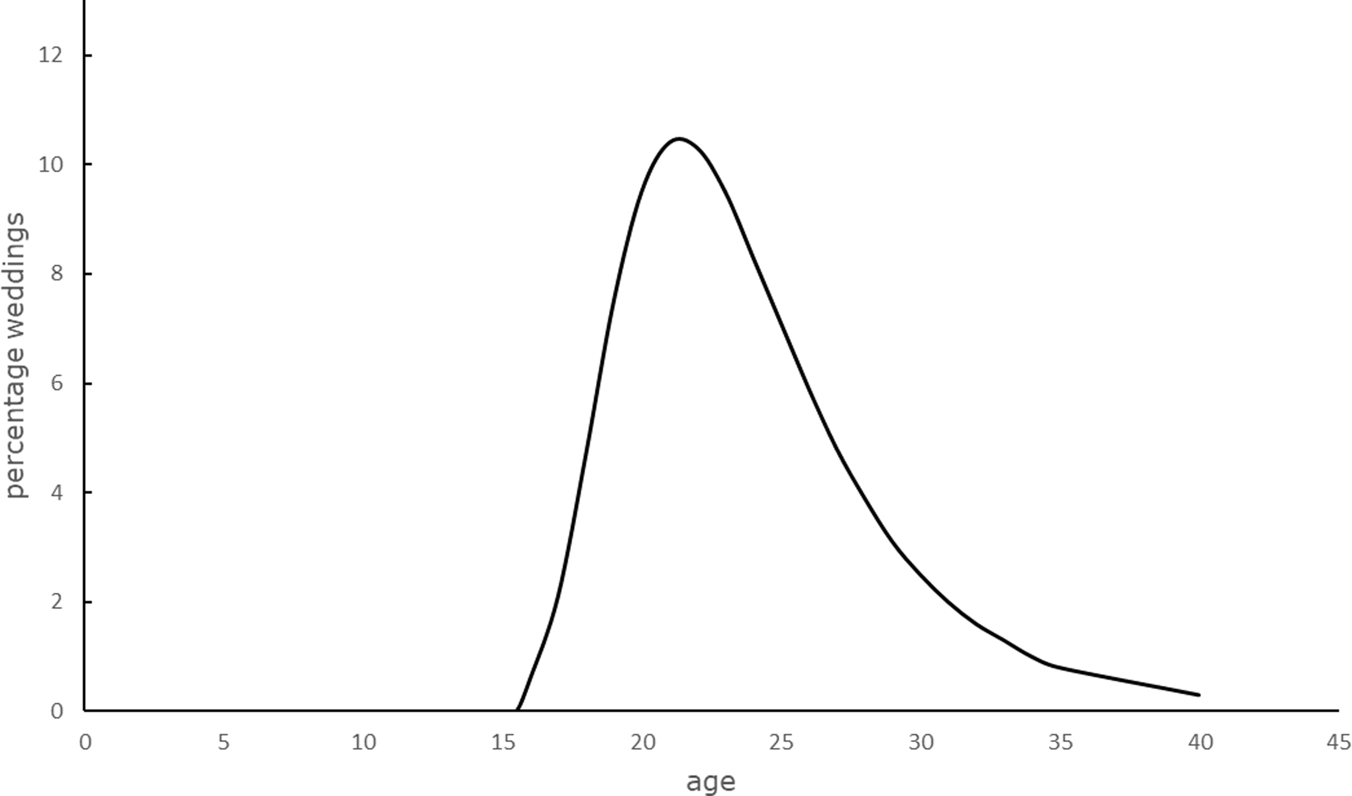
As was already explained earlier, we have corrected Hallam’s estimate for the female mean age at wedding to 24. This result, combined with the minimum age of 15.5, can be used to calculate scale factor K from equation (4) to have been 0.75 years. The corresponding age distribution for female first weddings c. 1300 is given in Fig. 3.

Following Smith and Oeppen (Reference Smith, Oeppen, Reher and Schofield1993: 287), who used the Coale-McNeil model in their microsimulation model CAMSIM, we will use this distribution in our macrosimulation in Section 6.
Lower-class mortality
Elite mortality has already been analyzed in Section 1. In this section, we now estimate death rates and life expectancy for the common people and compare these results to the mortality pattern for the elite.
A few scholars have studied mortality of common people in the pre-plague period: Postan and Titow (Reference Postan and Titow1959) studied five manors of the Bishop of Winchester; Ohlin (Reference Ohlin and Floud1974) evaluated their study; Razi (Reference Razi1980) studied peasants in Halesowen, Worcestershire; Hallam (Reference Hallam1985) examined five manors in Lincolnshire Fenland; finally, Ecclestone (Reference Ecclestone1999) focused on two manors in Warwickshire. In all five studies, surviving court rolls provided the necessary data. While Postan and Titow simply counted death duties, Hallam, Ecclestone, and Razi estimated life expectancy and death rates from family reconstitution data. It should be noted that these last three studies were already introduced in the previous section, as Hallam, Ecclestone, and Razi did not concentrate on mortality alone but studied nuptiality or the acquisition of property as well.
Postan and Titow (Reference Postan and Titow1959) studied heriots, which were death duties, for five manors of the Bishop of Winchester’s estate between 1245 and 1349: Taunton, Meon, Waltham, Wargrave, and Fareham. Most often, such duties were levied on holdings of customary tenants soon after the death of the landholder. Heriots were usually paid in the form of animals, but money payments occurred as well. Postan and Titow (Reference Postan and Titow1959) restricted their study to the mentioned five manors because both animal and money heriots were registered in the bailiffs’ accounts of these manors.
Their data suggest that the remaining life expectancy at the mean age to take up land was within the range 19–25 years (La Poutré Reference La Poutré2023: 80–1, 91; Ohlin Reference Ohlin and Floud1974).
The Halesowen manorial court rolls registered the death of 250 male tenants between 1300 and 1349, “when the heir of the deceased paid heriot and an entry fine or when he was taken into custody, or when the holding escheated for default of heirs or for failure to pay the customary fines” (Razi Reference Razi1980: 34). Of these tenants, 196 were well-documented. For them, Razi (Reference Razi1980: 43–5) calculated that the mean interval between their first appearance as landholder and their year of death was 30 years. Among these 196 men, only 49 of them – being cottagers and smallholders – belonged to the poorer part of the village, which is only 25 percent instead of the 43 percent it should have been if this poorer part was represented properly (Razi Reference Razi1980: 43). Because their mean interval was much lower – i.e., only 21 years – Razi (Reference Razi1980: 43–4) added 62 fictitious poor tenants, thereby correcting his result to 28 years. Arguing that those tenants that he had missed in the court rolls might even have belonged to the poorest part of society, maybe dying even younger, he suggested an interval between 25 and 28 years.
The third study on peasant mortality is Hallam’s (Reference Hallam1985) study on five Lincolnshire manors in the Late Middle Ages. Gathering records of merchets – licences for customary tenants to marry off their daughters – from a sacrist’s register compiled from court rolls, he has analyzed 90 women who were married twice, assuming that these widows remarried within a year after the death of their husband. He estimated the mean age at death for these men to have been 51, by assuming that “at marriage before the Black Death men were 26,” and by calculating the years between the women’s first and second marriage (Hallam Reference Hallam1985: 63). Actually, he thus calculated the remaining life expectancy at first marriage to have been 25 years.Footnote 1
Hallam himself expected this calculation to have produced an age at death above the real value, because of his assumption of remarriage within a year. However, it seems quite plausible that there was a bias towards the younger widows remarrying, which would result in an estimated age at death below the real value.
Hallam also suggested a second method which is, however, far too inaccurate to be considered here (La Poutré Reference La Poutré2023: 83–6).
The fourth study on lower-class mortality is by Ecclestone (Reference Ecclestone1999). As was noted above, he studied head-tax lists for garciones on the manors of Longbridge Deverill and Monkton Deverill (Warwickshire) between 1295 and 1350. Concentrating on the ones he had identified as sons of residential families, he was able to establish for 279 garciones at what age they entered tenure, left the manor, or died. For only 46 of them, he could actually establish their age at death, because the others disappeared from sight when they acquired land or left the manor (see Appendix A in Supplementary Material).
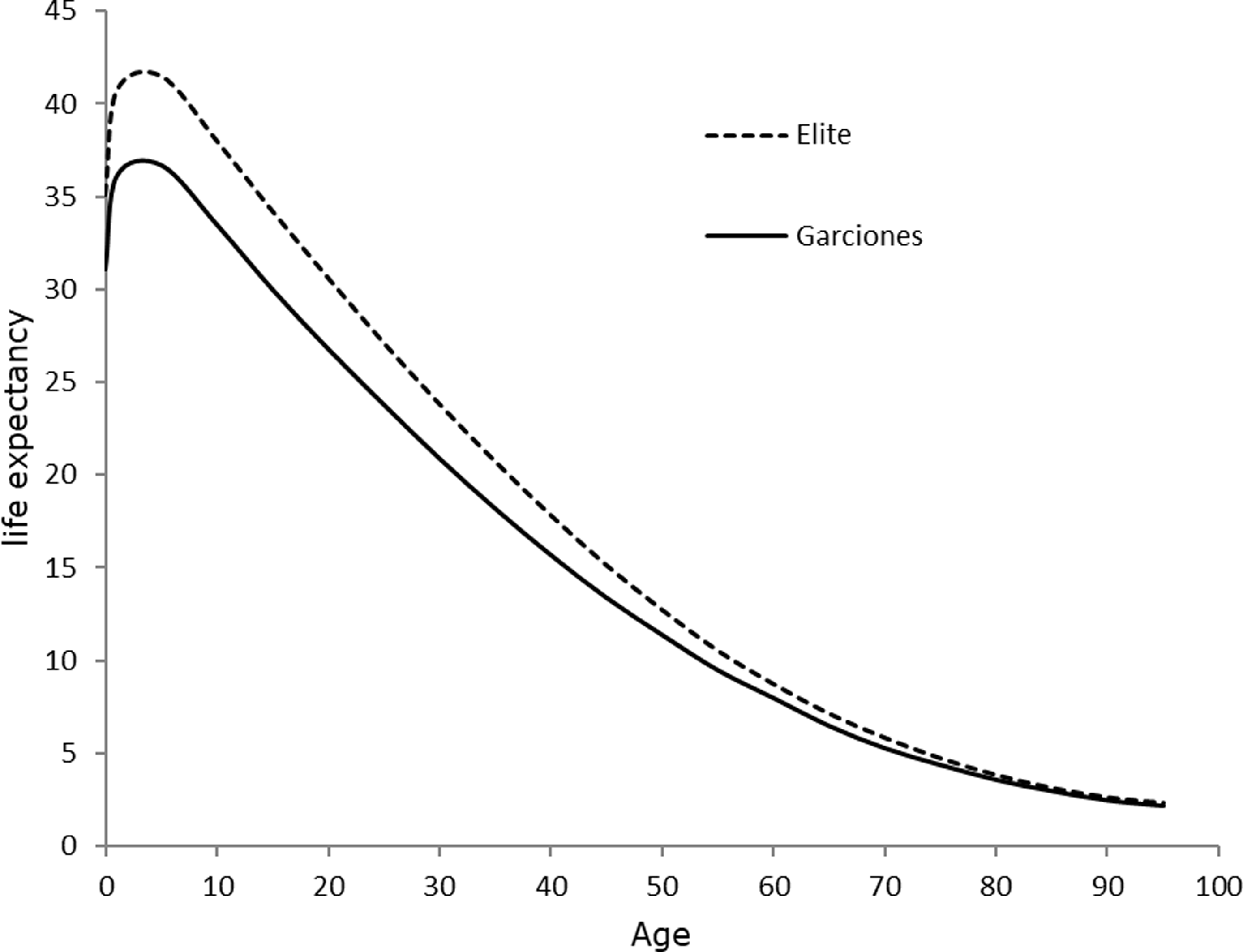
The mortality pattern for these garciones can be compared to the one for the elite, as already described before. In Fig. 4, life expectancy of garciones, being landless men, and of tenants-in-chief, who were members of the elite, is shown in one figure. The difference in the remaining life expectancy rose to 4.5 years in childhood but became smaller in adulthood. Given the large error of fit for garciones, the differences for adult men were quite moderate.

Despite their small datasets and their diverging methods to obtain their data, the four studies on rural male mortality present a fairly similar picture of male mortality. Three of them estimate the remaining life expectancy at the mean male age to acquire land, or to marry, which we have already established to have been about age 27. Ohlin estimates the remaining life expectancy at acquiring land at five manors of the Bishop of Winchester to have been some 19–25 years. Razi estimates it to have been some 25–28 years at Halesowen, Worcestershire. Hallam estimates the remaining life expectancy at marriage at five manors in Lincolnshire to have been some 25 years. Furthermore, Fig. 4 shows the remaining life expectancy at age 27 to have been 23 years for landless men at two manors of Glastonbury Abbey.
The mean value for these four remaining life expectancies at first marriage or at acquiring land is 24 years (22 years for the Bishop of Winchester’s estate, 26.5 years for Halesowen, 25 years for Lincolnshire’s Fenland, 23 years for garciones of Glastonbury Abbey), which is two years below what we found for the elite in Section 1. However, whether the elite’s more favorable living conditions were only partly balanced by the substantial risk to die in battle, and the intake of vast quantities of alcohol (Cummins 2017: 426, 434), cannot be concluded from this study. Given the small size of the datasets, one should not put too much confidence in the magnitude of this difference.
That being said, it is in line with Clark’s (Reference Clark2007: 97–98) observation of only a modest effect of income on life expectancy in early seventeenth-century England.
Household size
Given the similarity between life expectancy of landless men, peasants, and the elite, we will use the mortality pattern for the elite to make a well-underpinned estimation of the mean household size around 1300. According to Fig. 1C, 68.5 percent of the population was above age 13. Postan (Reference Postan and Postan1966: 619–20) has calculated the number of customary tenants, of whom the lion’s share was male, on 32 manors of Glastonbury Abbey to have been 2,046 in the mid-thirteenth century. More than half of them, as much as 1,094, were smallholders, holding no more than a quarter virgate or even less, but they all were probably heads of households. Ecclestone counted the names on lists of garciones, identified as landless sons of villeins of age 14 or older (Fox Reference Fox, Razi and Smith1996: 518–38), on these same manors to have been 2,200 in 1307–8 (Ecclestone Reference Ecclestone1999:14). As even casual day and piece-rate workers were usually smallholders with common rights over wastes and pastures (Bailey Reference Bailey1996: 14), these landless men rarely had a household of their own. Instead, they lived, unmarried, in someone else’s household. Given that the names of these garciones were tabulated year after year (see Appendix A in Supplementary Material), we believe that these lists were more or less complete, because it seems implausible to us that large numbers of garciones were able to live unnoticed by the officials for a long period of time.
If the number of customary tenants kept pace with the total population, their numbers would have grown from 2,046 around 1250 to about 2,353 in 1307.Footnote 2 In total, then, customary tenants and their landless sons and brothers would have summed up to 4,553 men. With 68.5 percent of the population above age 13, and half the population being female, these customary households contained 13,293 persons in total. Divided over 2,241 holdings, the mean household size was 5.9.Footnote 3
Such a high figure is not as exceptional for a pre-industrial European rural society as one might think, since it is equal to what has been found for Sweden in the century and a half before 1751 (Palm Reference Palm1999). Nevertheless, it lies some 1.0 above the figure that is widely accepted for thirteenth-century England (Hallam 1958: 340, Reference Hallam1963; Howell Reference Howell1983: 232–5; Razi Reference Razi1980: 83–6, 93; Schofield Reference Schofield2003: 83–4), and it is way above the figure defended by Russell (Reference Russell1962), which was as low as 3.5.
To evaluate the difference between the household size estimated above and the ones in the studies just mentioned, one has to address other available quantitative evidence as well. For the pre-plague period, this evidence is limited to no more than two studies, which are those of Hallam (Reference Hallam1958) and Howell (Reference Howell1983).
The third study often referred to, which is Russell’s (Reference Russell1948: 26–7), is irrelevant, since his data came from the 1377 poll tax and thus relate to the situation shortly after a major plague epidemic had struck the country in 1375. High mortality during the epidemics of 1348–49, 1360–61, 1369, and 1375 caused a shortage of workers (Broadberry et al. Reference Broadberry, Campbell, Klein, Overton and van Leeuwen2015: 83). The impressive rise of real day wages during the second half of the fourteenth century may give an indication of this labor shortage (Clark Reference Clark2007: 99–100). Furthermore, high mortality within households may have reduced the mean household size and may have even wiped out whole households. As rising real wages and vacant holdings must have created many opportunities for unmarried adult servants to get married and start their own family, household composition in 1377 must have seriously deviated from the high population pressure regime around 1300. Therefore, such data cannot be expected to be representative of the pre-plague period (La Poutré Reference La Poutré2023: 265–72).
Hallam (Reference Hallam1958) studied serf lists from the manors of Weston, Moulton, and Spalding, which are three manors of the Spalding Priory on the Lincolnshire Fenland. From his results, we calculate that the mean household size was 5.3 (see Appendix D in Supplementary Material).
Howell (Reference Howell1983: 209–15) has reconstructed the population of Kibworth Harcourt from the 1280 tithing list, which listed all male inhabitants over the age of 12. She counted 48 males over the age of 12 for 21 half virgates (Howell Reference Howell1983: 230). Assuming the number of males and females to have been equal, the mean household size must have been 4.6, only counting members over 12. According to Fig. 1C, concerning the elite, 27 percent of them had been under 12. If we assume that this percentage also applied to peasants, their mean household size was 6.3.
Our discussion of Hallam’s examination of three manors of the Spalding Priory, which results in a mean household size of 5.3, of Howell’s study of Kibworth Harcourt, which leads to a mean household size of 6.3, and our own estimation of the mean household size at 32 manors of Glastonbury Abbey to have been 5.9, comes down to a mean household size of 5.8.
This figure is exactly the same as the one that follows from a theoretical family model that Howell (Reference Howell1983: 221–35) constructed on the basis of her study of the manor of Kibworth Harcourt. She only used the estimated age at first marriage, the remaining life expectancy at marriage, and the assumption that the standard birth interval was 30 months, thus 2.5 years. Her model, which is very instructive, results in four children per married couple to reach age 12, and a mean household size of 4.84 persons aged 5 or over (Howell Reference Howell1983: 233). Including children under age five, as specified in her model, results in a mean household size of 5.8 persons.
Demographic macrosimulation
In the previous sections, we proposed parameterized demographic models for English mortality, nuptiality, and marital fertility around 1300. The values these models’ parameters have taken are based on the few quantitative results that are available in demographic historical studies on pre-plague England. Given the scarcity of medieval demographic material, these few studies cannot be expected to provide a firm empirical basis. However, if it can be shown that these models create a coherent demographic image of English society around 1300 that predicts the mean household size correctly, we may have some confidence in their parameters’ values. To show that the picture is indeed coherent, the three models on mortality, nuptiality, and marital fertility are used in this section to run a macrosimulation for the period 1290–1315. We confine the macrosimulation to this period, because there is broad consensus that the population hardly grew or shrank between 1290 and 1315 (Broadberry et al. Reference Broadberry, Campbell, Klein, Overton and van Leeuwen2015: 12, 15; Clark Reference Clark2007: 120; La Poutré Reference La Poutré2023: 326–30; Poos Reference Poos1985: 521–3). We use demographic projection to check whether the interplay of these three models leads to a stagnating population, as might be expected at the medieval population peak around 1300. In Appendix E in Supplementary Material, the simulation is described in detail. The complete computer source code is given in Appendix F in Supplementary Material.
Besides the models on mortality, nuptiality, and marital fertility, the simulation contains a condition on the number of households. In the late thirteenth and early fourteenth century, new holdings and craft workshops were not easily created, so the number of households could not grow rapidly. Commercial growth slowed down substantially, which may have diminished opportunities for families to make a living (Langdon and Masschaele Reference Langdon and Masschaele2006). It is true that new holdings were created when wasteland was brought under cultivation, but such large projects were quite rare in the first half of the fourteenth century, because only low-quality marginal soils were not yet used for agriculture (Postan Reference Postan and Postan1966: 548–59; Postan & Titow Reference Postan and Titow1959: 410). Occasionally, demesne land was divided to create new half virgates, existing holdings were split, or new cottages were built, but these new holdings and craftsman shops formed no more than a small percentage of the total number of already existing households. As there is broad consensus that the population stagnated between 1290 and 1315 (Broadberry et al. Reference Broadberry, Campbell, Klein, Overton and van Leeuwen2015: 12, 15; Clark Reference Clark2007: 120; La Poutré Reference La Poutré2023: 326–30), we assume that no new holdings and craftsman shops were formed and that the number of households remained the same in the period 1290–1315.
Calculating next year’s age distributions of population and housewives from the year before for 25 consecutive years between 1290 and 1315 makes it possible to simulate demographic trends within this period. Table 1 presents an overview of the seven parameters that control the simulation. For five of these parameters, their value has already been determined in previous sections. Furthermore, the growth rate of holdings and craftsman shops has been assumed to have been zero. As the population did not grow, the mean household size should remain the same during the simulation.
Overview of the simulation’s input parameters

For marital fertility, a parameter that expresses birth interval
 $BI$
and the proportion of widows
 $WW$
is used to link fertile housewives to births per year (see Appendix E in Supplementary Material). With a birth interval of 30–33 months (see Section 2) and a proportion of widows of 8–10 percent (see Appendix D in Supplementary material), this parameter
 $\frac{{1 - WW}}\over{{BI}}$
on marital fertility lies within the 0.33–0.37 range. Its appropriate value can be determined by running the simulation for several values and selecting the one with the most plausible results.
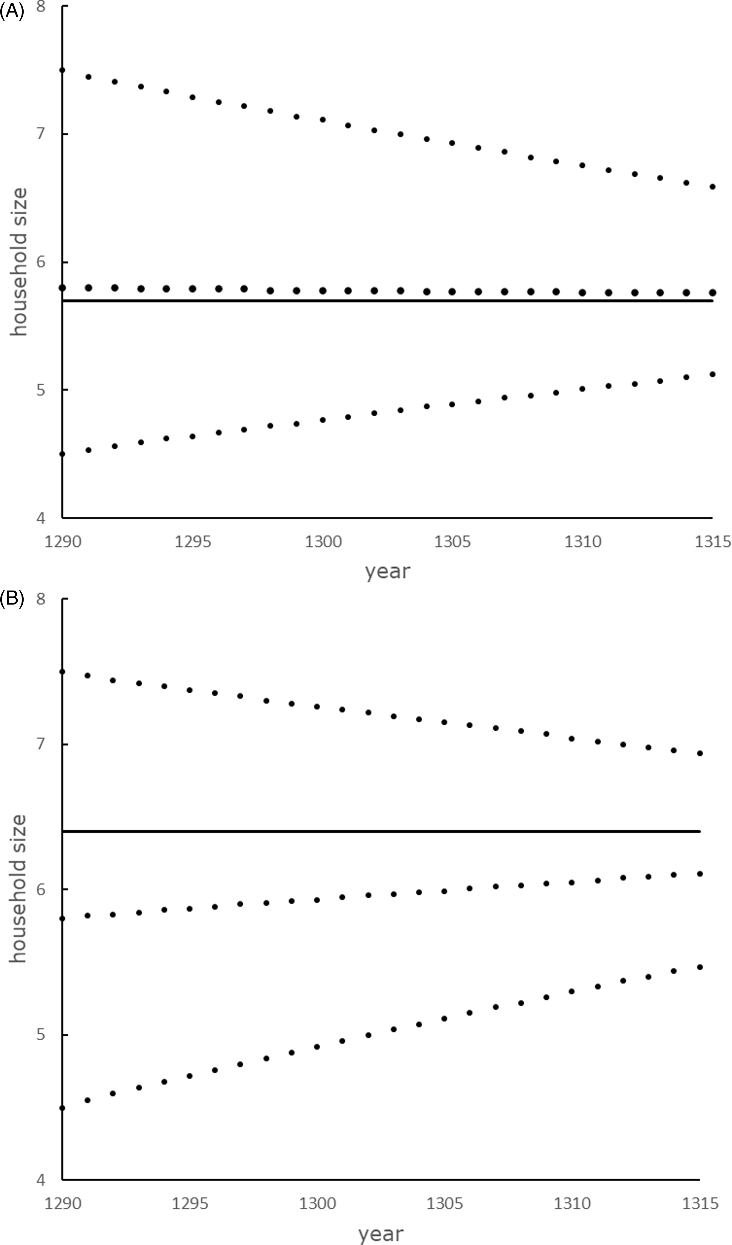
The results of eight simulations, varying mean household size in 1290 and marital fertility only, are presented in Fig. 5. The four time series for which our parameter on marital fertility is taken at its lower bound (0.33) show that the mean household size remains the same if it is set at 5.7 in 1290, which is slightly below the value of 5.8 found in the previous section. If our parameter on marital fertility is taken at its upper bound (0.37), the mean household size does not change if it is set at 6.4 in 1290. Based on these simulations, it seems most likely to take our parameter on marital fertility at its lower bound, which corresponds to circumstances in which 10 percent of all housewives were widows and the birth interval was 33 months.

Thus, our simulation predicts a mean household size of 5.7 members. This result is quite close to the observed value found in the previous section. This close match strengthens confidence that our simulation gives a fair image of the demographic regime around 1300 and that the established values for all seven parameters may be valid.
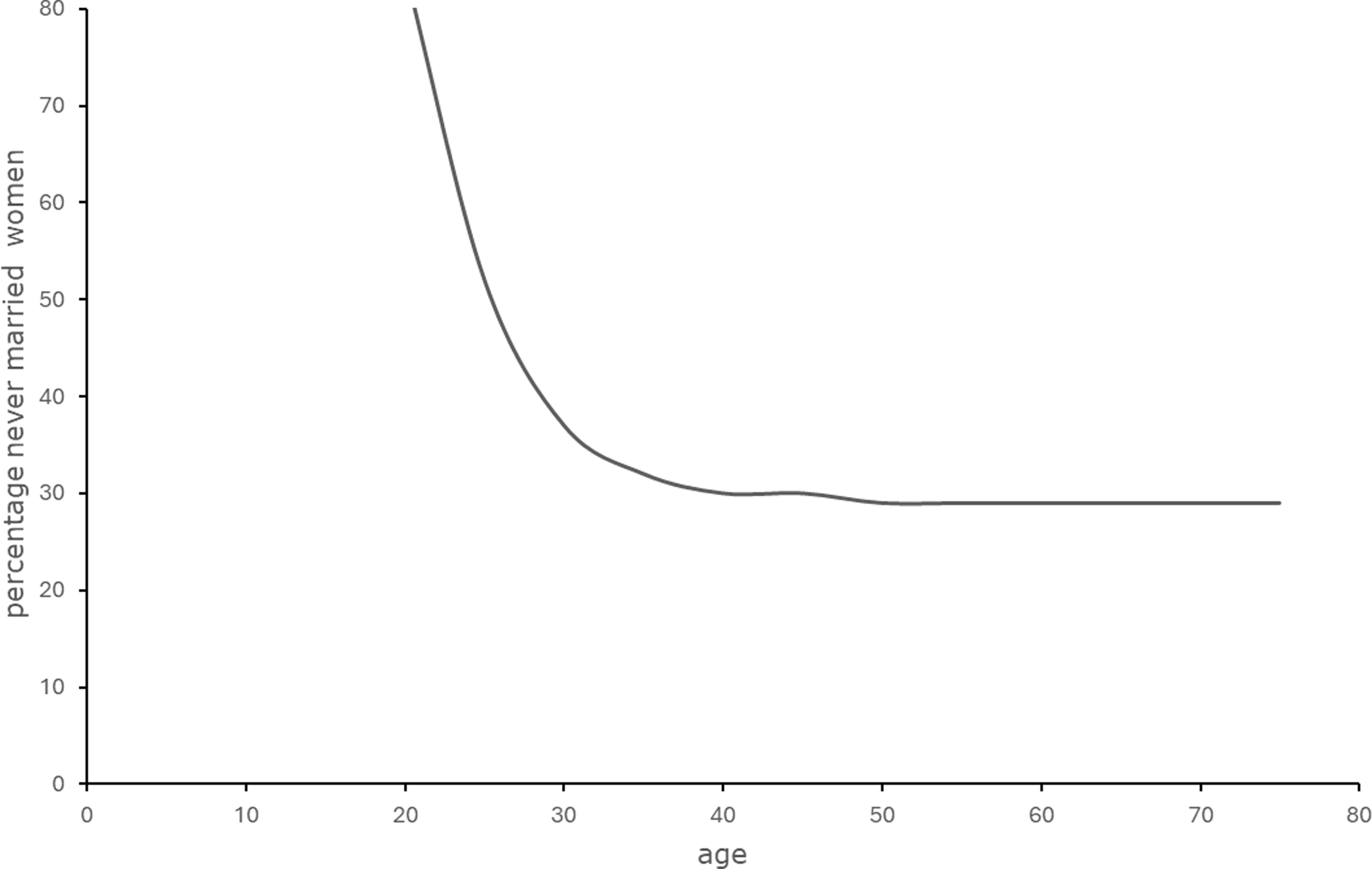
Our simulation also calculates the proportion of women being unmarried. The results are displayed in Fig. 6. As much as 30 percent of the females of age 40 were still unmarried and would remain unmarried for the rest of their lives. They must have lived their lives as unmarried sisters in the household of their brothers or sisters, as nuns, or as live-in servants. This percentage is substantially higher than it was in Early Modern England, when it mostly varied from 10 to 20 percent (Clark et al. Reference Clark, Cummins and Curtis2024; Schofield Reference Schofield1985; Weir Reference Weir1984; Wrigley et al. Reference Wrigley, Davies, Oeppen and Schofield1997: 195).
Percentage never married women in 1290–1315 according to the simulation.
Source: Author computations.
Note: For input parameters, see Table 1.

Many unmarried women and men may have left their parental home. Ecclestone’s (Reference Ecclestone1999: 16, 20) data on garciones show that of 145 boys at age 14, no more than 22 still lived as landless men at their manor of birth when they had reached age 34. While part of these 145 boys must have died or gotten married before age 34, Ecclestone’s figures, combined with our result that about 30 percent of the adults remained unmarried, suggest that more than half of the unmarried brothers must have left their manor of birth.
Discussion
While the family demography of Early Modern England is well-known, the medieval picture is more uncertain. In this article, we have studied nuptiality, marital fertility, mortality, and the mean household size around 1300. With respect to nuptiality, we find hardly any difference between the mean age at first marriage for male peasants and for the elite, which was probably about 27 years for both. For peasant women, the mean age at first marriage was probably about 24 years, which is in line with the Western European Marriage Pattern in the Early Modern Period (Hallam Reference Hallam1985; Van Zanden Reference Van Zanden, Van Zanden, De Moor and Carmichael2019). As might be expected for this pattern, the mean age at first marriage was thus high for both men and women (Bailey Reference Bailey1996), and the age difference between the spouses was quite small compared to Non-Western European marriage patterns.
Furthermore, our analysis suggests that mortality risks for the common people were somewhat higher than for the elite. The remaining life expectancy at age 27 was found to have been about 26 years for the elite, and 24 years for peasants and landless men. Unfortunately, the evidence is too flimsy to be decisive.
That being said, with the remaining life expectancy at marriage somewhat below the mean age at marriage, most parents had already died when a couple got married, or died shortly afterwards. So, according to our findings, three generations under one roof might have been valid for only a small minority of all households c. 1300, which is in line with earlier observations (Hallam Reference Hallam1958: 352; Devroey and Nissen-Jaubert Reference Devroey, Nissen-Jaubert, Vanhaute, Devos and Lambrecht2011: 20–2; Ruggles Reference Ruggles1987: 106–26). Instead, nuclear households, if there were no living-in unmarried brothers and sisters, or laterally extended family households, if there were, must have been the norm. In both options, there might have been living-in servants as well (Hammel and Laslett Reference Hammel and Laslett1974: 87; Howell Reference Howell1983: 228–9). Whether they actually lived under the same roof, or lived in an annexe close to the main house, cannot be determined here.
The mean household size has been found to have been about 5.8. This figure is 15–20 percent higher than what is usually taken for granted for the pre-plague period. Nevertheless, our result is in line with all available empirical evidence and largely in line with a macrosimulation that is based on mortality, nuptiality, and marital fertility as estimated in this study. Taken together, they create a coherent image of English family demography at its medieval peak.
This coherency is a strong indication that the combination of the available scarce medieval data with the applied demographic models in this article gives a reasonable picture of the most relevant aspects of the demographic pattern of this period.
Of course, all household members had to be fed. Especially at the start of the fourteenth century, when the population size was at, or near, its medieval peak, and peasant holdings were relatively small, one might wonder how these farms were able to produce enough food to do so. Based on the output of seigniorial farms, Kitsikopoulos (Reference Kitsikopoulos2000: 248–50) concluded that at least 18 acres of arable land were necessary to sustain a five-member household, but Kanzaka (Reference Kanzaka2002: 599) reported that almost three-quarters of the 30 thousand holdings he had studied were smaller. However, manure flows on peasant farms have shown that peasant land was much better fertilized than seigniorial land, which must have resulted in much higher yields (La Poutré Reference La Poutré2017). Furthermore, these peasant households must have been able to put in much more labor per arable acre, which must have raised peasant yields even further (Hatcher Reference Hatcher2024). Combined with an almost completely plant-based diet (La Poutré Reference La Poutré2015), a farm with 11 acres of arable land must have produced enough cereals, peas, and beans to sustain a family of nearly six persons (La Poutré Reference La Poutré2023: 187–236).
With a mean household size of 5.8, natural fertility rates usually lead to population growth. One might raise the question how this household size could have been consistent with zero population growth. According to us, the answer to this question lies in the high proportion of unmarried adults at the start of the fourteenth century. Economic circumstances prevented many adults from starting a family of their own. As was already mentioned, new holdings and craft workshops were not easily created, and real wages were substantially lower than they were at the end of the fourteenth century (Clark Reference Clark2007; Claridge et al. Reference Claridge, Delabastita and Gibbs2023). Unable to start a family, many adults remained unmarried their whole life. They must have ended up as an unmarried family member in the household of a relative, or as a servant in someone else’s household, as a soldier, a monk, or a nun (Hajnal Reference Hajnal, Glas and Eversley1965: 132).
According to our macrosimulation, about 30 percent of the adult population above age 40 would never marry, which is quite high compared to celibacy in Early Modern England, when, as has been mentioned before, it was mostly within the 10–20 percent range (Schofield Reference Schofield1985; Weir Reference Weir1984: Wrigley et al. Reference Wrigley, Davies, Oeppen and Schofield1997: 195). Nevertheless, the numbers on customary tenants and garciones on 32 manors in Glastonbury Abbey, given in Section 5, indicate that many adults must have remained unmarried. Furthermore, this high percentage of unmarried servants and living-in relatives is consistent with the found large mean household size in a stagnant population. These households were not large because of many children, but because of many singles. As no more than one-third of the household members were children, the population hardly grew. Unfortunately, more specific data to underpin this conclusion have not been discovered yet.
Even those who did end up married often worked as live-in servants when they were still young adults (Schofield and Whittle Reference Schofield, Whittle, Vanhaute, Devos and Lambrecht2011: 53). This enormous reservoir of unmarried men and women, almost completely invisible in medieval sources, seems to have paid the price to keep society away from a Malthusian positive check.
It was the preventive check of late marriages and a high percentage of singles that caused population growth to stagnate. We should be aware that the cause of this stagnation is completely different from the demographic decline in the later fourteenth and fifteenth centuries. Whether this decline was driven by expanded employment opportunities for unmarried women (Goldberg Reference Goldberg1992: 346; Poos Reference Poos1991: 183–206; Smith Reference Smith and Goldberg1992: 44–5) or by risen epidemic mortality (Harvey Reference Harvey1993: 124–7; Hatcher 1977: 72; Reference Hatcher1986) due to, for instance, failing immunity response to the plague pathogen or increased commercial activities, late medieval England experienced low population pressure, while pre-plague England dealt with high population pressure.
Thus, at the turn of the fourteenth century, English society was dominated by the Western European Marriage pattern as described by Hajnal (Reference Hajnal, Glas and Eversley1965). Most couples did not marry until they were well in their mid-twenties, and a very substantial part of the adult population never married at all. Households were fairly large, but not because there were many children around. As we have seen, no more than one-third of the population was under age 14. It was the unmarried adults, i.e., brothers, sisters, and live-in servants, that made these households larger than was hitherto found plausible.
Furthermore, three-generation households were fairly rare. As the remaining life expectancy at first marriage was close to the age at first marriage, it seems quite plausible that most holdings were passed on from father to child, or from father to widow to child, when the father died. Age at first marriage, and the remaining life expectancy at first marriage around 1300 were in line with those during the Early Modern Period.
Contrary to what has been suggested by several scholars (De Moor and Van Zanden Reference De Moor and Van Zanden2010; Goldberg Reference Goldberg1992: 346; Van Zanden Reference Van Zanden, Van Zanden, De Moor and Carmichael2019; Poos Reference Poos1991: 183–206; Smith Reference Smith and Goldberg1992: 44–5), the Western European Marriage Pattern did not originate from expanding labor opportunities for single women after the Black Death, but was already the dominant pattern at the start of the fourteenth century.
This remarkable stability of marriage pattern may be seen the most fascinating result of this study, especially as the Black Death and subsequent plague waves must have profoundly disrupted this demographic pattern. Study of this homeostatic mechanism might be of help to lay bare how the Western European Marriage pattern remained a structural element of pre-industrial England for centuries. Despite the scarcity of available data, the developed macrosimulation produced a consistent picture of the demographic regime around 1300. This technique might be useful in other contexts with limited demographic data as well.
Supplementary material
The supplementary material for this article can be found at https://doi.org/10.1017/ssh.2025.17
Acknowledgments
We would like to thank Maarten Duijvendak, Wim Jongman, two anonymous referees, and the editor for their helpful comments. This work benefited from the financial support of the Dutch Research Council (NWO) under grant 023.013.011.