

1 Introduction
Recent periods of extreme volatility in global equity markets have put in sharp focus the impact of tail risk on investors i.e., exposure to rare but extreme events. While most investors incur large losses during such periods, of particular concern are the losses suffered by defined contribution (DC) pension plans.Footnote 1 The severe market crash of 2008, the rumblings of which are still felt as we write this paper, has wiped off many years of savings from the retirement accounts of millions of DC plan members raising serious concerns about their financial security in old age.
Equities are, by far, the predominant asset class in the typical DC plan participant's portfolio. Hence the performance of the equity market directly impacts her ability to support a decent lifestyle in retirement. The rationale for holding equities for investors with long investment horizons has been forcefully advocated by many authors. For example, Bewley et al. (Reference Bewley, Ingram, Libera, Thompson and Bateman2007) assert that the long-term value of equities is resistant to temporary bear markets and therefore, should be an essential component of an individual's portfolio to accumulate sufficient funds for supporting a decent lifestyle in retirement. The authors point out that reliance on self-funded retirement and longer periods over which such funding is required (due to ever increasing life expectancy) makes the case for holding equities stronger for investors till they get to the late stages of retirement. However, they concede that severe market downturns around retirement can have extremely damaging impact on the retiree's ability to meet the desired lifestyle.Footnote 2
The old cure of diversification, generally very effective during normal market conditions, arguably has failed to protect investors from large losses during extreme or ‘fat tail’ events in history like the crisis in 2008. During periods of extreme market stress like the recent crisis, the correlations between different markets rise significantly.Footnote 3 Investors need to rapidly reduce both risk and leverage as a result of losses experienced in the earlier stages of market downturn (Hill, Reference Hill2009). With liquidity drying up, there is drastic fall in asset prices across the board as investors sell-off in panic.
Due to renewed interest in downside vulnerability of portfolios during rare but extreme events, tail risk management is now paramount for most money managers and pension plan sponsors. As a result, tail risk hedging programs that promise protection from catastrophic market events have risen dramatically. A number of lifecycle or target date funds used by DC plans have started offering tail risk protection feature to employees. The purpose of this type of hedging is not guarding against minor market downswings but to provide protection when markets witness extreme events that cause deep and lasting damage to portfolios. Investors implementing tail risk hedging typically spend up to 1% of their portfolio value in buying the protection.
However, the rationale for buying tail risk hedges for long horizon investors has come under some criticism. For example, Litterman (Reference Litterman2011) advocates that long horizon investors should consider selling (and not buying) tail-risk insurance. The reasons are twofold. First, buying tail risk hedges is generally expensive due to historical return-risk characteristics of equities.Footnote 4 Second, longer horizon investors with more time at their disposal are expected to be more risk tolerant as they can ride out the extreme crisis events. While there is agreement on the benefits of tail hedging during an event like the recent crisis, the key issue is whether the benefits are sufficiently large to justify cost of remaining hedged over a long period of time as it is almost impossible to forecast when the tail event(s) would occur. Ilmanen (Reference Ilmanen2012) also shows that buying insurance against catastrophic events yield poor returns on the long run.
Our study contributes to the debate on the efficacy of tail hedging for DC plan participants with long investment horizons. Specifically, we draw on historical information to find out whether tail hedging would have benefited employees enrolled in DC plans in the United States (USA) net of hedging costs. Our evidence offers partial support to Litterman (Reference Litterman2011) and Ilmanen (Reference Ilmanen2012). We find that while tail hedging would have proved costly for most retirement cohorts, it could have also benefitted a significant number of such investors, particularly when we consider active hedging as proposed by Bhansali (Reference Bhansali2008) and Bhansali and Davis (Reference Bhansali and Davis2010). The main contribution of our study is to offer insight into the circumstances under which active and passive forms of hedging may (or may not) be effective over long horizons.
Looking into the history is informative in the context of tail risk as the current financial crisis is by no means a ‘one of a kind’ rare event. The history of stock market in the USA, as well as in many other nations, is replete with periods of large losses that serve as a reminder of considerable risk for investors putting their savings in equities. For example, US equities lost more than 80% of their value between 1929 and 1932 and did not regain their pre-crash level till 1955. Even larger losses in real terms have been observed in the UK (1973–74), Germany (1945–48) or Japan (1944–47)Footnote 5 . In terms of rapidity or sharpness of market crashes, the market went down by 23% in a single day on October 19, 1987 (Black Monday). Similarly, after the 9/11 terrorist attacks, the market lost nearly 14% within a week after reopening. However, in the last two instances, the losses did not have lasting effects as the markets recovered within a relatively short span of time.
The following section discusses different approaches to hedge against tail events using market volatility. Next, we describe the simulation method employed in our paper. We then move on to report our simulation results followed by a discussion and further analysis of the results. The concluding comments are offered in the final section.
2 Tail hedging using market volatility
One way to potentially counter large losses in equity markets is to have long exposure to volatility. The remarkably strong negative correlation between implied volatility and equity returns has been well documented in the academic literature (see, for example, Turner et al., Reference Turner, Starz and Nelson1989; Haugen et al., Reference Haugen, Talmor and Tourus1991; Glosten et al., Reference Glosten, Jagannathan and Runkle1993). Based on this phenomenon, it is claimed that a compelling case exists for holding long positions in volatility to protect against capital loss (see, for example, Dash and Moran, Reference Dash and Moran2005; Diagler and Rossi, Reference Diagler and Rossi2006). This has been made easier by creation of standardized instruments for a wide range of underlying assets.
Brière et al. (Reference Brière, Burgues and Signori2010) discuss two ways of implementing the above approach of investing in volatility. First, one can expose a portfolio to changes in implied volatility of an underlying asset. For example, a commonly used benchmark index for volatility used by investors is the Chicago Board of Options Exchange (CBOE) Volatility Index or VIX, which is an expression of 30-day implied volatility generated from S&P 500 traded options. Although the VIX is not tradeable by itself, investors can trade in futures contracts on VIX. Mean reversion in implied volatility has been well documented in past empirical studies (see, for example, Merville and Pieptea, Reference Merville and Pieptea1989). Therefore, investors could increase exposure to VIX futures when implied volatility is low and reduce exposure as implied volatility increases.
A second approach to create a long position in volatility is to gain exposure to the difference between implied and realized volatility. Recent studies have shown this difference to be significantly positive (see, for example, Bakshi and Kapadia, Reference Bakshi and Kapadia2003; Bondarenko, Reference Bondarenko2006). It has been demonstrated that exposure to the volatility risk premium has delivered attractive risk adjusted returns historically (Egloff et al., Reference Egloff, Leippold and Wu2010). Exposure of this type can be created by entering into a variance swap (i.e., swap contract on the spread between implied and realized variances).
In this study, we take the first approach and examine tail risk hedging using out of money (OTM) options. Hedging against financial ruin or large losses with OTM put options has been receiving increased attention (Gregory, Reference Gregory2008; Hill, Reference Hill2009). While it is common for money managers to use put options for downside risk protection, till recently they served mainly as a vehicle for portfolio insurance. Just like any insurance product, the buyer incurs a known cost today with an uncertain future benefit. As such, this approach can be a drag on returns particularly in good times when the options expire worthless.
However, some recent studies advocate using put options not merely as insurance but as a component of overall asset allocation decision (Bhansali, Reference Bhansali2008; Bhansali and Davis, Reference Bhansali and Davis2010). Like other assets in the portfolio, the put options are actively managed to profit from extreme volatility as they rise in value in periods of severe market disruption. Options purchased during relatively calm markets are monetized when their prices increase significantly during a crisis event due to the surge in market volatility. The profits from this kind of ‘active’ hedging can potentially manage tail risk at a lower cost compared to buy–hold portfolio insurance.
Bhansali and Davis (Reference Bhansali and Davis2010) simulate historical pay-offs from active tail hedging and demonstrate its superiority over unhedged investment strategies as well as passively hedged strategies. They argue that active tail hedging is particularly beneficial for long horizon investors, who have a higher probability of encountering such tail events during their investment life. Following their work, Simonian (Reference Simonian2011) describes the use of tail risk hedging in the target date fund space as a part of the overall asset allocation.
In this paper, we historically simulate equity portfolio values (both hedged and unhedged) for DC investor cohorts in the USA for every 20-year horizon between 1928 and 2010. By doing so, we consider a far richer set of possibilities than Bhansali and Davis (Reference Bhansali and Davis2010) who investigate pay-offs for tail hedging for only three historical horizons of different lengths. Moreover, since we consider specific salary growth and contribution rates, our results assess the value of tail risk hedging in presence of portfolio size effect (Basu and Drew, Reference Basu and Drew2009) and thus more relevant for workers enrolled in DC plans. Apart from presenting historical evidence on the relative success (or failure) of tail hedging, our study sheds light on the circumstances under which active and passive tail hedging may (or may not) prove beneficial to DC plan participants. While it is almost impossible to predict accurately the circumstances that would be encountered by future retirement cohorts, plan sponsors can make more informed hedging decisions based on their ex-ante view of market conditions.
3 Simulation methodology
To find out the benefits (and costs) associated with tail risk hedging strategies, one needs to compare their outcomes with a portfolio that is completely unhedged from the equity market risk i.e., a 100% equities portfolio. We simulate the investment outcomes for this unhedged portfolio over rolling 20-year horizons between January 31, 1928 and January 31, 2010 using historical returns data.
Next we simulate portfolios that employ active or passive hedging strategies over the same rolling 20-year periods. To simulate the returns from active hedging strategy, we use a monetization rule similar to that of Bhansali and Davis (Reference Bhansali and Davis2010). The hedging strategy always allocates 1% of the portfolio to OTM put options. At the beginning of the 20-year horizon, the investor purchases an option with 1 year to expiration and a strike price that exhausts the risk budget and achieves full hedging of the portfolio. The option is sold whenever its value reaches a threshold equal to five times its purchase price and the sale proceeds are redeployed in the equity portfolio. A new option with 1 year to expiry is then purchased, the strike price of which is governed by the risk budget of 1% of the portfolio value on that date. In case the option fails to reach the monetization multiple of five times the purchase price, it expires worthless and a new option with 1 year to expiry is purchased again to exhaust the risk budget. To simulate the above purchase and sale of options, the active hedging strategy is dependent on market conditions that are monitored on a daily basis. These include the spot price of S&P 500 index, the risk-free rate, time to maturity of the option and the implied volatility simulated by a method that we describe later in the paper.
The results presented in this paper are based on the above tail hedge purchase principle of always achieving full hedge of the portfolio by choosing an option with appropriate strike price. However, we also replicate our simulations using a different approach to check the robustness our results. In this alternative approach, options are purchased based on ‘moneyness’. We buy a 10% OTM put option as the tail hedge and since this fixes the strike, the hedge ratio gets altered.Footnote 6 Although there are minor differences in the exact timing and number of monetizations over the sample period for the two approaches, they essentially lead to the same conclusions.Footnote 7
Similar to active hedging, the passive hedging strategy also allocates 1% of portfolio value to buying tail hedge every year. However, it holds the put option till expiry without paying attention to price movements in the interim. If the option is ‘in the money’ (ITM) at the time of expiry, the hedge has a positive pay-off. Otherwise, it expires worthless. The pay-off, like that of active hedging, depends on prevailing market conditions. Once an option expires, a new put option with 1 year to expiry is purchased with a strike price corresponding to the annual risk budget of 1%.
Since options were not traded for most of our historical sample period, we need to construct simulated time series data of daily option prices to simulate outcomes of the hedging strategies. We follow the steps outlined in Bhansali and Davis (Reference Bhansali and Davis2010) to build an implied volatility surface from the observed market data. The first step is to construct a time series of implied volatilities for various maturities (3, 6, 9 and 12 months) and deltas (0.1, 0.5 and 0.9) using actual prices of S&P 500 options between 2005 and 2010. Following the past studies on modeling implied volatility surface, we filter the options price dataset. First, we consider only options with a maturity of 10 days or more since these options with very few days to maturity are extremely sensitive to the small errors in the option prices (Skiadopoulos et al., Reference Skiadopoulos, Hodges and Clewlow1999). Next, we include only options with minimum implied volatility of 6% which is the minimum realized volatility during the sample period. On the upper end, all options with implied volatility of greater than 90% are excluded (see Fengler et al., Reference Fengler, Härdle and Mammen2007 for a similar approach). Also, we remove options that are deep ‘ITM’ because they are sensitive to non-synchronocity problem arising out of the fact that deep ITM options are traded at some frequency rather than continously, as assumed in the models (Badshah, Reference Badshah2009). The resulting dataset includes put options with deltas between −0.6 and 0 and call options with deltas between 0 and 0.6.
At any particular point of time we have options with various maturities and each of them has a different delta. To build the implied volatility surface with the desired combination of maturities (3, 6, 9 and 12 months) and deltas (0.1, 0.5 and 0.9), we do a non-parametric regression similar to that of Cont and Fonseca (Reference Cont and Da Fonseca2002) who use a Nadaraya Watson estimator to construct for each day a smooth estimator of the implied volatility surface on a fixed grid. The surface estimator is given by
 $$\hat I_t = \displaystyle{{\sum\limits_{i = 1}^n {I_t (m_i, \tau _i )g(m - m_i, \tau - \tau _i )}} \over {\sum\limits_{i = 1}^n {g(m - m_i, \tau - \tau _i )}}}, $$
where kernels are Gaussian kernels and given by
 $$g(x,y) = (2\pi )^{ - 1} {\rm exp} ( - x^2 /2h_1 ){\rm exp}( - y^2 /2h_2 ),$$
n is the number of options actively traded on a given day, m is the moneyness, and t is the time to maturity. h 1 and h 2, the bandwidth parameters of the Gaussian kernel, is absolute value of median of difference series which is generated by calculating the difference of individual observation from the median. However, we use deltas (and maturity) instead of moneyness (and maturity) to model the implied volatility surface.
After the implied volatilities are obtained for the series, we filter using a 3-day trailing filter:
 $$IV_t = (IV_t + IV_{t - 1} + IV_{t - 2} )/3,$$
where IV t is the implied volatility at time t. This is done because the implied volatility at any point in time is likely to be similar to what it has been in the recent past.
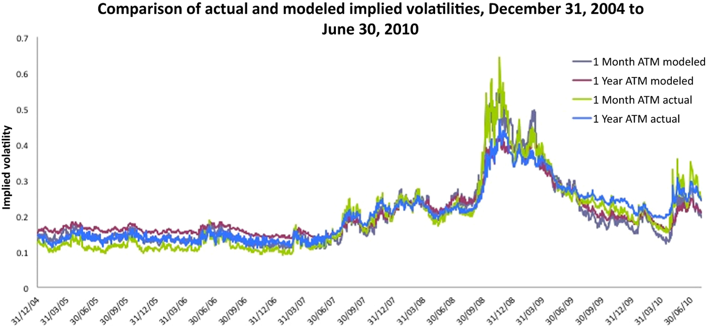
Based on this series, a vector autoregression (VAR) model is estimated to predict implied volatility using historical S&P 500 data, realized volatility, and past implied volatility surface. Figure 1 shows a comparison between actual implied volatilities and implied volatilities derived from the model between December 31, 2004 and June 30, 2010. The model estimates are quite close to the volatilities implied by the market during this period. The model also appropriately captures the spikes in implied volatility levels during the financial crisis in the late 2008.
(colour online) Actual and model predicted implied volatilities. Note: The above figure compares the actual and modeled implied volatilities between December 31, 2004 and June 30, 2010. ATM stands for ‘at the money’.

From this model, we derive implied volatility estimates for the entire historical sample period. For each put option, the implied volatility surface data are interpolated to arrive at the implied volatility corresponding to its strike and maturity. These are then used as inputs to Black–Scholes option pricing model, along with spot values of S&P 500 and risk-free rates, to determine market prices of options on a daily basis from January 31, 1928.
4 Results
4.1 Constant salary growth rate assumption
We simulate the portfolio values under three strategies – unhedged, passively hedged, actively hedged – for hypothetical DC plan participants who are 20 years away from retirement at the beginning of the simulation. Within our sample period, there are 63 such 20-year horizons. These are representative of 63 different DC plan cohort experiences. The first of these cohorts retire in January 1948, which is 20 years away from January 1928, the beginning of our sample period. The last cohort retires in January 2010, the end of our sample period.
We make some assumptions about the participant profile that are held constant for every simulation. The initial value of the portfolio at the beginning of the 20-year horizon is taken as $100,000. The investor's salary income at that point is $60,000 and it is assumed to grow at a fixed rate of 4% per annum till retirement. Regular contributions are made to the retirement account at the rate of 4.5% per annum.
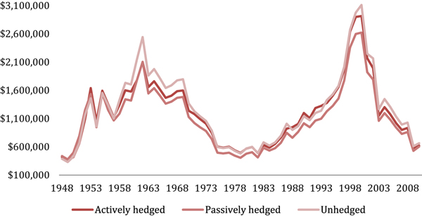
Figure 2 depicts the terminal accumulations over time for DC plan participants who invested in unhedged and hedged (active and passive) portfolios. It is apparent that some of the earlier simulations, which terminate in the late 1940s, represent the experience of the worst-performing investor cohorts in this historical sample period. It does not come as a surprise considering these earlier cohorts confront the full brunt of the Great Depression in the late 1920s and early 1930s. As we move right toward the simulated cohorts retiring in the 1950s, the accumulations progressively improve. A few of these cohorts narrowly escape some of the worst years in the stock market history. While cohorts in the 1960s retire with healthy accumulations, their counterparts between the mid-1970s and mid-1980s face bleak retirement prospects with generally very poor investment outcomes. Again, this is the result of the latter group encountering some of the worst years in stock market, mainly in the 1970s. Thereafter, the cohorts achieve progressively better accumulations reaching a zenith during the turn of the century. The equity market has been so generous to some of these cohorts that their accumulations are many times more than that of the retiring cohorts of the late 1940s.
(colour online) Distribution of simulated retirement wealth between 1948 and 2010. Note: The above figure compares the terminal wealth outcomes of the unhedged and hedged portfolios for different retirement cohorts over the sample period (1948–2010).

In terms of relative outcomes between different cohorts, the overall accumulation profiles of the hedged portfolios are similar to the unhedged portfolio. However, differences are noticeable when comparing contemporaneous simulations for the three strategies. For example, with the hedged strategies, the simulations representing retiring cohorts of the late 1940s still fare the worst. However, the accumulations of these cohorts, while very poor, are still higher than those of the corresponding cohorts under the unhedged strategy. Expectedly, the peaks of the distributions of the hedged strategies are also lower than those of the unhedged strategy.
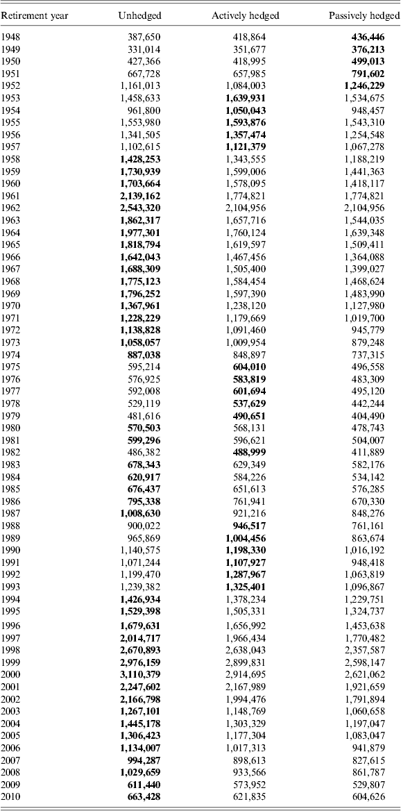
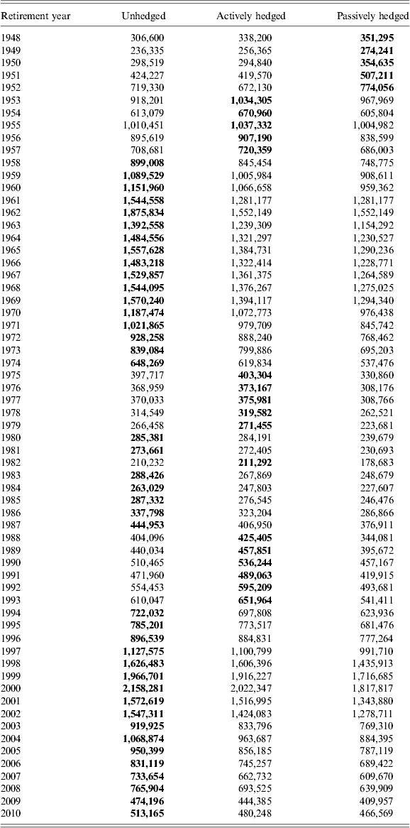
Table 1 shows terminal wealth outcomes under the different strategies (unhedged, actively hedged and passively hedged) for all the 63 simulated horizons. For every retirement year, the highest accumulation among the three strategies is shown in bold. There is a wide range of wealth outcomes between the retirement cohorts. For example, the lowest wealth outcome for the unhedged equities strategy is $331,000 recorded for the cohort retiring in 1949. The same strategy results in almost ten times this wealth for the cohort retiring in 2000, just prior to the tech meltdown.
Terminal wealth of retirement cohorts with constant salary growth

Notes: This table reports the terminal wealth (in dollars) of an unhedged, actively hedged and passively hedged portfolios for different 20-year horizons ending in the month of January of the retirement year indicated in the first column. For every retirement year, the highest accumulation among the three strategies is shown in bold. All simulations are conducted using historical return time-series under the assumption of an initial portfolio of $100,000, salary of $60,000 that grows at a constant rate of 4% per year. The contribution rate is taken as 4.5% of the salary every year.
The wealth outcomes of all strategies are highly correlated with performance of equities during the 20-year horizon i.e., when equity markets do well, accumulation for all the strategies are higher. The correlation coefficients between the terminal wealth outcomes of unhedged equities with those for the passively hedged and actively hedged strategies are nearly 0.99.
In terms of terminal wealth, the unhedged strategy comes ahead of both the active and passive hedging strategies in 41 out of the 63 simulations. The average wealth outcome for the unhedged strategy is 1.27 million dollars. This is almost $168,000 higher than that of the passively hedged strategy. In contrast, the average wealth outcome of the unhedged strategy is higher than that of an actively hedged strategy by a little less than $61,000. The actively hedged strategy resulted in higher wealth on 17 occasions relative to both the unhedged and passively hedged strategies whereas the passively hedged strategy resulted in the higher wealth than the other strategies on five occasions only.
The above simulation results make it clear that historically tail hedging would have proved to be a drag on returns for most DC plan participants. Between the two forms of hedging, the wealth outcomes for an investor who hedged actively would have been higher than one who relied on passive hedging on all but a few occasions. The average wealth difference between the former and the latter exceeds $107,000. This is consistent with the argument made in Bhansali and Davis (Reference Bhansali and Davis2010) that the cost of tail hedging is reduced by actively monetizing the tail hedges when implied volatility rises significantly. When there is a considerable rise in volatility in the short term (lasting few weeks or months) pushing option prices over a pre-set threshold, the active hedging strategy is opportunistic in profiting by selling options acquired cheaply during relatively calm periods. The passive hedging strategy, on the other hand, overlooks this opportunity and is likely to expire worthless on most occasions as markets return to normalcy following short-term turbulence. In such cases, the returns are higher, on average, by pursuing an active rather than a passive approach to hedging.
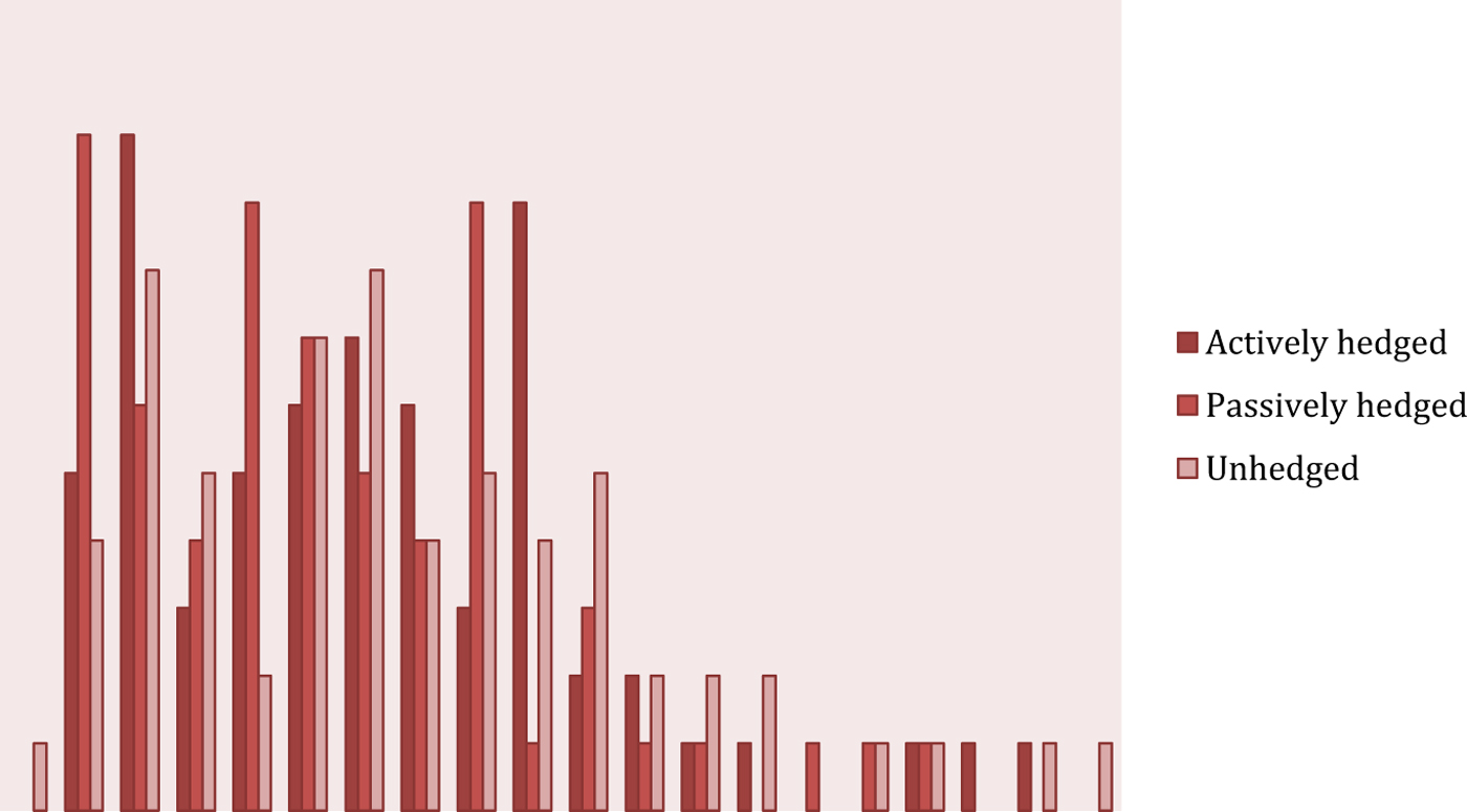
Figure 3 presents the histogram of retirement wealth distribution for all the three strategies. The wealth distribution is wider for the unhedged portfolio compared to the hedged portfolios. It is clear that hedging adds value by truncating the extreme left tail of the distribution but at the cost of giving up the upside in the right tail. It is also evident that active hedging sacrifices far less of the upside of wealth distribution compared to passive hedging whilst not creating any obvious disadvantage on the downside. However, it has to be borne in mind that passive hedging does dominate the other two strategies on a small number of occasions, specifically for the cohorts retiring between 1948 and 1952. Hence its benefits in certain states of the world cannot be ruled out. We discuss this issue in detail in Section 5.2.
(colour online) Retirement wealth distribution of hedged and unhedged portfolios. Note: The above figure shows the terminal wealth distribution of the unhedged and hedged portfolios for different retirement cohorts.

4.2 Variable salary growth rate assumption
In the previous section, we have assumed a constant initial portfolio value, starting salary and salary growth rate for every cohort in our simulations. Now we repeat the simulations for the unhedged and hedged strategies assuming that salary growth for the different cohorts track the observed rate of inflation every year during the sample period. We start with a base salary of $6,000 and initial portfolio of $10,000 in 1928 for our first cohort. These estimates are adjusted with the rate of inflation every year to compute the initial endowment and salary for the subsequent cohorts. For ease of comparison between the retiree cohorts, we report in Table 2 the terminal wealth of different strategies in terms of 2010 dollars.
Terminal wealth of retirement cohorts with variable salary growth

Notes: This table reports the simulated terminal wealth in 2010 dollars of unhedged, actively hedged and passively hedged portfolios for different 20-year horizons ending in the month of January of the retirement year indicated in the first column. All simulations are conducted with historical return time-series under the assumption of an initial portfolio of $100,000, salary of $60,000 that grows every year at a rate tracking the observed rate of inflation in that year. The contribution rate is taken as 4.5% of the salary every year.
While the wealth estimates of the strategies in Table 2 are different from Table 1 (approximately 33% lower average), the relative performance of the unhedged and hedged strategies remains exactly the same. The passive hedging strategy does best for five cohorts (1948–52) while the active hedging strategy results in highest wealth for 17 cohorts (1953–57, 1975–79, 1982, 1988–93). The unhedged strategy dominates the hedged strategies for the remaining 41 cohorts.
5 Further analysis and discussion
5.1 Hedging for worst-case scenarios
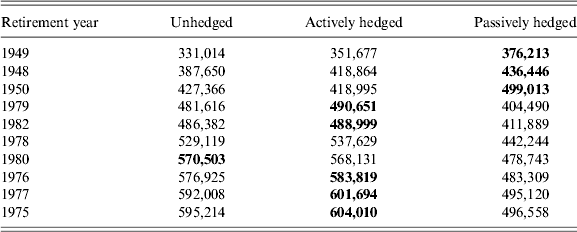
Like all insurance buyers, DC plan participants who consider buying a tail hedge would be more concerned about the performance of hedging strategies in worst-case scenarios than their average performance over all possible scenarios. To analyze this aspect, we look into the performance of the different strategies for the worst-performing cohorts in terms of unhedged equity market returns over 20-year horizons. We pick the ten worst performers among the 63 historical simulations, which are provided in Table 3. For each retirement year, the highest accumulation among the three strategies is shown in bold.
Terminal wealth of ten worst-performing retirement cohorts

Notes: This table presents the ten lowest estimates terminal wealth (in dollars) of unhedged, actively hedged and passively hedged portfolios for cohorts retiring between 1948 and 2010. All simulations are conducted with historical return time-series under the assumption of an initial portfolio of $100,000, salary of $60,000 that grows at a constant rate of 4% per year. The contribution rate is taken as 4.5% of the salary every year.
The average wealth outcomes for the ten worst simulations are less than $423,000, about one-third of the average wealth outcome for all simulations. These represent the retiring cohorts of 1948–50, 1975–80 and 1982. Simulations for cohorts retiring between 1948 and 1950 do capture the massive erosion in market valuation of stocks during the Great Depression commencing with the Wall Street Crash of 1929. However, most of the simulations immediately following this period (i.e., for cohorts retiring in 1951 and thereafter) do quite well in terms of accumulation. These 20-year horizons miss the Wall Street Crash, at least partially, and also benefit more from rising stock market levels in the 1950s. The severe stock market downturn commencing from 1973 and extending to the rest of the decade marked by stagflation also has adverse impact on accumulations for most retiring cohorts during that period.
Interestingly, the simulation results indicate that the cohort retiring in 2009, who encounters the Global Financial Crisis (GFC) and the resulting crash in equity prices, is not among the ten worst-performing cohorts.Footnote 8 It does not come entirely as a surprise given that the final accumulation is a result of performance over 20 years and not just short periods of large gains and losses. Therefore, although the workers retiring in 2009 witness the sharpest fall in equity markets since the Great Depression immediately prior to retirement, they are still much better off compared to the workers retiring in the late 1940s and slightly better off than those retiring in the late 1970s. Similarly, the cohorts of 1973 and 1974 retire with healthy accumulations although there is significant erosion in wealth in the final years before retirement.
How do the hedged strategies perform in the above worst-performing scenarios? On nine of the ten occasions, at least one of the hedged strategies (active or passive) generates higher end wealth than the unhedged strategy. The passively hedged strategy does better than the unhedged strategy for three retirement cohorts: 1948, 1949 and 1950. On two of these occasions, the actively hedged strategy also outperforms the unhedged strategy. However, for another six simulations (1975–79, 1982) where the actively hedged strategy betters the unhedged strategy, the passively hedged strategy falls well short of both.
5.2 Favorable scenarios for tail risk hedging
It is important to explain why the passively hedged strategy dominated the other strategies for the cohorts retiring between 1948 and 1952. By our construction of 20-year horizons, the investment for these cohorts commenced between 1928 and 1930, and encountered heavy losses during the Wall Street crash. This was no ordinary downturn. This was the only instance in history when the US stock market produced negative returns for four successive years (1929–32). The yearly fall in stock market levels between 1929 and 1931 became progressively larger. While the markets somewhat recovered after this string of large losses, there were further large losses down the line, notably during the great crash of 1937. Therefore, it is unsurprising that hedging would prove highly beneficial for the cohorts who experienced all or most of such bad events.
The passive hedging strategy does better than the active strategies for the above simulations because the latter's monetization principle results in selling the hedge too early when the market collapsed (and volatility increased) without anticipating the bigger collapses further down the line. The passive hedging, on the other hand, realize much larger gains by holding the options till maturity. The wealth gains achieved by the passive hedging strategy relative to the unhedged equity strategy for the cohorts retiring between 1948 and 1952 range from 8% to 19%. In comparison, wealth gains achieved by active hedging during the same period only range from 1.5% to 8%.
Next we turn to the simulations where only the actively hedged strategy dominates the unhedged strategy. This is observed between 1975 and 1979 but the wealth gains of the former over latter in every case are less than a paltry 2%. However, during the 1988–1993 periods, the actively hedged strategy produces 3.4% to 7% higher wealth relative to the unhedged strategy. The differences between the wealth gains from active hedging during 1975–79 and 1988–93 are not quite explained by the number of extreme volatility events encountered during the respective 20-year horizons. The cohorts retiring during the mid- to late-1970s encounter more such events leading to monetization of the tail hedge in 1961, 1969 and 1974. In contrast, four of the six retiring cohorts between 1988 and 1993 have tail hedges monetized only on two occasions: 1974 and 1987.
Yet the benefits of active hedging are more pronounced between 1988 and 1993 because of the rapidity with which the extreme events unfold during this period. The market crash (and the jump in implied volatility) on October 19, 1987 is so sharp that the monetization of the hedge occurs at a multiple of 11 i.e., the option pays off 11 times its purchase price within months of its purchase. Had the market decline (and the increase in implied volatility) occurred gradually over a longer period, the monetization of the tail hedge would have been triggered by its market price exceeding our pre-set threshold (five times its purchase price) in a more benign fashion and resulted in less than half the actual pay-off.
The above results shed light on the circumstances under which the hedging strategies add value. Active tail hedging clearly performs well when more extreme volatility events are experienced within one's investment horizon resulting in greater number of pay-offs through monetization. However, its success critically hinges on the rapidity of the fall in equity markets. A quick plunge in the market generally causes panic among investors. As a consequence, implied volatility is pushed up to extremely high levels enabling the strategy to derive a bigger pay-off through monetization. Once monetization occurs, the active hedger hopes the market to quickly stabilize in order to buy a tail hedge at a relatively cheaper price to remain well positioned to benefit from the next extreme event.
Deep and continuous decline in the equity markets, on the other hand, creates problems for active monetization. The experience of cohorts during the Great Depression, when there was a series of extremely large losses, show that active hedging may not offer the best protection in these circumstances. During this type of catastrophic event, when equity markets suffer deep successive losses for several periods, investors are better served by passive hedging strategy, which do not prematurely sell the tail hedges but hold on to them till expiry. However, DC plan participants need to be mindful that this type of events is extremely rare. Therefore, holding a passively hedged position can be expected to act as massive drag on portfolio returns in most situations as our results indicate. It is evident when one considers that even the large losses suffered by equities between 2000 and 2003 does not result in the passively hedged strategies doing better than the unhedged (or the actively hedged) strategy for any other retirement cohorts experiencing those bad events. These losses are nowhere as large as those experienced during the Great Depression and therefore not ‘catastrophic’ enough to benefit from a passively hedged position.
The hedged strategies generally do well compared to unhedged strategy during the periods when markets experience tail events but lag behind during normal periods. Therefore, whether hedging would add value by generating higher wealth at retirement would not only be governed by the occurrence of extreme events but also by the behavior of equity markets throughout the investment life. The experience of the retirement cohort of 2009 in our simulation illustrates this point. This cohort of investors encounters a ferocious tail event in 2008 immediately prior to their retirement. Expectedly, both active and passive hedging produce higher returns than the unhedged strategy during this crisis event. However, the investors with unhedged strategy still end with a higher wealth than those adhering to hedged strategies. It shows that the pay-offs from hedging during the crisis in 2008 (and earlier crash between 2000 and 2002) would not have been large enough to recover the cost of hedging over 20 years between 1989 and 2009.
It is also important to note that the selection of our sample period perhaps underestimate the benefits of hedging, particularly of the passive variety, in a scenario like the Great Depression. The worst-performing cohorts in our simulations i.e., those retiring between 1948 and 1950, were exposed to the biggest stock market collapse in history (1929–37) in the first half of their 20-year horizon. In fact, the first few years (1929–31) of their horizon count among the worst years witnessed in the US stock market. We can only conjecture what might have happened if a collapse of this magnitude occurred in the final years before retirement instead. Given the portfolio value in the years close to retirement is far larger than what it is in the early years, the wealth loss in dollar terms would have been potentially much higher had such a situation been confronted by a few cohorts in our sample. In such a situation, the hedging strategies, especially passive ones, would have outperformed the unhedged strategies by a much larger margin than they have done in some of our simulations.
5.3 Tail risk hedging versus diversification
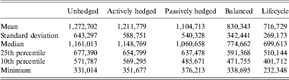
One alternative for investors in hedging portfolio risk is to simply follow a diversified investment strategy. Fixed income securities such as bonds and bills are commonly held by long horizon investors to provide diversification benefits during equity market downturns. To examine how tail risk hedging strategies compare with a simple diversification strategy, we conduct the historical simulations detailed in the previous section with a balanced fund that invests in an annually rebalanced 60:40 portfolio of equities and fixed income. We also repeat the simulations with a lifecycle fund that initially invests in a 100% equities portfolio but linearly switches to a 100% fixed income portfolio over the 20-year horizon. The gradual switching from equities to fixed income assets by lifecycle funds aims to reduce portfolio risk as the investors approach retirement (Viceira, Reference Viceira and Lusardi2008). For both balanced and lifecycle funds in our simulations, the fixed income portion of the portfolio is always equally apportioned between bonds and bills. We use an updated version of the US bonds and bill returns originally compiled by Dimson et al. (Reference Dimson, Marsh and Staunton2002). The key statistics for the terminal wealth distributions of the different strategies are reported in Table 4.
Terminal wealth distribution of different investment strategies

Notes: This table reports the key parameters of the distribution of terminal wealth (in dollars) of different investment strategies. The unhedged, actively hedged and passively hedged portfolios invest in equities only. The balanced portfolio invests in equities and fixed income in a constant 60:40 proportion. The lifecycle portfolio linearly switches from a 100% equities portfolio to a 100% fixed income portfolio over 20 years. The fixed income portion of balanced and lifecycle portfolios are equally apportioned between bonds and bills.
The balanced and lifecycle funds result in far less favorable wealth outcomes for the DC plan investor. Comparing the wealth distributions, the unhedged equity portfolio proves superior to the balanced portfolio at all points except the minimum (worst) outcome, where the latter results in slightly higher terminal wealth. However, both the active and passive hedging strategies always result in higher wealth estimates than those for the balanced fund. The lifecycle fund fares even worse with the mean, median, 25th percentile, 10th percentile, and minimum wealth outcomes significantly lower than the corresponding estimates of the unhedged and hedged strategies.
However, a comparison between the average or corresponding percentiles of the wealth distribution does not rule out that the balanced or the lifecycle portfolios resulting in superior wealth outcome compared to the unhedged or hedged equity positions for certain cohorts. We examine this issue by comparing the final wealth outcomes under the different strategies cohort by cohort between 1948 and 2010 although we do not present the detailed results here.Footnote 9 Out of the 63 simulated cohort outcomes, the balanced and the lifecycle fund result in a higher wealth outcome compared to the unhedged equity strategy on only one and four occasion(s), respectively. When we compare the wealth outcomes with those of the hedged strategies, the balanced fund is ahead of the passive and active hedging strategies on 16 and 2 occasions, respectively. The corresponding estimates for the lifecycle fund are 13 and 3, respectively.
We pay particular attention to the ten worst-performing cohorts with lowest accumulations for the unhedged strategy as shown in Table 2. For these cohorts, the balanced and the lifecycle fund improve the wealth outcomes on only one and two occasions, respectively. This is a disappointing result given these funds are often perceived to provide cushion against poor equity market performance. Among the hedging alternatives, the active hedging strategy outperforms the balanced fund outcomes for all ten cohorts and the lifecycle fund outcomes for nine cohorts. The passive hedging strategy does not enjoy such dominance as it results in lower wealth outcomes for five and seven cohorts compared to the balanced and the lifecycle funds, respectively. However, for cohorts retiring between 1948 and 1950 who experienced the deepest declines in the equity market during the Great Depression, the passively hedged portfolio outperforms the balanced and lifecycle portfolios by a large margin. In terms of the average terminal wealth for the ten worst-performing cohorts, the balanced and lifecycle funds do worse compared to the unhedged as well as both the hedged strategies. Based on this evidence, one can conclude that diversification strategies appear to be inferior to hedging strategies in guarding against poor outcomes in the equity market.
5.4 Volatility and drawdown estimates
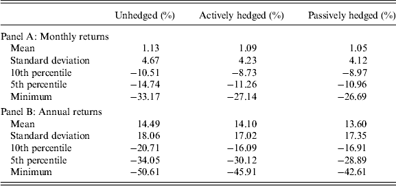
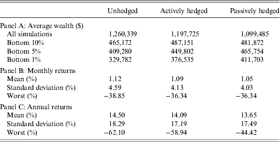
So far, we have focused on the risk of encountering extreme market events and consequently retiring with less wealth. But risk is often equated with short term uncertainty and volatility in portfolio returns. Therefore, it is appropriate to measure return volatility over time as well as large declines between two consecutive periods (drawdowns). From this viewpoint, a strategy would be considered riskier if the investor experience higher return volatility over their investment horizon or large negative returns over a month or year. For each simulation, we compute the mean and standard deviation of both monthly and annual returns. The average estimates for 63 simulations are provided in Table 5. Additionally, we show the 10th percentile, 5th percentile and the worst returns for these historical simulations.
Return, volatility and drawdown estimates of historical simulations for all retirement cohorts

Note: The mean return and standard deviation in panels (A) and (B) are computed for each simulation and then averaged for all 63 simulations.
As expected, the unhedged strategy has a higher mean return and standard deviation than both the hedged strategies. The poorest monthly and annual returns, as apparent from the 5th, 10th, and the minimum outcomes, are also higher on average for the unhedged strategy. When comparing the hedged strategies, active hedging produces higher mean return on average than passive hedging. It is expected given the generally higher outcomes of active hedging observed in our previous results for retirement wealth.
The volatility comparisons of the two hedging strategies, however, are striking. The results indicate that although active hedging would have resulted in slightly higher standard deviation of monthly returns, yet in terms of annual returns, the standard deviation would have been lower than passive hedging. This is possibly explained by the mean reversion in volatility i.e., a jump in volatility during crisis events subsequently drops as panic among investors subsides. Compared to passive hedging, the monthly variation in returns for active hedging strategy is more affected by the short term rise in volatility during crisis periods as it liquidates the tail hedge. However, over the long term, as volatility reverts, active hedging returns become more stable.
Turning to the poorest returns, passive hedging does better than the active strategy in terms of the minimum and 5th percentile monthly and annual returns but not in terms of 10th percentile returns. It is consistent with our earlier results which show that in all but the poorest of equity market conditions, active hedging yields superior results compared to the passive hedging strategy.
5.5 Sensitivity to calendar effect
One issue that deserves closer attention is the starting (and ending) point of each 20-year period. The results of individual simulations could be sensitive to the selection of the start date, particularly if a tail event is positioned very close in the time series to the start or end date of the 20-year period. For example, if a major market crash occurs immediately before the start date (or immediately after the end date) of a simulation, the wealth outcome would be more favorable to the unhedged strategy because the simulation period would miss that bad event because of our choice of start date. On the other hand, if such extreme events coincide with the start and end dates of our simulations, the hedging strategies would appear better than they would have otherwise. All our rolling historical simulations for retirement cohorts start and end in January. To test whether our inference on overall effectiveness of different strategies is robust to any kind of calendar effect, we conduct further simulations by randomizing the start date i.e., each simulation randomly selects the start date of the 20-year block from the historical time series between 1928 and 2010. The process is repeated 1,000 times and the simulation results are summarized in Table 6.
Wealth, return and volatility estimates of simulations with randomized starting dates

Note: The mean return and standard deviation in panels (B) and (C) are computed for each simulation and then averaged for all 63 simulations.
The results of the randomized simulations do not change our previous inferences about the different strategies using fixed start dates. In terms of average wealth outcome for all simulations, the unhedged strategy dominates the hedged strategies, with active hedging doing better than passive hedging. When equity returns are very poor, the benefit of hedging becomes apparent. For the lowest 10% equity market outcomes, both active and passive hedging results in higher terminal wealth than the unhedged strategy, with the latter producing greater relative benefits as we move to the poorest (worst 5% or below) outcomes. Similar to the historical simulations with fixed start dates, the maximum portfolio loss over a single year is lowest for the passive hedging strategy. Also, like our results in Table 5, the passive and active hedging strategy has the lowest standard deviation of monthly and annual returns respectively.
5.6 Sensitivity to monetization threshold
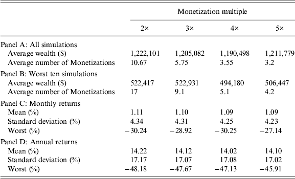
We also examine the sensitivity of active hedging outcomes to the monetization threshold by repeating the historical simulations for active hedging strategy using monetization thresholds of 2, 3 and 4 i.e., the option is monetized whenever its value reaches two, three and four times of its respective purchase price. The results are reported below in Table 7. For comparison, we also include the active hedging results using our original monetization multiple of 5. The estimates provided are the averages for the number of the simulations conducted under each multiple.
Active hedging strategy outcomes for different monetization multiples

Note: The mean return and standard deviation in panels (C) and (D) are computed for each simulation and then averaged for all 63 simulations.
The results show that active hedging with lower monetization thresholds generally result in higher average wealth outcomes. (The exception is 4× threshold which has lower average final wealth than 5× threshold.) The average final wealth of the retiring worker, however, is not overly sensitive to the choice of the monetization multiple, the difference between the highest (2× threshold) and the lowest (4× threshold) outcomes being less than 3%. All four strategies record higher average wealth outcomes compared to passive hedging but fall short of the unhedged strategy. However, when we examine the worst ten simulation periods, the active hedging strategies become dominant. For each of these simulations, the unhedged strategy is outperformed by at least two active hedging strategies in terms of final wealth outcomes. The passive strategy is outperformed in nine out of ten occasions, in many cases by all the active hedging strategies. Between the active strategies, the 2× and 3× monetization thresholds produce higher average wealth for the worst simulation periods than those with higher thresholds.
The number of monetization events is far higher for 2× and 3× thresholds compared to 4x or 5x thresholds. This result is as per expectation as lower monetization thresholds make the active hedging strategies more opportunistic in cashing in on smaller jumps in implied volatility. The hedging strategies with higher thresholds, on the other hand, have to wait for a substantial rise in implied volatility to derive any pay-off from monetization.Footnote 10 Over a long investment horizon, a strategy with a lower threshold would potentially have a large number of small pay-offs relative to a strategy with higher threshold, which would have a small number of large pay-offs. The dominance of one over the other for a specific investment period, therefore, would depend on both the frequency and severity of the tail events within that period. For example, if equity returns are generally poor over a period without being extremely volatile, a lower monetization rule would perform better as it would be able to capitalize on smaller rises in implied volatility. Actively hedged strategies with higher thresholds have to wait for a bigger jump in implied volatility to monetize and such events are relatively infrequent. This phenomenon is apparent in the results for the worst ten simulations for unhedged equities, many of which are characterized by gradual stock market declines over long periods (i.e., during the 1970s) rather than sharp market crashes associated with big jumps in implied volatility. As a consequence, we find actively hedged strategies with lower monetization thresholds faring better in these situations.
Whilst in terms of average returns, our historical sample period appears to be more favorable towards hedging strategies with lower monetization thresholds, the trade-off comes in the form of higher volatility of returns for these strategies both on monthly and annual basis (as shown in panels (C) and (D)) compared to active strategies with higher threshold as well as passive strategies. Also, the worst monthly and annual portfolio losses generally get higher as the monetization threshold is lowered. However, the volatility reduction benefits are apparent even for strategies with very low thresholds. For example, the actively hedged portfolio with 2× monetization threshold has a slightly lower standard deviation of returns (but also marginally lower average returns) compared to the unhedged portfolio. In terms of the worst monthly and annual returns, the 2× strategy easily outperforms the unhedged counterpart.
6 Conclusions
Tail Hedging has been getting increased attention from practitioners to shield portfolios against extreme events in the market. However, there is skepticism about the benefits of these hedges for long horizon investors. We have presented evidence based on long-term historical pay offs from tail risk hedging strategies to shed light on this debate. We show that whilst buying tail hedges would have proved beneficial in some cases, the misgivings about these strategies among long horizon investors are not unfounded. Extreme or tail risk events, by very definition, are events with low probability of occurrence. Most retirement cohorts in our simulations do not experience more than two or three such events over a 20-year period. But since the timing of these events is unpredictable, the portfolios are required to remain hedged all the time. It entails a significant cost which in many cases, even when extreme events are encountered, outweighs the benefits resulting in lower wealth in retirement.
About the superiority of active tail hedging over its passive counterpart, we find that the former would have outperformed the latter for all except a few retirement cohorts in the past. On an average, active hedging would have resulted in higher wealth for equity investors compared to passive hedging. Yet this evidence in itself is insufficient to adjudge it as superior form of protection against tail events for two reasons. First, the cohorts in our sample that experienced the worst equity market conditions in history (the Great Depression) and retired with lowest wealth levels would have been better off by adopting the passive hedging strategy. In contrast, the 20-year periods when active hedging outperforms the unhedged strategy, the overall performance of the equity market is far from catastrophic. Second, although relative to passive hedging, active hedging outperforms the unhedged equity strategy on many more occasions, it does so by a much smaller margin. This suggests that whilst active hedging would have enabled the employees to retire with higher wealth on certain occasions, it may not have made a huge difference to their financial situation. In contrast, passive hedging would have made a more significant difference to the retirement wealth cohorts for whom it worked best i.e., those retiring between 1948 and 1950. Moreover, one can argue that the benefit of passive (and too some extent, active) hedging has been underestimated in our results since none of the cohorts in our historical sample encountered an event as severe as the Great Depression in the final few years before retirement when the portfolio size is significantly larger.
Importantly, we identify the circumstances in which one strategy would be more successful relative to others. As with all insurance purchases, buying tail hedges does not pay off in the absence of extreme events i.e., when markets are calm over long periods. In these situations, both active and passive hedging yield the same results as options expire worthless. Hedging may also drag returns significantly if extreme events are few and far apart. Active hedging yields greatest benefits when the market crashes happen in short, sharp spells. The temporary rise in risk perception drives up implied volatilities and allows for profitable monetization. Irrational panic selling in fearful markets is almost always accompanied by significant rise in implied volatility levels in the short term and therefore, creates the best pay-offs for active hedging. In our sample, the 1987 crash when equities fell by 23% on a single day (Black Monday) was the single-most profitable event for active hedging.
Since passive hedging does not involve selling the hedge when they rise in value, short term turbulence in the market does not benefit the strategy. Instead this type of hedging works best when the market suffers a series of losses over a relatively longer time period. Such events are more likely to be driven by deep economic recessions rather than investors reacting in panic to one-off disaster events. The results of our historical simulations suggest that for passive hedging to outperform an unhedged strategy over long horizons, bear markets encountered in the course of business cycles are not sufficient. In our sample, the only retirement cohorts who would have found passive hedging to be the most beneficial of all strategies were the ones who experienced the extraordinary market decline during the Great Depression when equity values continued to fall over several years.
We also find that the outcome of active hedging is dependent on the selection of monetization threshold. Lowering the threshold pushes the return and volatility of the actively hedged strategy towards those of an unhedged equity portfolio. One may argue that setting the monetization threshold too low is not designed to protect against tail events marked by extreme volatility but to cash on during periods of relatively minor spikes in volatility. Interestingly, in our simulations, lower monetization thresholds not only resulted in higher average wealth but also fared better during the worst 20-year periods of equity returns in our historical sample. It highlights the fact that historically the greatest danger to the long horizon investors’ wealth accumulation has not been posed by rare and catastrophic market crashes like the Black Monday (when higher monetization rules derive maximum benefits due to severe rise in volatility) but by long periods of depressed equity markets as experienced during the 1970s. However, if investors hold the view that extreme events like the Black Monday may occur more frequently in the future than in the past, they would be more inclined to hedge actively using a higher monetization threshold. Also, since lower thresholds enforce a larger number of monetization events (i.e., more selling and buying of options) over the investment life, higher transaction costs can act as a deterrent.
Overall, our findings indicate that historically holding hedged positions would have proved costly for most DC plan participants. For two out of every three cohorts in our sample period, hedging would have resulted in reduced wealth in retirement. One important consideration is the fact that investment horizons for the plan participants get progressively shorter with approaching retirement. If purchasing tail hedge is considered to be more effective over short horizons than over long horizons, then it would imply that employees should buy more tail hedge when they are nearing retirement and less when they are farther away from it. This leads to an investment principle where they hold unhedged positions when young but allocate more funds towards tail hedging as they get older. Such a strategy would lessen the impact of market shocks close to retirement and may potentially generate some additional returns through active hedging if extreme volatility events unfold precisely during that period.
A limitation of our study is that we do not consider the variation in plan contributions due to employment breaks. Impact on accumulations may vary as a result of timing and frequency of unemployment spells experienced by different cohorts. The relationship between the timing of shocks in the equity market and the labor market, as posited by studies like Seligman and Wenger (Reference Seligman and Wenger2006), can alter the risk-return tradeoff of tail hedging. Also, there are other strategies available to DC plan participants like varying contributions following tail events or even deferring the timing of their retirement. Future research should look into the relative costs and benefits of tail risk hedging vis-à-vis such actions by participants.