







1. Introduction
A yield stress fluid (YSF) keeps its shape like a solid until a sufficiently large stress ( $>\sigma _{Y}$) initiates a liquid-like flow (Coussot et al. Reference Coussot, Nguyen, Huynh and Bonn2002; Bonn et al. Reference Bonn, Denn, Berthier, Divoux and Manneville2017). Such YSFs are widely found in biofluids (cell medium and mucus) (Hu et al. Reference Hu, Bian, Grotberg, Filoche, White, Takayama and Grotberg2015), as well as in various industries, such as paintings, cosmetics and foods. For YSFs, the solid-to-liquid change is the key flow behaviour commonly denoted as yielding (Møller, Fall & Bonn Reference Møller, Fall and Bonn2009; Balmforth, Frigaard & Ovarlez Reference Balmforth, Frigaard and Ovarlez2014; Malkin, Kulichikhin & Ilyin Reference Malkin, Kulichikhin and Ilyin2017; Coussot Reference Coussot2018; McConnell et al. Reference McConnell, Ortiz, Sutherland, Newell, Grillet, McMaster, Bhakta and Rao2022; Dey et al. Reference Dey, Ortiz, Cleaves, McMaster, McConnell, Tjiptowidjojo, Grillet, Secor, Newell and Rao2023) or fluidization (Bocquet, Colin & Ajdari Reference Bocquet, Colin and Ajdari2009; Benzi et al. Reference Benzi, Divoux, Barentin, Manneville, Sbragaglia and Toschi2019, Reference Benzi, Divoux, Barentin, Manneville, Sbragaglia and Toschi2021; Garg et al. Reference Garg, Bergemann, Smith, Heil and Juel2021; Jadhav, Rossi & Karimfazli Reference Jadhav, Rossi and Karimfazli2021). The yielding depends on the strain rate and stress, and shows a gradual transition rather than a sudden event (Oldroyd Reference Oldroyd1947; Bonn & Denn Reference Bonn and Denn2009; Coussot & Rogers Reference Coussot and Rogers2021). Since plastic deformation takes place after elastic response, stress overshoot appears as a consequence of microstructural rearrangement, and transient/permanent shear banding follows due to its inhomogeneity (Benzi et al. Reference Benzi, Divoux, Barentin, Manneville, Sbragaglia and Toschi2021).
Contrary to yielding, which is a transition from solid to liquid under stress exceeding  $\sigma _{Y}$, solidification in YSFs represents a liquid-to-solid transition as stress decreases below
 $\sigma _{Y}$. The disparity between dynamic and static yield stresses suggests that the solidification process differs fundamentally, requiring a distinct analytical approach (Divoux, Barentin & Manneville Reference Divoux, Barentin and Manneville2011; Chaudhuri, Berthier & Bocquet Reference Chaudhuri, Berthier and Bocquet2012; Balmforth et al. Reference Balmforth, Frigaard and Ovarlez2014). Solidification processes have been studied across diverse contexts, ranging from time-dependent simple shear scenarios to the cessation of motion in particles, bubbles, and droplets (Huilgol, Mena & Piau Reference Huilgol, Mena and Piau2002; Matson & Hogg Reference Matson and Hogg2007; Tokpavi, Magnin & Jay Reference Tokpavi, Magnin and Jay2008; Tsamopoulos et al. Reference Tsamopoulos, Dimakopoulos, Chatzidai, Karapetsas and Pavlidis2008; Sikorski, Tabuteau & de Bruyn Reference Sikorski, Tabuteau and de Bruyn2009; Dimakopoulos, Pavlidis & Tsamopoulos Reference Dimakopoulos, Pavlidis and Tsamopoulos2013; Damianou et al. Reference Damianou, Philippou, Kaoullas and Georgiou2014; Jalaal et al. Reference Jalaal, Seyfert, Stoeber and Balmforth2018; Huilgol, Alexandrou & Georgiou Reference Huilgol, Alexandrou and Georgiou2019). It has been shown that the criteria for cessation are influenced by factors including yield stress, stress during solidification, surface tension, and relaxation time. Given its prevalence in capillarity-driven flows like wetting, coating, spreading and wicking (Huilgol & Kefayati Reference Huilgol and Kefayati2018), solidification warrants specific attention within the scope of capillary imbibition. While a few models address the flow dynamics of YSFs during solidification (Bertola Reference Bertola2009; Géraud et al. Reference Géraud, Jørgensen, Petit, Delanoë-Ayari, Jop and Barentin2014; Huilgol & Kefayati Reference Huilgol and Kefayati2018; Balmforth Reference Balmforth, Ovarlez and Hormozi2019) and compare them with experimental results (Balmforth, Ghadge & Myers Reference Balmforth, Ghadge and Myers2007; Jalaal, Stoeber & Balmforth Reference Jalaal, Stoeber and Balmforth2021; van der Kolk, Tieman & Jalaal Reference van der Kolk, Tieman and Jalaal2023), mostly they focus on the asymptotic solution for the final state (
 $t \rightarrow \infty$). Notably, none has been compared directly with the experimental dynamics throughout the entire wetting process.
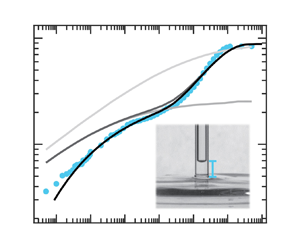
In this work, our primary focus is the solidification of YSFs in capillary rise (figure 1a). From the conservation of momentums acting on the liquid (density  $\rho$), the wall shear stress on a capillary inner surface with a sufficiently narrow radius
 $R$ is a function of rise height (
 $h(t)$) as expressed by
 \begin{equation} \sigma_{w}(t)=\frac{{\varGamma}\cos \theta_{E}}{h(t)}-\frac{\rho gR}{2}, \end{equation}
with the constitutive equation for Newtonian and shear thinning fluids,
 \begin{equation} \dot{h}(t)=\frac{R}{s+2}\left(\frac{\sigma_{w}(t)}{K}\right)^{s-1}, \end{equation}
where  ${\varGamma }$ is the surface tension of the liquid–air interface,
 $\theta _{E}$ is the equilibrium contact angle between the liquid and the capillary,
 $g$ is the gravitational constant,
 $K$ is the consistency parameter,
 $n$ is the thinning power, and
 $s=1/n+1$ (Lucas Reference Lucas1918; Washburn Reference Washburn1921; Rideal Reference Rideal1922). Equation (1.2) can be generalized for the Newtonian fluid by putting
 $n=1$ and
 $K$ as the viscosity. Because
 $h(t)$ increases in time,
 $\sigma _{w}(t)$ finally converges to zero for typical constitutive equations (Newtonian or shear thinning fluid). This corresponds to a monotonic rise curve of aqueous glycerol in figure 1(b). The YSFs, however, undergo solidification at
 $h_{p}={\varGamma }\cos \theta _{E}/(\sigma _{Y}+\rho gR/2)$, the height where
 $\sigma _{w}=\sigma _{Y}$ (Balmforth Reference Balmforth2022). We found that the solidification slows down YSFs at
 $h_{p}$, but is followed by another onset of capillary rise, as in figure 1(c). This contradicts a previous study that says a YSF stops at
 $h_p$ (Géraud et al. Reference Géraud, Jørgensen, Petit, Delanoë-Ayari, Jop and Barentin2014). Instead, slip attributes the flow after the solidification. Our proposed model predicts the complete capillary rise of YSFs quite accurately, and explains what determines the flow dynamics after solidification based on the relevant length and time scales.
(a) Schematic for the capillary rise experiment. Capillary rise  $h(t)$ of (b) 85
 $\%$ glycerol (Newtonian fluid,
 $\sigma _{Y}=0$) and (c) 0.12 wt.
 $\%$ Carbopol (YSF,
 $\sigma _{Y}=10$ Pa). Dashed lines in (b,c) are (1.1) combined with (1.2) for Newtonian and simple power law fluids (
 $\sigma _{Y}=0$), respectively. The solid line is (1.1) with (2.1). The shading is an error bar. Experimental parameters follow table 1.

2. Results and discussion
Figure 1(b) shows that Newtonian fluids show a monotonic increase until reaching equilibrium height ( $h_{E}=2{\varGamma } \cos \theta _{E}/\rho gR$), where Laplace pressure is balanced by gravity (see Appendix A for experimental details). The model curve aligns with Newtonian fluid data when Hagen–Poiseuille flow is assumed. However, in figure 1(c), the model fails to match for YSFs with a simple power-law fluid, possibly due to the presence of yield stress and inability to account for yielding or solidification impacts.
Accordingly, a well-known Herschel–Bulkley (HB) model is implemented to replace (1.2). For  $\sigma >\sigma _{Y}, \sigma =\sigma _{Y}+K\dot {\gamma }^{n}$, where
 $\dot {\gamma }$ is the shear rate. When
 $\sigma \le \sigma _{Y}$,
 $\dot {\gamma }=0$. The apparent rise velocity
 $\dot {h}(t)$ is obtained by averaging the shear rate in radial direction:
 $\dot {h}(t)=\int _{0}^{R}2{\rm \pi} r\,\dot {\gamma }(r,t)\,{\rm d} r$ (Sochi & Blunt Reference Sochi and Blunt2008; Pérez-González et al. Reference Pérez-González, López-Durán, Marín-Santibáñez and Rodríguez-González2012). By replacing the shear rate with the HB model, it rearranges and explicitly links
 $\dot {h}(t)$ to the wall shear stress (
 $\sigma _{w}(t)$) as
 \begin{equation} \dot{h}_{HB}(t)=R\left(\frac{\sigma_{w}(t)}{K} \right)^{s-1}f(\epsilon(t),s), \end{equation}
where
 \begin{equation} f=(1-\epsilon(t))^s\left\{\frac{(1-\epsilon(t))^2}{s+2} +\frac{2\epsilon(t)\,(1-\epsilon(t))}{s+1}+\frac{\epsilon(t)^2}{s}\right\}, \quad \epsilon(t)=\frac{\sigma_{Y}}{\sigma_{w} (t)}<1. \end{equation}
For regime  $\epsilon (t)\ge 1$,
 $\dot {h}=0$. Upon applying
 $\epsilon =0$, (2.1) reduces to (1.2), where
 $f$ becomes
 ${1}/({2+s})$.
With the implementation of (2.1), the numerical solution with measured  $\sigma _{Y}$ is shown as a solid line in figure 1(c) (see Appendix B for the rheology measurement result). The plateau height, denoted as
 $h_{p}$, was determined precisely by the model. This indicates that the plateau is a result of the solidification process of the YSF. For all the theoretical curves, dynamic contact angle (DCA) theory is employed to account for the wetting friction of the meniscus (Kim et al. Reference Kim, Lim, Lee and Choi2020). The DCA description and its fitting are available in Appendix C and figures 5(a,b) below. The YSF surface tension is estimated from the Laplace pressure at
 $h_{E} = h(t\rightarrow \infty )$ due to the lack of reproducibility of the previously proposed method, which heavily relies on the selection of geometry (Jørgensen et al. Reference Jørgensen, Le Merrer, Delanoë-Ayari and Barentin2015; Jalaal et al. Reference Jalaal, Stoeber and Balmforth2021). The measured surface tension is given in table 1, where its value varies by polymer concentration. These values can be considered as apparent surface tensions acting on a capillary imbibition system, since the value can be hindered dynamically by the yield stress (Martouzet et al. Reference Martouzet, Jørgensen, Pelet, Biance and Barentin2021).
Rheological properties and slip layer thicknesses:  $\sigma _{HB}$ is fitted from a rheology measure, while
 $\sigma _{Y}$ is fitted from capillary rise
 $h(t)$. Theoretical prediction follows
 $\sigma _{Y}$.

Interestingly, stress overshoot has negligible impact on the macroscale dynamics of capillary rise. Recent experimental and theoretical studies have demonstrated that the transition from solid to liquid is accompanied by a stress overshoot, as evidence of plastic deformation of YSF (Donley et al. Reference Donley, Singh, Shetty and Rogers2020; Kamani, Donley & Rogers Reference Kamani, Donley and Rogers2021). In a case of the capillary rise, the good fit of (2.1) to the initial rising speed indicates that stress overshoot has little effect on the macroscale flow dynamics; with a sufficiently large Laplace stress ( $\sigma \sim 100$ Pa) at the beginning, the characteristic time scale for yielding rate (
 ${\sim }10^{-2}$ s) is an order of magnitude faster than the time scale of our measurements (
 ${\ge }10^{-1}$ s) (Benzi et al. Reference Benzi, Divoux, Barentin, Manneville, Sbragaglia and Toschi2021).
As shown in figure 1(c), the experimental curve of YSFs shows a significant deviation from the saturation predicted by (2.1) (solid line) and continues to rise until  $h_{E}$. Derived from (1.1), which is relevant to all instances of capillary rise irrespective of the fluid's rheological characteristics, it is observed that the wall shear stress diminishes with an increase in penetration length. Hence the rise beyond
 $h_{p}$ is indicative of a decline in wall shear stress. Ultimately, this anomalous flow behaviour is associated with the culmination of the liquid-to-solid transition, during which shear stress continues to decrease even after surpassing
 $\sigma _{Y}$. This makes solidification distinct from the re-entrance effect under long-term creep tests (Landrum, Russel & Zia Reference Landrum, Russel and Zia2016) and thixotropic aging (Choi, Armstrong & Rogers Reference Choi, Armstrong and Rogers2021). One possibility is that YSFs may not undergo complete solidification, as seen in the analogy of delayed yielding (Landrum et al. Reference Landrum, Russel and Zia2016). This approach emphasizes the rheological inhomogeneity of YSF and incorporates local mobility as a function of shear stress and shear rate (Benzi et al. Reference Benzi, Divoux, Barentin, Manneville, Sbragaglia and Toschi2021). Another possibility is that a YSF flows after
 $h_{P}$ as a ‘gliding solid block’. The experiments can be explained by the presence of a shallow lubrication layer near the wall, where high shear stress is concentrated. The slip of YSFs is common, regardless of their yielding mechanism, chemical composition, geometry or wall surface roughness (Piau Reference Piau2007; Damianou et al. Reference Damianou, Philippou, Kaoullas and Georgiou2014; Zhang et al. Reference Zhang, Lorenceau, Basset, Bourouina, Rouyer, Goyon and Coussot2017; Jalaal et al. Reference Jalaal, Seyfert, Stoeber and Balmforth2018).
In order to verify the aforementioned hypotheses, the flow velocity is visualized with the particle image velocimetry (PIV) method. We expect a plug flow in the case of an entire solid, otherwise a curved velocity profile for a mixed solid–fluid state. An example optical image is shown in figure 2(a). Experimental details for PIV measurement are given in Appendix D. The velocity profile was analysed during horizontal imbibition due to its convenience of imaging. This method remains valid as a YSF solidifies even in the absence of gravity, and the penetration curve exhibits a plateau similar to that of the vertical rise (figure 2b). The velocity profile depicted in figure 2(c) is indeed a plug, suggesting that the fluid undergoes complete solidification instead of existing in a state of mixture between solid and liquid.
(a–c) Slip demonstration of horizontal imbibition using 0.12 wt.  $\%$ Carbopol. (a) Microscope image of 0.12 wt.
 $\%$ Carbopol inside a glass capillary. The solution is seeded with 10
 $\mathrm {\mu }$m hollow glass spheres. The scale bar is 100
 $\mathrm {\mu }$m. The scheme on the right describes the depletion layer at the YSF–glass interface. (b) Horizontal capillary imbibition curve. (c) The PIV analysis result. The solid line is the plug flow velocity profile from the bulk imbibition speed. (d,e) Stress-velocity plots during the vertical capillary imbibition for (d) 0.12 wt.
 $\%$ and (e) various YSFs. The solid line is the Newtonian slip model (2.4). The shading in (d) shows the error bar. Insets in (c,d) show the vertical capillary rise curve
 $h(t)$, and coloured markers denote corresponding regimes. Velocity in (e) is normalized with
 $\mu$ and
 $l_{s}$. The concentrations in the legend in (e) are given in wt.
 $\%$.

To confirm the slip effect, the wall shear stresses are examined from all the points after the plateau. Because the wall shear stress can be computed simply by the rise ( $h$) using (1.1), it is independent of the constitutive relationship to the fluid viscosity. In figure 2(d), when the height of the vertical capillary rise is converted into the wall shear stress, it shows the wall shear stress increases linearly with the rise velocity. Even if the experimental stress at the regime with high velocity shows a higher value than the theoretical prediction, it lies in the theoretical model when the lower bound of the error bar is accounted for. Moreover, the same relation has been found even more clearly in other vertical capillary rises of xanthan solutions (grey markers in figure 2e), as well as other YSFs shown in Zhang et al. (Reference Zhang, Lorenceau, Basset, Bourouina, Rouyer, Goyon and Coussot2017). In other words, even if the apparent viscosity changes, YSFs share similar slip behaviour at boundaries.
To implement slip, a Newtonian slip model (Zhang et al. Reference Zhang, Lorenceau, Basset, Bourouina, Rouyer, Goyon and Coussot2017) is added to (2.1). The slip layer has thickness  $l_{s}$, in which polymers are depleted. When its viscosity is assumed as the solvent viscosity (
 $\mu$), the slip velocity can be written with wall shear stress proportionally as
 \begin{equation} \dot{h}_{slip}(t)=\frac{l_{s}\sigma_{Y}}{\mu\,\epsilon(t)}, \end{equation}
which is added to  $\dot {h}_{HB}(t)$ as
 \begin{equation} \dot{h}(t)=\dot{h}_{slip}(t)+\dot{h}_{HB}(t). \end{equation}
Even though other slip models have been suggested in Damianou et al. (Reference Damianou, Philippou, Kaoullas and Georgiou2014), it has been demonstrated that these various models converge to a linear model when the edge evaporation effect is removed (Zhang et al. Reference Zhang, Lorenceau, Basset, Bourouina, Rouyer, Goyon and Coussot2017). Therefore, in our evaporation-controlled study, we consider the linear model, which still shows great accordance with experimental data within the error range.
Equation (2.4) is connected with (1.1), and the value of  $l_{s}$ is determined by fitting the slope in the stress–velocity plot, the linear plot of figure 2(d). The slip gradually develops even before solidification when
 $h< h_{p}$, but the slip's effect on the rising speed is negligible as
 $\sigma _{Y} \ll \sigma _{w} (t)$. After the solidification, the slip itself takes on the role of the apparent speed as the YSF is not flowing, considering that the contribution from (2.1) is zero with
 $\sigma _{w} (t)<\sigma _{Y}$. Due to the discontinuity of (2.1) between regimes before and after
 $h_{p}$, the numerical calculation explicitly connects the two regimes. The final solution of the early regime, which includes
 $h$,
 $\dot {h}$ and
 $\sigma _{w}$, serves as the initial condition after
 $h_{p}$.
In figures 3(a,b), the solid lines represent the capillary rise prediction of (1.1) and (2.4) for different YSFs. The experimental data are plotted using colour markers to indicate the yield stress. The rheological properties, surface tension and  $l_{s}$ are given in tables 1 and 2. Surprisingly, model curves are capable of effectively capturing the diverse dynamics of capillary rise. The transition from solidification to gliding flow is accurately described smoothly, as supported by experimental results.
(a,b) Proposed model prediction (solid lines) against experiments. From top to bottom, concentrations are 0.08 and 0.12 wt.  $\%$ in (a), and 0.3, 0.7, 1.0 and 1.3 wt.
 $\%$ in (b). Marker colours match the colour map for
 $\sigma _{Y}$. (c,d) Normalized numerical solutions of (1.1) and (2.4) varying yield stress and slip conditions. From the bottom, (c)
 $\sigma _{Y} = 40$, 10 and 2 Pa, while (d)
 $(l_{s},\phi ) = (0.01\ {\rm nm},0.006)$, (0.2 nm, 0.1) and (16 nm, 9) nm. Dashed lines in (c,d) are shear thinning curves without slip. (e) Contour plot of
 $\varDelta$. The solid line shows
 $l_{s} = 10$ nm, and the dashed line is
 $l_{s}=0.1$ nm. The lower inset is the graphical definition of
 $\varDelta$, while the upper inset shows the same contour over
 $l_{s}$ versus
 $\sigma _{Y}$. For (c–e), rheological properties other than
 $\sigma _{Y}$, surface tension and DCA parameters follow the Carbopol 0.12 wt.
 $\%$ values shown in table 1 and table 2.

To better reflect the initial trajectory of 1.3 and 1.0 wt.  $\%$ xanthan solutions, the yield stress was fitted empirically from the rise curve. This is due to the ambiguity in the yield stress determination for xanthan (Barnes & Walters Reference Barnes and Walters1985; Tang et al. Reference Tang, Kochetkova, Kriegs, Dhont and Lettinga2018). The residual discrepancy can be explained with shear banding, as shown in Appendix E. By reducing the shear banding effect with salt (Tang et al. Reference Tang, Kochetkova, Kriegs, Dhont and Lettinga2018), experimental data follow the proposed model very well. To be within the scope of this work, accurate prediction of shear banding (de Souza Mendes Reference de Souza Mendes2011) is not included here. Although the Carbopol 0.08 wt.
 $\%$ sample's yield stress is also fitted, a plateau curve appears and could be interpreted with our proposed model, when the surface is altered into a less slippery condition through surface silanization (see Appendix E and figure 6b). The lowest concentration for which Carbopol maintains yield stress characteristics is 0.08 wt.
 $\%$, as highlighted by Jaworski et al. (Reference Jaworski, Spychaj, Story and Story2022), suggesting potential shear thinning behaviour under rapid flow conditions. Under conditions of a slippery surface, initial penetration speed is notably quicker compared to scenarios involving a silanized surface, where the pace significantly diminishes. The yield stress values
 $\sigma _{Y}$, deduced from the
 $h(t)$ profiles, are used for the theoretical prediction in figures 3(a) and 3(b), with values listed in table 1. Concurrently, the table also presents
 $\sigma _{HB}$ values, derived from rheological analyses detailed in Appendix B.
The plateau shows diverse intensities and shapes in both our experiments and the theoretical model. It can be expected that a larger yield stress results in a stronger plateau. In figure 3(b), the plateau at 1.3 wt.  $\%$ xanthan solution in the darkest colour marker, however, is less pronounced and nearly unnoticeable as compared to the lower concentrations. It can be inferred that the strength of a plateau might be determined not solely by the yield stress, but also by other variables such as slip and consistency parameter (
 $K$).
Based on the proposed model, the various intensities and shapes of the plateau are studied theoretically. Capillary rise curves were obtained in figures 3(c) and 3(d) by changing only the rheology or slip, respectively, in order to distinguish the effects from each factor. All axes are normalized, where  $\hat {h}$ is the rise height divided by the final height (
 $h_{E}$), and
 $\hat {t}$ is the time divided by the characteristic time scale of capillary rise (
 $t_{v}$, which is defined without yield stress and given in table 2) (Kim et al. Reference Kim, Lim, Lee and Choi2020).
DCA model parameters, slip dominance and plateau intensity.

In figure 3(c), an increase in the yield stress slows down the rise speed, and the plateau appears earlier. Figure 3(d) depicts the variation of slip strength while assuming a constant yield stress. In order to assess the contribution of slip at the plateau, the velocity ratio ( $\phi$) is obtained by dividing the slip contribution (
 $\dot {h}_{slip}$) by the non-slip contribution (
 $\dot {h}_{HB}=\dot {h}-\dot {h}_{slip}$). At the point where the slip and non-slip velocities experience the same stress around the plateau, (
 $\sigma _{w}=2\sigma _{Y}$), we have
 \begin{equation} \phi={\frac{\dot{h}_{{slip},\epsilon=0.5}}{\dot{h}_{{HB},\epsilon=0.5}}}= \frac{8\,g(n)\,l_{s}}{R\mu } {\left(\frac{K}{{\sigma_{Y}}^{1-n}} \right)}^{1/n}, \end{equation}
where  $g(n)={(n+1)(2n+1)(3n+1)}/{n(7n^2+8n+2)}$. The two graphs (figures 3c,d) are completely different, suggesting that each has a unique impact on the capillary rise dynamics. The position of the plateau and the transitional rate of rise are determined mainly by the yield stress, whereas the persistence of solidification and the rate of later rise are affected by slip.
The time scale for the duration of the plateau ( $t_{p}$) is derived via dividing plateau height by slip velocity, as
 \begin{equation} t_{p}=\frac{h_{p}}{\dot{h}_{{slip},\epsilon=1}} =\frac{h_{E} \mu}{l_{s}\sigma_{Y}\left(1+\dfrac{2\sigma_{Y}}{\rho gR}\right)}. \end{equation}
We define  $\hat {t}_{p}$ as
 $t_{p}$ divided by
 $t_{v}$, shown by dots on the solid lines in figures 3(c) and 3(d). Solidification finishes faster for higher yield stress and more slippery cases. It is interesting to note that when
 $l_{s}$ is reduced below a single atomic size,
 $t_{p}$ extends beyond
 $10^3$ s. According to Zhang et al. (Reference Zhang, Lorenceau, Basset, Bourouina, Rouyer, Goyon and Coussot2017), this duration is sufficient for the evaporation-induced residual stress to build up at the edge. The evaporation at the edge slows down the capillary imbibition speed because it affects primarily the wetting friction of the meniscus (Zhao et al. Reference Zhao2019). In Young's spreading of YSFs on rough surfaces, a similar cessation occurs when the plateau phase persists long enough for the meniscus edge to fully dry out (Géraud et al. Reference Géraud, Jørgensen, Petit, Delanoë-Ayari, Jop and Barentin2014). Our observation of additional flow and its interpretation by incorporating the slip model distinguish our findings from the previous models and experiments (Balmforth Reference Balmforth2022), where lubrication theory is applied identically in Hele-Shaw cell geometry. On the other hand, the previous no-slip asymptotic rise curve can be derived from the present model by assuming an extremely short
 $l_{s}$ and minimizing the DCA effect.
For a general understanding of the plateau intensity, we evaluated the flexion of plateau ( $\varDelta$) as
 \begin{equation} \varDelta = \int_{0}^{\infty}({\tilde{h}_0(\tilde{t})- \tilde{h}(\tilde{t})})\,{\rm d} \tilde{t}, \end{equation}
where  $\tilde {t}$ and
 $\tilde {h}$ are logarithmic
 $\hat {t}$ and
 $\hat {h}$, and
 $\tilde {h}_0$ is the normalized logarithmic rise height with
 $\sigma _{Y}=0$. As shown in the bottom inset
 $h(t)$ curve of figure 3(e),
 $\varDelta$ is the integration of the difference in height between curves
 $\tilde {h}_0$ and
 $\tilde {h}$. The intensity is calculated by varying
 $\sigma _{Y}$ and
 $l_{s}$ as shown on the plane of the normalized plateau time and height. According to the presented phase diagram, it can be observed that the plateau strength is positively correlated with the magnitude of the yield stress, while exhibiting an inverse relationship with the degree of slip. Even if the solidification occurs early (low
 $\hat {h}_{p}$), the flow can closely resemble the dynamics of shear thinning fluids when they experience a large slip effect (low
 $\hat {t}_{p}$), as well as in high
 $\hat {h}_{p}$ cases. The enhancement of slip can be obtained in cases of the increasing thickness of the slip layer (e.g. the enhancing repulsive forces between the YSF element and the smooth wall).
3. Conclusions
This study revisits the capillary imbibition problem in yield stress fluids (YSFs), demonstrating that YSFs inevitably solidify during wetting or spreading flows as the velocity gradually diminishes. The liquid–solid transition appears as a plateau at the rise curve, at a glance, but its re-rise occurs by a slip between the YSF and the inner wall surface. By assuming a depleted slip layer, the entire capillary rise curve could be predicted with a simple rheology model. The MATLAB code utilized for numerical calculations is readily accessible. Even if our demonstration is performed under ideal conditions without evaporation, the suggested model including DCA theory can provide crucial information about how YSFs flow inside channels at lower stresses, which is difficult to measure accurately, typically requiring a complicated force sensor or a micro-PIV device (Graziano et al. Reference Graziano, Preziosi, Uva, Tomaiuolo, Mohebbi, Claussen and Guido2021). Our capillary imbibition model with experiments can be helpful to obtain parameters such as surface tension, slip length and dynamic wetting coefficients, required for wetting, spreading, simple pipe flow and any other slippery flow. Since predicting penetration rate and fluid uptake in porous media shares the same phenomena with capillary rise, our system can also provide clues for modelling YSF flow in porous media.
Acknowledgements
We are grateful to S. Han and the Korea Institute of Geoscience and Mineral Resources (KIGAM) for helpful discussions, and K.H. Kim and K. Lee for their comments on the manuscript.
Funding
This research was supported by the Basic Science Research Program through the National Research Foundation of Korea (NRF) (NRF-2021R1A6A3A13046176, NRF-2021R1A2C2009859, RS-2023-00276535) and the Korea Evaluation Institute of Industrial Technology (20014762).
Declaration of interests
The authors report no conflict of interest.
Code availability statement
The code proposed in this study is openly available in github at https://github.com/hanull15/capillary_ysf.
Appendix A. Experimental capillary rise measurement
Capillary rise experiments are performed using a glass capillary;  $h(t)$ and
 $\theta (t)$ measurements and glass preparation follow our previous work, Kim et al. (Reference Kim, Lim, Lee and Choi2020). A borosilicate glass capillary was purchased from World Precision Ins. (Sarasota, FL). The aq. glycerol data shown in figure 1(b) are from a capillary with radius 0.42 mm. Other capillary radius conditions are given in table 1. The glass capillary was properly cleaned with a 1 M sodium hydroxylate (NaOH) solution at 75
 $^\circ$C, and rinsed with deionized water. Wet capillaries are dried in a vacuum oven for more than 1 hour. A CCD camera (EO-0413M 1/3
 $"$ CMOS monochrome USB camera, 59-363 Edmund Optics) is used to record capillary rise video at a rate of 20 frames per second. Evaporation is prevented by enclosing the experimental set-up within an acrylic box equipped with a humidifier. During the capillary rise experiment, the YSF in the reservoir was not subjected to any additional shearing actions, like stirring or vortexing.
Purchased from Lubrizol and Sigma, respectively, Carbopol 940 NF polymer and xanthan are dissolved in water at concentrations between 0.08 wt.  $\%$ and 1.3 wt.
 $\%$. Polymeric solutions were mixed with a magnetic stirring bar under moderate rpm below 300 to prevent the scission of polymer strain, which is well known as critical for hindering viscoplastic properties (Dinkgreve et al. Reference Dinkgreve, Fazilati, Denn and Bonn2018). To fully hydrate the polymers, mixing is continued for more than 24 hours. Afterwards, the Carbopol solution pH is matched to 7 by adding 1 M NaOH drops to make the polymer strain swollen and have yield stress.
Appendix B. Rheology measurement
In figures 4(a–c), the stress–strain rate ( $\sigma \unicode{x2013}\dot {\gamma }$) flow curve of the YSFs was measured using an MCR302 (Anton Paar Ltd) with a sandblasted PP25 plate. Before each test, all YSFs were pre-sheared with a stirring bar and rested for more than 1 hour to minimize the effect of shear history and obtain reproducibility. Shear stress is measured by controlling the shear rate, with the time interval between rates determined by reaching a steady state where stress stabilizes within a tolerance
 ${\le }1\ {\rm nN} \ {\rm m}$, typically averaging approximately 5 seconds. The initial deviation seen in ramp-up curves from the HB model corresponds to the elastic response phase. As figure 4(a) demonstrates, the minimal discrepancy between up-ramp and down-ramp above yield stress suggests that all samples behave as simple YSFs devoid of thixotropic properties. The minor fluctuation in xanthan solution shear rates ranging from 0.1 to 1 s
 $^{-1}$ is likely due to local plastic deformations or multiple stress overshoots, reflecting the inherent microstructural inhomogeneity of the xanthan solution, even after adequate mixing. These fluctuations minimally impact capillary rise because the solid-to-liquid plastic deformation primarily occurs rapidly at the initiation of the measurement, and the shear rate diminishes over time, similar to a ramp-down approach. Although ramp-up data are presented to clearly depict the fit with the
 $\sigma _{HB}$ model, the capillary rise process adheres to the HB curve fitted, as illustrated in figure 4(a). Measured parameters are detailed in table 1, and the rheological behaviour of aqueous glycerol is consistent with Kim et al. (Reference Kim, Lim, Lee and Choi2020), with the solvent viscosity set at 1 mPa s.
(a) Ramp-up and ramp-down cycles of shear-rate–stress measurement for Carbopol 0.12 wt.  $\%$. The inset is the corresponding stress–stress curve. Solid lines are for power 1. (b,c) The measured up-ramp cycles of shear rate versus stress flow curves for (b) Carbopol and (c) xanthan solutions. Concentrations in (b,c) are given in wt.
 $\%$.

Appendix C.The DCA models
The DCA models describe the deviation of Laplace pressure from that at equilibrium ( $h=h_{E}$) (Cox Reference Cox1986). Thus the wetting friction is defined for the meniscus as
 \begin{equation} \varTheta(t)=2{\rm \pi} R {\varGamma}(\cos{\theta_{E}}-\cos{\theta(t)}). \end{equation}
In this paper, two different DCA models are combined for YSFs. Before the solidification, wall shear stress is assumed to be significantly larger than yield stress, working as shear thinning fluids:
 \begin{equation} \varTheta_{t}(t)=-\chi_{1}\,\frac{K}{R^{n-1}} \left(\frac{\dot{h}(t)}{\theta(t)}\right)^{n}, \end{equation}
where  $\chi _1$ is a fitting parameter (Kim et al. Reference Kim, Lim, Lee and Choi2020). After
 $h_{p}$, the wetting friction is assumed to be proportional to the slip stress as
 \begin{equation} \varTheta_{s}(t)=-\chi_{2} 2 {\rm \pi}R \, d (t)\, \sigma_s (t) =-\frac{\chi_2 R \mu}{l_s}\,\frac{1-\sin{\theta(t)}}{\cos{\theta(t)}}\,\dot{h}(t), \end{equation}
where parameter  $\chi _2$ is the proportional factor,
 $\sigma _{s}$ is the slip shear stress at the meniscus, and
 $d$ is the meniscus depth. When
 $\chi _1$ and
 $\chi _2$ are fitted from contact angle change (figures 5a,b) against capillary rise velocity, the DCA prediction agrees well with the experimental early rise velocity as shown in figures 3(a,b). Since the shear thinning model does not account for yield stress, the transition from simple shear DCA model to slip DCA model appears as a discontinuity at the solidification (
 $\sigma _{w}=\sigma _{Y}$).
(a,b) The contact angle change during the capillary rise of (a) xanthan and (b) Carbopol. (c1,d1) The raw meniscus images of (b) before and after solidification. (c2,d2) The corresponding contact angle measurement results. The measurement method is validated in Kim et al. (Reference Kim, Lim, Lee and Choi2020).

Appendix D. The PIV measurement
We purchased 0.001 wt.  $\%$ of 10
 $\mathrm {\mu }$m sized hollow glass sphere from Sigma and added to 0.12 % Carbopol. By conducting the same shear-rate–stress measurement given in Appendix B, we checked that the rheological properties of solution is not changed. The focus of image given in figure 2(a) is at the vertical midplane of the horizontal capillary by matching the focus plane to the capillary inner wall accurately. For the supply of fluid at the capillary end, the solution reservoir is placed at the same vertical height with the capillary. A polystyrene petri dish is used, with a hole on the wall to expose the solution's free surface to the capillary inlet.
Appendix E. The effects of shear banding and surface conditions
The deviation of the rise curve between xanthan solutions and our model prediction might be due to the localization of fluidity, commonly known as shear banding. Shear banding appears as bands of different shear rates even if the entire fluid is under the same stress in simple Couette flow. This is known to be attributed to the inhomogeneity in the microstructure pronounced in polymeric gels.
To minimize the shear banding effect on xanthan solutions, the applied shear stress during capillary imbibition was delocalized by the addition of 5 and 10 mM NaCl Tang et al. (Reference Tang, Kochetkova, Kriegs, Dhont and Lettinga2018). As NaCl concentration increases, capillary imbibition aligns with the numerical model (figure 6a). This indicates that the shear banding effect could decelerate the initial stage of the capillary imbibition.
(a) Salt effects on the capillary imbibition of xanthan solutions. (b) Capillary rise on surfaces without (circle) and with (triangle) the APTES modification. The insets in (a,b) are the same curves in linear scale.

Also, we explored the capillary rise behaviour under a surface condition that is well known as no-slip. As emphasized in the main text, slip behaviour is crucial to understand the entire dynamics of capillary imbibition ( $h(t)$). To further support the proposed theoretical model, we prepared silanized glass capillaries by adsorbing (3-Aminopropyl)triethoxysilane (APTES) to the surface of initial silanol. Dried capillaries were soaked in 5 v/v
 $\%$ APTES anhydrous acetone solution (Kiernan Reference Kiernan2015). Because of high reactivity of APTES with water, silanization was conducted in a sealed vial without exposure to ambient humidity. The identical contact angles of the inner capillary surfaces indicated the homogeneity of the axial surface treatments.
A plateau region is observed at the APTES-modified surface as triangle markers in figure 6(b). By changing the surface to be less slippery,  $l_{s}$ decreased from 15 to 1 nm, and the plateau intensity (
 $\varDelta$, see main text for description) increased from 0.4 to 1.3. This shows that the surface well known as no-slip can also be described with extremely small
 $l_{s}$, thus the plateau appears regardless of the surface condition, including slippery and chemically or physically modified surfaces.
Although the previous study (Jalaal, Balmforth & Stoeber Reference Jalaal, Balmforth and Stoeber2015) suggested that silanization could be an effective method to correct slip, it seems to be not valid for the faster flow condition. In order to suppress slip behaviour, the silanized ( $-\mathrm {NH}^{3+}$) surface should strongly attract negatively charged polymers; however, it will fail to create no-slip conditions in fast flows where hydrodynamic stress surpasses microscale electrostatic force. Salt dissolved in solutions could also weaken the electrostatic force. Moreover, slip correction using a rough surface frequently fails at pressure-driven pipe flow (Liu & de Bruyn Reference Liu and de Bruyn2018) and at flow near a falling sphere (Holenberg et al. Reference Holenberg, Lavrenteva, Shavit and Nir2012). This evidence supports that the plateau may appear commonly in capillary imbibition with varying surface charges or roughnesses. Previous experimental studies on surface conditions named with no-slip might be the result of a shallow slip layer (
 $l_{s}$) close to the size of a single solvent molecule (
 $\le$1 nm), following the dashed line in figure 3(c) of the main text.
For the APTES-modified surfaces, adjustments in model parameters were necessary:  ${\varGamma }=35 {\rm mN}\ {\rm m}^{-1}$,
 $\theta _0 =54^{\circ }$ and
 $\chi _1 = 3.5$. The reduction in hydrophilicity decreased Laplace pressure, consequently lowering the final rise height. Differences in surface tension values could be attributed to meniscus evaporation, acting as an additional frictional force (Zhang et al. Reference Zhang, Lorenceau, Basset, Bourouina, Rouyer, Goyon and Coussot2017). The experiment did not use a humidifier for APTES-treated capillaries in order to prevent the formation of condensed water droplets on the glass surface, which would otherwise form an additional meniscus and negate Laplace pressure.


 Open access

