

INTRODUCTION
Temporal frequency distributions, typically created by plotting frequencies of radiocarbon ages over time or through the use of summed calibrated radiocarbon probability distributions, are often used as proxies for prehistoric population density, following from the assumption that there is a linear relationship between population density and the amount of dateable material in the archaeological record. One major complication to this method, however, is the distortive impact of the loss of sedimentary records due to erosion, or what is known as taphonomic bias. Taphonomic effects typically lead to there being higher frequencies of young things and lower frequencies of older things in the geologic and archaeological records. This can skew distributions so that they appear to show a rapid climb in frequencies towards the present, even if there was no true change in abundance through time (Surovell and Brantinhgam, 2007; Surovell et al., Reference Surovell, Finley, Smith, Brantingham and Kelly2009). Without proper correction, such taphonomically distorted curves most likely do not represent true demographic signals.
This paper and prior studies (Surovell and Brantingham, Reference Surovell and Brantingham2007; Surovell et al., Reference Surovell, Finley, Smith, Brantingham and Kelly2009; Williams, Reference Williams2012; Shennan et al., Reference Shennan, Downey, Timpson, Edinborough, Colledge, Kerig, Manning and Thomas2013; Surovell and Pelton, Reference Surovell and Pelton2016) seek to counter this problem by developing models of taphonomic bias that can used to subtract taphonomic effects from temporal frequency distributions and make visible the underlying population signal. The method developed by Surovell et al. (Reference Surovell, Finley, Smith, Brantingham and Kelly2009) is based on the assumption that the best indicator of relative human population density is not the absolute abundance of archaeological materials over time but, instead, the frequency of cultural material relative to the frequency of geologic contexts in which those materials can occur. In other words, if archaeology is common relative to geology for a particular slice of time, then population densities were high. This method can used to reconstructed relative population densities through time.
The Surovell et al. (Reference Surovell, Finley, Smith, Brantingham and Kelly2009) method for taphonomic correction uses a nonlinear function fit to a database of 1849 radiometric dates from volcanic contexts (Bryson et al., Reference Bryson, Bryson and Ruter2006):
 $$n_{t} {\equals}7.726{\times}10^{6} (t{\plus}2176.4)^{{{\minus}1.3925}} $$
where n t is the predicted number of geologic contexts from time t, expressed in yr BP, where the present is defined as AD 1950 in accordance with the radiocarbon convention. To correct for taphonomic bias, relative population density is estimated as the number of archaeological sites that date to a particular time interval, say 4.5 to 4.0 ka, divided by the value of that equation at the midpoint of that time interval. Williams (Reference Williams2012) proposed a slight modification of that equation to account for systematic regression fitting errors in the most recent and oldest time periods.
These results offered a preliminary method for correcting taphonomic bias and revealing clearer demographic signals within temporal frequency distributions and were subsequently applied by a number of researchers (e.g., Munoz et al., Reference Munoz, Gajewski and Peros2010; Peros et al., Reference Peros, Munoz, Gajewski and Viau2010; Gajewski et al., Reference Gajewski, Munoz, Peros, Viau, Morlan and Betts2011; Kelly et al., Reference Kelly, Surovell, Shuman and Smith2013; Williams, Reference Williams2013; Williams et al., Reference Williams, Veth, Steffen, Ulm, Turney, Reeves, Phipps and Smith2015). Given the fact that this function (Eq. 1) was derived from a single database of dates taken from solely volcanic contexts, however, we felt that it would be prudent to develop an independent database of radiocarbon ages from terrestrial geologic contexts as a cross-check on such results. Furthermore, the publication of the IntCal13 radiocarbon calibration curve (Reimer et al., Reference Reimer, Bard, Bayliss, Beck, Blackwell, Bronk Ramsey and Buck2013) offers refinement of the radiocarbon timescale and therefore additional incentive to revisit that work.
This project therefore follows the Surovell et al. (Reference Surovell, Finley, Smith, Brantingham and Kelly2009) and Williams (Reference Williams2012) publications by attempting to independently replicate those models of taphonomic bias. We use identical methods by creating an independent database of 2457 radiometrically dated materials, generating a nonlinear function to characterize it, and then statistically comparing these data to those contained in the Bryson et al. (Reference Bryson, Bryson and Ruter2006) dataset. Independent corroboration of the Surovell et al. (Reference Surovell, Finley, Smith, Brantingham and Kelly2009) and Williams (Reference Williams2012) models of taphonomic bias would instill greater confidence in their usage in the reconstruction of prehistoric demographic trends from temporal frequency distributions.
METHODS
We created a global database of radiocarbon ages (n=2457) by systematically gathering ages from papers published in the journals Quaternary Research (1995–2015) and Quaternary International (1989–2017). We refer to this as the “Quaternary Sample”. These journals were chosen because they provide international coverage spanning the Pleistocene and Holocene. We do not consider our database to be exhaustive but do feel it is a sufficient sample for addressing the question at hand. Because our intent was to create an independent geologic dataset for use in the correction of archaeological frequency distributions, we only included dates from contexts that were non-archaeological and non-volcanic. We also excluded contexts that are largely immune to erosional forces, such as samples from lacustrine, bog, and marine contexts, as well as those from caves and rock-shelters. The majority (54.6%) of ages are from North America (n=1341) and the remainder are distributed across all other continents to the exclusion of Antarctica. The ages are derived from a variety of materials, including soil organic matter and organic sediments (32.9%), plant micro- and macrofossils (25.2%), charcoal (23.5%), bone apatite and collagen (10.1%), carbonates including mollusk shell (4.8%), and other (3.5%).
The other dataset used in this project, the “Volcanic Sample,” is that of Bryson et al. (Reference Bryson, Bryson and Ruter2006). It is a compilation (n=1849) of radiocarbon ages from volcanic contexts and also is global in distribution. These two datasets share a total of five individual ages and are essentially independent.
The raw ages of the Quaternary and Volcanic datasets were calibrated using the IntCal13 calibration curve (Reimer et al., Reference Reimer, Bard, Bayliss, Beck, Blackwell, Bronk Ramsey and Buck2013) in OxCal v. 4.3 (Bronk Ramsey, Reference Bronk Ramsey2009). Median ages were calculated for each age as the midpoint of the 1-sigma calibrated age ranges. Both datasets include ages as young as 49.5 yr BP and as old as >50 ka, but we trimmed them to only include ages between 1 and 40 ka. We removed the ages on the young end because all temporal frequency distributions of radiocarbon ages show a drop in frequencies toward the present in the most recent time intervals, a shift which is almost certainly due to a bias against the submission of near surface radiocarbon samples (Surovell et al., Reference Surovell, Finley, Smith, Brantingham and Kelly2009). We trimmed ages older than 40 ka because small amounts of modern contamination in ancient samples produce ages in the 40 to 50 ka range (Taylor, Reference Taylor1987:116).
To create best-fit taphonomic models, calibrated radiocarbon ages were binned in 250-yr intervals, and following Surovell et al. (Reference Surovell, Finley, Smith, Brantingham and Kelly2009), power functions n t =a (t+b) c were fit to each using the nls function in R v.3.4.2Footnote 1 . As shown in Surovell et al. (Reference Surovell, Finley, Smith, Brantingham and Kelly2009), this function performs better than other models (e.g., exponential, inverse) at explaining the long-term taphonomic trend. Statistical comparisons of datasets were done using chi-squared and Kolmogorov-Smirnov tests.
RESULTS
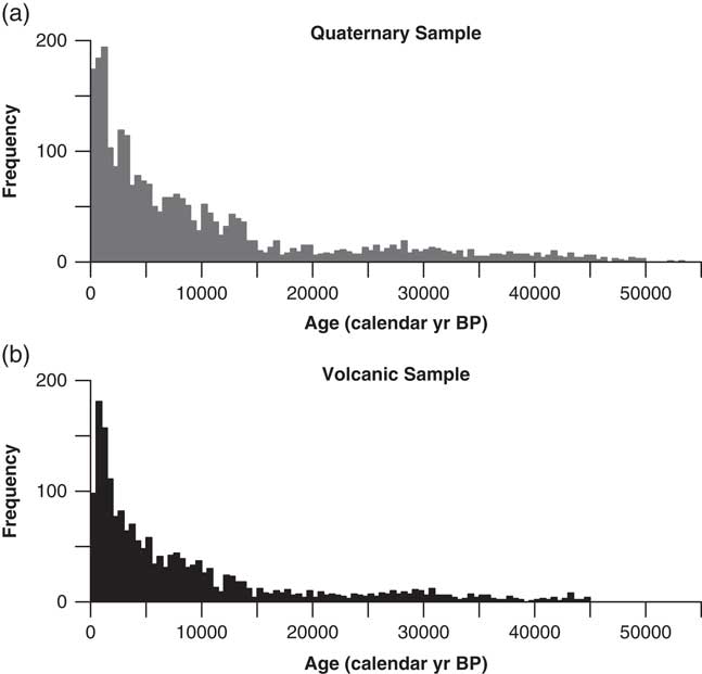
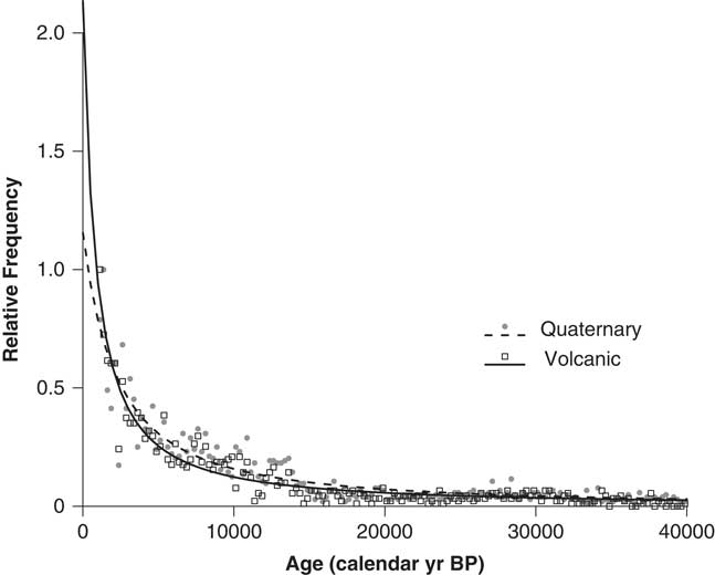
Temporal frequency distributions for both datasets are shown in Figure 1. Both datasets show the expected pattern of nonlinear increase in ages toward the present. Likewise, both datasets show a decline in date frequencies in the most recent time intervals (<1 ka). For each trimmed dataset (1 to 40 ka), we standardized date frequencies to the maximum number of ages occurring within a 250-yr bin. When plotted on the same scale, these curves appear to be virtually identical (Figure 2). Though the datasets appear visually similar, they differ significantly in distribution (two-sample KS test, D=0.0774, P<.001). To determine the time periods where these two datasets diverge, we binned the ages in 1000-yr intervals and performed a chi-square test. This test confirmed that the datasets are statistically different (X2=57.76, df=38, P=.021). We further found that the differences are largely driven by the first (1 to 2 ka) and last (39 ka to 40 ka) time intervals; ages contained within the volcanic dataset are overrepresented on the younger end, while the Quaternary dataset is overrepresented on the older end. These differences are likely driven by variations in dataset construction and research bias, as discussed above.
Frequency distributions of the (a) Quaternary and (b) Volcanic datasets.

Nonlinear regression best fit curves for the Quaternary and Volcanic datasets.

For the time interval from 2 to 39 ka, we obtain mixed results. A chi-squared test shows no significant difference between the two datasets (X2=42.85, df=36, P=.20), whereas a two-sample KS test suggests that they differ (D=.0653, P=.001). Large sample sizes are likely influencing statistical analysis, however results suggest that these distributions are very similar in overall form, while differing slightly in shape. Best fit models for each dataset after standardization to the bin of maximum frequency produce very similar curves (Figure 2). Best fit functions for the Quaternary, Volcanic, and Combined data sets are:
 $${\rm Quaternary}\,\,\colon\,n_{t} {\equals}85502.321\,(t{\plus}3149.004)^{{{\minus}1.392}} $$
 $$\hskip-1.2pt{\rm Quaternary}\,\colon\,n_{t} {\equals}85502.321\,(t{\plus}3149.004)^{{{\minus}1.198}} $$
 $$\hskip-18pt{\rm Combined}\,\,\colon\,n_{t} {\equals}21149.57(t{\plus}1788.03)^{{{\minus}1.26}} $$
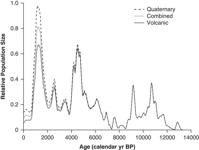
All three curves converge on similar values for ages older than 2 ka, but separate for younger ages. The Volcanic curve has a y-intercept at 2.13, while the Quaternary curve intersects the y-axis at a value of 1.15. The combined curve has an intermediate value (y-intercept=1.69). It should be noted that these intercepts are extrapolated beyond the limits of the datasets that were used to estimate them, and which curve bests describes the reality of the worldwide relative abundance of sediments of different ages over this time period is difficult to know with present information. Divergent results for the last two millennia are expected, depending upon which curve is used. To demonstrate how the use of each curve affects population reconstructions, in Figure 3 we present a reconstruction of relative human population size over the last 13 ka in the Bighorn Basin of Wyoming. Data were taken from Kelly et al. (Reference Kelly, Surovell, Shuman and Smith2013). For ages older than 6 ka, the three population reconstructions are virtually identical. Minor differences are evident from ca. 6 to 2 ka, after which the curves diverge. Although overall population trends remain unchanged, estimated relative population sizes for the Late Prehistoric period (~1500 to 250 yr BP) vary substantially depending upon which curve is used.
Taphonomically corrected summed probability distribution of archaeological radiocarbon dates from the Bighorn Basin, Wyoming using the Quaternary, Volcanic, and Combined models. Data taken from Kelly et al. (Reference Kelly, Surovell, Shuman and Smith2013).

DISCUSSION AND CONCLUSION
Using a large sample of terrestrial geologic radiocarbon ages, we were able to replicate the original taphonomic curve of Surovell et al. (Reference Surovell, Finley, Smith, Brantingham and Kelly2009), although minor differences in the shapes of the distributions may be present. These curves diverge in the last few thousand years, with the largest differences occurring the last millennium. Because two independently compiled samples of radiocarbon ages produce essentially the same curves with only minor variations, it gives us confidence that these curves are at least representative of the distribution of Quaternary studies over time.
Temporal frequency distributions of radiocarbon ages are a product of both the natural distribution of sediments globally and how they are sampled. Whether the sum product of scientists working in the Quaternary is a random or representative sample of sedimentary contexts occurring naturally is unknown, although we feel strongly that there is research bias present against the sampling and dating of recent sediments. There may also be bias causing the overrepresentation of certain time periods that garner a lot of academic attention, like the Younger Dryas. To know whether these distributions mimic the natural age distribution of sediments on the planet would require a true random sampling regime (i.e., randomly sampling and dating sedimentary contexts globally). In the absence of such information, we recommend continuing the use of these curves for taphonomic correction. This suggestion comes with the caveats that, of course, it will remain difficult to apply these methods to recent periods and there are likely other factors like research bias affecting archaeological temporal frequency distributions (Ballenger and Mabry, Reference Ballenger and Mabry2011), the extent to which frequencies of radiocarbon dates relate linearly to human population size (Freeman et al., Reference Freeman, Byers, Robinson and Kelly2017), and regional variation in taphonomic processes.
Our recommendation is that if researchers continue to use these methods in archaeological demographic reconstruction, they use the Combined Model presented in this paper because it is based on the largest sample of ages (n=4306). We also recommend the exploration of regional variation in taphonomic processes and the creation of regionally specific curves for more precise taphonomic correction.
ACKNOWLEDGMENTS
We thank Tim Jull and one anonymous reviewer for their helpful comments.
SUPPLEMENTARY MATERIAL
To view supplementary material for this article, please visit https://doi.org/10.1017/qua.2018.78