1. Introduction
Thermal convection is a pervasive phenomenon found in a wide variety of natural and engineering processes (Lappa Reference Lappa2009). Examples include motion of the Earth’s molten core, atmospheric and oceanic dynamics and solar phenomena. A common approximation in fundamental studies of convection is that all fluid parameters are constant except for the fluid density in the buoyancy force (Drazin & Reid Reference Drazin and Reid2004; Lappa Reference Lappa2009; Chandrasekhar Reference Chandrasekhar2013). This is the Oberbeck–Boussinesq approximation, valid in many physical situations, which allows systems to be described by the incompressible Navier–Stokes equations subject to a buoyancy force and an advection–diffusion equation for the temperature field. The canonical problem is Rayleigh–Bénard convection, which focuses on flow fields driven by buoyancy and confined between two infinite horizontal plates. Rayleigh–Bénard convection was an early study of hydrodynamic instability in which a given flow configuration is unstable at certain wavenumbers as a control parameter is varied. In this case, the control parameter is the Rayleigh number
 $\mathit{Ra}$
characterizing the relative strength of buoyancy-driven inertial forces to viscous forces. In atmospheric and solar environments, estimates of
 $\mathit{Ra}$
are typically exceptionally large. Caution must be exercised in such parameter regimes, however, because the Oberbeck–Boussinesq approximation may no longer be valid.
A basic question in thermal convection is how much heat is transported for a given temperature difference. For the Rayleigh–Bénard problem this is asking how the non-dimensional heat flux
 $\mathit{Nu}$
depends on the Rayleigh number
 $\mathit{Ra}$
. For sufficiently large
 $\mathit{Ra}$
, one expects a power-law scaling
 $\mathit{Nu}\sim \mathit{Ra}^{{\it\gamma}}$
characteristic of a statistically self-similar asymptotic regime. Transitions between power laws would indicate significant changes in the structure of the flow fields transporting the heat. Rigorous mathematical upper bounds on heat transport provide support for power-law scaling
 $\mathit{Nu}\sim \mathit{Ra}^{{\it\gamma}}$
and establish that
 ${\it\gamma}\leqslant 1/2$
for no-slip boundary conditions. Next, we briefly review the theoretical results emanating from upper-bound theories and scaling arguments. We then briefly describe experimental and computational results. Comprehensive details on the history of Rayleigh–Bénard convection can be found in various reviews (Siggia Reference Siggia1994; Ahlers, Grossmann & Lohse Reference Ahlers, Grossmann and Lohse2009; Chillà & Schumacher Reference Chillà and Schumacher2012).
The original idea and the inspiration for determining upper bounds on heat transport is due to Malkus (Reference Malkus1954), who sought to determine maximum heat transport subject to integral constraints together with marginal stability assumptions on the mean temperature profile and the smallest scale of motion. Howard (Reference Howard1963) removed the marginal stability assumptions from Malkus’ theory to derive mathematically rigorous upper bounds on heat transport. Howard attempted to maximize
 $\mathit{Nu}$
subject to ‘power integrals’ derived from the Oberbeck–Boussinesq equations and the no-slip boundary conditions. In such upper-bound theories, the class of possible optimizing fields is expanded; that is, the solutions to the variational problem are not required to satisfy the full Oberbeck–Boussinesq equations. Howard performed his analysis with and without the continuity constraint. Without the constraint of continuity he found
 $\mathit{Nu}_{B}\sim (3\mathit{Ra}/64)^{1/2}$
for large
 $\mathit{Ra}$
, where
 $\mathit{Nu}_{B}$
denotes the upper bound on
 $\mathit{Nu}$
. The incorporation of the continuity equation is more mathematically challenging. Assuming that the optimum contained only one horizontal wavenumber, Howard derived
 $\mathit{Nu}_{B}\sim (\mathit{Ra}/33)^{3/8}$
. However, Busse (Reference Busse1969) showed that multi-wavenumber divergence-free fields have higher heat transport and he derived
 $\mathit{Nu}_{B}\sim (\mathit{Ra}/1035)^{1/2}$
using an approximate nested boundary layers approach.
In the 1990s, an alternative bounding approach called the background field method was developed (Doering & Constantin Reference Doering and Constantin1992, Reference Doering and Constantin1994, Reference Doering and Constantin1996; Constantin & Doering Reference Constantin and Doering1995). The basic idea is to decompose the velocity field into a background field and fluctuations about the background. The background fields are used as trial functions in the variational statement to maximize desired flow quantities (such as
 $\mathit{Nu}$
). When applied to the Rayleigh–Bénard problem with no-slip boundary conditions, the method yields an upper bound of
 $\mathit{Nu}_{B}\sim 0.167\mathit{Ra}^{1/2}-1$
. Kerswell (Reference Kerswell2001) demonstrated a connection between the Malkus–Howard–Busse method and the Doering–Constantin background field method, illustrating that the two methods approach the same bound, with approach from below (above) in the Malkus–Howard–Busse (Doering–Constantin) approach. The previous upper bounds were improved, and shown to be ‘sandwiched’ between
 $0.031\mathit{Ra}^{1/2}$
(derived from the Malkus–Howard–Busse theory by Busse’s approximate nested boundary layers approach) and
 $0.0335\mathit{Ra}^{1/2}$
(from the background field method). Although we focus on the no-slip case in this work, it is important to note that an upper bound for the two-dimensional (2D) free-slip case of
 ${\it\gamma}=5/12<1/2$
was recently found (Whitehead & Doering Reference Whitehead and Doering2011). That result is significant because it indicates that boundary conditions and dimensionality play a role in limiting heat transport. Recently Wen et al. (Reference Wen, Chini, Kerswell and Doering2015a
) sharpened the free-slip bound and derived
 $\mathit{Nu}_{B}-1\lesssim 0.106\mathit{Ra}^{5/12}$
. Extending the results on rigorous upper bounds to include Prandtl-number (
 $\mathit{Pr}={\it\nu}/{\it\kappa}$
) effects has been challenging, although some progress has been made in the infinite
 $\mathit{Pr}$
limit (Whitehead & Wittenberg Reference Whitehead and Wittenberg2014).
The works discussed so far focused on developing rigorous upper bounds on heat transport. There are also scaling results based on classic turbulence modelling. Kraichnan (Reference Kraichnan1962) used eddy viscosity and mixing length ideas to develop a scaling theory of
 $\mathit{Nu}$
as a function of
 $\mathit{Ra}$
and
 $\mathit{Pr}$
. His work led to a prediction of an ultimate regime with
 $\mathit{Nu}\sim \mathit{Ra}^{1/2}$
and
 $\mathit{Pr}$
dependence as follows:
 $\mathit{Nu}\sim \mathit{Pr}^{1/2}\mathit{Ra}^{1/2}[\ln (\mathit{Ra})]^{-3/2}$
for
 $\mathit{Pr}\leqslant 0.15$
; and
 $\mathit{Nu}\sim \mathit{Pr}^{-1/4}\mathit{Ra}^{1/2}[\ln (\mathit{Ra})]^{-3/2}$
for
 $0.15<\mathit{Pr}\leqslant 1$
. Later, Shraiman & Siggia (Reference Shraiman and Siggia1990) found
 $\mathit{Nu}\approx 0.27\mathit{Pr}^{-1/7}\mathit{Ra}^{2/7}$
assuming the existence of turbulent boundary layers. The more recent Grossmann–Lohse (GL) theory decomposes dissipation rates into bulk and boundary layer contributions (Grossmann & Lohse Reference Grossmann and Lohse2000, Reference Grossmann and Lohse2001, Reference Grossmann and Lohse2002, Reference Grossmann and Lohse2004). The GL framework results in two equations for
 $\mathit{Nu}(\mathit{Ra},\mathit{Pr})$
and
 $\mathit{Re}(\mathit{Ra},\mathit{Pr})$
with five parameters that are to be fitted using experimental data. The theory has also been adapted to the case of turbulent boundary shear layers (Grossmann & Lohse Reference Grossmann and Lohse2011), yielding
 $\mathit{Nu}\sim (\mathit{Pr}\mathit{Ra})^{1/2}\times \text{logarithmic corrections}$
. Recent updates to the parameters based on experiments with aspect ratio
 ${\it\Gamma}$
less than or equal to one (Stevens et al.
Reference Stevens, van der Poel, Grossmann and Lohse2013) have led to excellent agreement of this theory with existing experimental data (Niemela & Sreenivasan Reference Niemela and Sreenivasan2006; He et al.
Reference He, Funfschilling, Bodenschatz and Ahlers2012a
,Reference He, Funfschilling, Nobach, Bodenschatz and Ahlers
b
). A major contribution of the GL theory has been the conceptual breakdown of the scaling laws into the
 $\mathit{Pr}{-}\mathit{Ra}$
phase space. Our present work corresponds to regions
 $\text{I}_{u}$
and
 $\text{II}_{u}$
of this phase diagram as well as the beginning of region
 $\text{IV}_{u}$
. In each of these regions, the thermal boundary layer is nested within the viscous boundary layer.
A large number of experiments have been conducted to study Rayleigh–Bénard convection. It is not expected that the rigorous theoretical upper bounds described at the beginning of this section will be realized, although some experimental evidence does indicate that the ultimate regime may be attained (Chavanne et al.
Reference Chavanne, Chilla, Chabaud, Castaing and Hebral2001; He et al.
Reference He, Funfschilling, Nobach, Bodenschatz and Ahlers2012b
). A main focus of experiments is on determining just how turbulent heat transport behaves in nature, as well as on exploring the limits of the Oberbeck–Boussinesq approximation in such systems (Niemela & Sreenivasan Reference Niemela and Sreenivasan2006). A variety of fluids have been used as working fluids in experiments (for an overview, see Chillà & Schumacher Reference Chillà and Schumacher2012). Rayleigh numbers as high as
 $\mathit{Ra}\approx 10^{17}$
have been reached using cryogenic helium gas (Niemela et al.
Reference Niemela, Skrbek, Sreenivasan and Donnelly2000). In most of these experiments, it appears that the scaling of
 $\mathit{Nu}$
is steeper than
 $\mathit{Ra}^{2/7}$
and slightly below
 $\mathit{Ra}^{1/3}$
(with notable exceptions, including Chavanne et al. (Reference Chavanne, Chilla, Chabaud, Castaing and Hebral2001), Roche et al. (Reference Roche, Castaing, Chabaud and Hébral2001) and He et al. (Reference He, Funfschilling, Nobach, Bodenschatz and Ahlers2012b
)). Indeed, Niemela et al. (Reference Niemela, Skrbek, Sreenivasan and Donnelly2000) found
 $\mathit{Nu}\sim \mathit{Ra}^{0.309}$
. We also note that the
 $\mathit{Pr}$
dependence of these scaling laws is found to be very weak for
 $\mathit{Pr}\gtrsim 1$
(Ahlers et al.
Reference Ahlers, Grossmann and Lohse2009). Moreover, recent experimental results have been interpreted as a transition to the ultimate regime of thermal convection (He et al.
Reference He, Funfschilling, Bodenschatz and Ahlers2012a
,Reference He, Funfschilling, Nobach, Bodenschatz and Ahlers
b
). Those results suggest that the classical scaling of
 $\mathit{Nu}\sim \mathit{Ra}^{1/3}$
persists up to
 $\mathit{Ra}\approx 10^{13}$
, after which a transition to the ultimate state is obtained.
Computational studies of turbulent Rayleigh–Bénard convection have also explored scaling laws for vertical heat transport (Verzicco & Camussi Reference Verzicco and Camussi2003; Amati et al.
Reference Amati, Koal, Massaioli, Sreenivasan and Verzicco2005; Stringano & Verzicco Reference Stringano and Verzicco2006; Verzicco & Sreenivasan Reference Verzicco and Sreenivasan2008). Amati et al. (Reference Amati, Koal, Massaioli, Sreenivasan and Verzicco2005) performed direct numerical simulations (DNS) of Rayleigh–Bénard convection within the Oberbeck–Boussinesq approximation up to
 $\mathit{Ra}=10^{14}$
at
 $\mathit{Pr}=0.7$
. They found a scaling of
 $\mathit{Nu}\sim \mathit{Ra}^{1/3}$
. Numerical studies also seek to explain large-scale flow structures (Stringano & Verzicco Reference Stringano and Verzicco2006) as well as discrepancies between experimental and numerical results (Verzicco & Sreenivasan Reference Verzicco and Sreenivasan2008). The scaling laws from the computational studies just mentioned are derived from fully turbulent flow fields, which permits contact with the original work by Malkus (Reference Malkus1954) as well as with the GL theory. Several datasets from numerical and experimental studies can be found in Stevens et al. (Reference Stevens, van der Poel, Grossmann and Lohse2013), along with comparison to the GL theory. Other computational studies have explored the effect of
 $\mathit{Pr}$
on heat transport. Verzicco & Camussi (Reference Verzicco and Camussi1999) and Breuer et al. (Reference Breuer, Wessling, Schmalzl and Hansen2004) performed simulations of Rayleigh–Bénard convection in order to discern
 $\mathit{Pr}$
effects on the flow field. Verzicco & Camussi (Reference Verzicco and Camussi1999) performed simulations in a cylindrical cell with diameter-to-height ratio
 $D/H\equiv {\it\Gamma}=1$
, whereas Breuer et al. (Reference Breuer, Wessling, Schmalzl and Hansen2004) performed simulations in a box with
 ${\it\Gamma}=2$
. Both studies found a threshold in
 $\mathit{Pr}$
at
 $\mathit{Pr}\approx 0.3$
above which
 $\mathit{Nu}$
displays very little variation with
 $\mathit{Pr}$
. Below that threshold, the flow is dominated by a large-scale wind and
 $\mathit{Nu}$
is highly dependent upon
 $\mathit{Pr}$
.
In this work, we numerically compute steady solutions to the Oberbeck–Boussinesq equations that optimize vertical heat transport. Thus we make contact with the upper-bound theories mentioned above. However, our solutions exactly satisfy the Oberbeck–Boussinesq equations and do not include any approximations other than those introduced for numerical discretization. Previous work has explored such solutions at
 $\mathit{Pr}=7$
(Waleffe, Boonkasame & Smith Reference Waleffe, Boonkasame and Smith2015) as well as for porous medium convection (Wen, Corson & Chini Reference Wen, Corson and Chini2015b
). Here we consider the 2D problem with no-slip boundary conditions for
 $\mathit{Pr}=1,4,7,10,100$
and
 $\mathit{Ra}\lesssim 10^{9}$
. We discuss the structures that contribute to optimal vertical heat transport. In particular, we explore the effect of
 $\mathit{Pr}$
on the optimal solutions and its impact on scaling laws. A large body of early theoretical work considered Rayleigh–Bénard convection at
 $\mathit{Pr}=7$
in a domain of length
 $2{\rm\pi}/{\it\alpha}$
, where
 ${\it\alpha}=1.5585$
is the wavenumber to which the conduction state is unstable for no-slip boundary conditions (Drazin & Reid Reference Drazin and Reid2004). We refer to solutions with that wavenumber
 ${\it\alpha}=1.5585$
as ‘primary’ solutions; these are the first nonlinear steady solutions that bifurcate from the conduction state. However, the optimum heat transport solution corresponds to a wavenumber that generally increases with
 $\mathit{Ra}$
, starting from the fundamental wavenumber
 ${\it\alpha}=1.5585$
at
 $\mathit{Ra}=1708$
. For some Prandtl numbers, we find the possible emergence of a second local optimum transport solution and possible abrupt transitions in the wavenumber of the global optimum steady solution, from one local optimum to another. In spite of these significant jumps in optimum wavenumber for some
 $\mathit{Pr}$
, we do not find any significant
 $\mathit{Pr}$
dependence in the
 $\mathit{Nu}(\mathit{Ra})$
scaling. However, a significant
 $\mathit{Pr}$
dependence is observed in determining precisely which structures lead to the optimum in
 $\mathit{Nu}$
; in particular,
 $\mathit{Pr}$
controls the length scales of these structures. Interestingly,
 $\mathit{Pr}\approx 7$
(water) represents a demarcation between fluids that require smaller wavenumbers and those that require larger wavenumbers to optimize vertical heat transport.
The remainder of the paper is as follows. In § 2 we introduce the governing equations, boundary conditions and dimensionless parameters. Section 3 discusses the computational method used to find fixed points and optimal solutions. The main results are presented in § 4, followed by concluding remarks in § 5.
2. Background
2.1. Governing equations
We consider a fluid under the influence of gravity and confined between two infinite horizontal planes situated at
 $y=\pm h$
so that the channel height is
 $H=2h$
. The Oberbeck–Boussinesq approximation is employed, wherein compressibility effects (i.e. density variations) are only significant in the buoyancy term. The evolution of the velocity field
 $\boldsymbol{u}(\boldsymbol{x},t)=(u,v)$
in a rectangular domain with Cartesian coordinates
 $\boldsymbol{x}=(x,y)$
is given by
 $$\begin{eqnarray}\displaystyle & \displaystyle \frac{\partial \boldsymbol{u}}{\partial t}+\boldsymbol{u}\boldsymbol{\cdot }\boldsymbol{{\rm\nabla}}\boldsymbol{u}+\boldsymbol{{\rm\nabla}}P={\it\nu}{\rm\nabla}^{2}\boldsymbol{u}+{\it\alpha}_{V}gT\widehat{\boldsymbol{y}}, & \displaystyle\end{eqnarray}$$
 $$\begin{eqnarray}\displaystyle & \displaystyle \boldsymbol{{\rm\nabla}}\boldsymbol{\cdot }\boldsymbol{u}=0, & \displaystyle\end{eqnarray}$$
 $P(\boldsymbol{x},t)$
is the kinematic pressure,
 ${\it\nu}$
is the kinematic viscosity,
 ${\it\alpha}_{V}$
is the volumetric thermal expansion coefficient,
 $g$
is the acceleration of gravity and
 $\widehat{\boldsymbol{y}}$
is the unit vector in the vertical direction. The pressure and the horizontal velocity can be eliminated by taking the double curl of (2.1). A projection in the vertical direction then yields the vertical velocity equation
 $$\begin{eqnarray}\frac{\partial {\rm\nabla}^{2}v}{\partial t}+\frac{\partial }{\partial x}(u{\rm\nabla}^{2}v-v{\rm\nabla}^{2}u)={\it\nu}{\rm\nabla}^{2}{\rm\nabla}^{2}v+{\it\alpha}_{V}g\frac{\partial ^{2}T}{\partial x^{2}}.\end{eqnarray}$$
The horizontal velocity is recovered from the continuity equation (2.2). The temperature,
 $T(\boldsymbol{x},t)$
, is obtained from the thermal energy equation that reduces to an advection–diffusion equation for the temperature,
 $$\begin{eqnarray}\frac{\partial T}{\partial t}+\boldsymbol{u}\boldsymbol{\cdot }\boldsymbol{{\rm\nabla}}T={\it\kappa}{\rm\nabla}^{2}T.\end{eqnarray}$$
In (2.4),
 ${\it\kappa}$
is the thermal diffusivity. Note that, in general, equations (2.3) and (2.4) must be supplemented by an equation for the horizontal average of the horizontal component of velocity, which we refer to as the mean flow
 $\bar{u}(y,t)$
. It is expected that the mean flow will decrease vertical heat transport, and therefore optimal solutions for vertical heat transport will result when the mean flow is zero (Kerswell Reference Kerswell2001). We therefore directly set the mean flow to zero and impose mirror symmetry about the vertical plane
 $x=0$
so that the solutions maintain zero mean. Mirror symmetry is expressed mathematically as
 $[u,v,T](x,y,t)=[-u,v,T](-x,y,t)$
.
In order to fully determine the velocity and temperature fields, (2.3) and (2.4) must be augmented with boundary conditions. We impose periodic boundary conditions in the horizontal direction for both fields. At the top and bottom surfaces we prescribe uniform cold and hot temperatures, respectively,
 $$\begin{eqnarray}T(x,\pm h,t)=\mp T_{s},\quad T_{s}>0.\end{eqnarray}$$
No-slip conditions on the velocity field,
 $u=0$
,
 $v=0$
, are imposed at each surface so that
 $$\begin{eqnarray}v(x,\pm h,t)=0,\quad \frac{\partial v}{\partial y}(x,\pm h,t)=0,\end{eqnarray}$$
where the second equation follows from continuity.
The primary diagnostic quantity is the net heat flux through the top and bottom plates,
 $$\begin{eqnarray}\mathscr{H}_{\pm }(t)\doteq \left.-{\it\kappa}\frac{\text{d}\overline{T}}{\text{d}y}\right|_{y=\pm h},\end{eqnarray}$$
where the overbar
 $\overline{(\cdot )}$
denotes a horizontal average. In statistically steady state,
 $\langle \mathscr{H}_{+}\rangle _{t}=\langle \mathscr{H}_{-}\rangle _{t}=\mathscr{H}$
is constant, where
 $\langle \cdot \rangle _{t}$
denotes the time average. The Nusselt number
 $\mathit{Nu}$
is the ratio of the net heat flux
 $\mathscr{H}$
to the heat flux solely by conduction,
 $\mathscr{H}_{0}={\it\kappa}T_{s}/h$
, thus
 $$\begin{eqnarray}\mathit{Nu}=\frac{\mathscr{H}}{{\it\kappa}T_{s}/h}=\left.-\frac{h}{T_{s}}\frac{\text{d}\overline{T}}{\text{d}y}\right|_{y=\pm h}.\end{eqnarray}$$
2.2. Non-dimensionalization
In (2.3) and (2.4) we non-dimensionalize length scales by the half-height
 $h$
so that the bottom of the channel is at
 $y=-1$
and the top of the channel is at
 $y=1$
. The temperature is non-dimensionalized by the half-temperature difference between the bottom and top plates,
 ${\rm\Delta}T/2=T_{s}$
. The time scale is chosen as
 $t_{f}=\sqrt{h/g^{\prime }}$
, where
 $g^{\prime }=g{\it\alpha}_{V}T_{s}$
is the reduced gravity and
 $2t_{f}$
is the time that it takes a blob of fluid at temperature
 $-T_{s}$
to free-fall from the top wall to the bottom wall. A velocity scale is then
 $U=h/t_{f}$
, which is the average free-fall speed. The resulting non-dimensional equations are
 $$\begin{eqnarray}\displaystyle & \displaystyle \frac{\partial {\rm\nabla}^{2}v}{\partial t}+\frac{\partial }{\partial x}(u{\rm\nabla}^{2}v-v{\rm\nabla}^{2}u)={\it\nu}_{\star }{\rm\nabla}^{2}{\rm\nabla}^{2}v+\frac{\partial ^{2}T}{\partial x^{2}}, & \displaystyle\end{eqnarray}$$
 $$\begin{eqnarray}\displaystyle & \displaystyle \boldsymbol{{\rm\nabla}}\boldsymbol{\cdot }\boldsymbol{u}=0, & \displaystyle\end{eqnarray}$$
 $$\begin{eqnarray}\displaystyle & \displaystyle \frac{\partial T}{\partial t}+\boldsymbol{u}\boldsymbol{\cdot }\boldsymbol{{\rm\nabla}}T={\it\kappa}_{\star }{\rm\nabla}^{2}T, & \displaystyle\end{eqnarray}$$
 $$\begin{eqnarray}\displaystyle & \displaystyle T(\pm 1)=\mp 1, & \displaystyle\end{eqnarray}$$
 $$\begin{eqnarray}\displaystyle & \displaystyle v(x,\pm 1,t)=0,\quad \frac{\partial v}{\partial y}(x,\pm 1,t)=0. & \displaystyle\end{eqnarray}$$
 $$\begin{eqnarray}{\it\nu}_{\star }=\frac{{\it\nu}}{\sqrt{g^{\prime }h^{3}}}\quad \text{and}\quad {\it\kappa}_{\star }=\frac{{\it\kappa}}{\sqrt{g^{\prime }h^{3}}},\end{eqnarray}$$
which are related to the Prandtl number,
 $\mathit{Pr}={\it\nu}/{\it\kappa}$
, and the Rayleigh number,
 $\mathit{Ra}=2g^{\prime }H^{3}/{\it\nu}{\it\kappa}$
, through
 $$\begin{eqnarray}{\it\nu}_{\star }=\sqrt{\frac{16\mathit{Pr }}{\mathit{Ra}}}\quad \text{and}\quad {\it\kappa}_{\star }=\sqrt{\frac{16}{\mathit{Ra}\mathit{Pr}}}.\end{eqnarray}$$
2.3. Heat transport
In our non-dimensionalization, the Nusselt number, (2.8), is simply
 $$\begin{eqnarray}\mathit{Nu}=\left.-\frac{\text{d}\overline{T}}{\text{d}y}\right|_{y=-1}.\end{eqnarray}$$
Integrating (2.11) over horizontal planes, using continuity to write
 $\boldsymbol{u}\boldsymbol{\cdot }\boldsymbol{{\rm\nabla}}T=\boldsymbol{{\rm\nabla}}\boldsymbol{\cdot }(\boldsymbol{u}T)$
, yields
 $$\begin{eqnarray}\frac{\text{d}}{\text{d}y}\left(-{\it\kappa}_{\star }\frac{\text{d}\overline{T}}{\text{d}y}+\overline{vT}\right)=0,\end{eqnarray}$$
assuming a statistical steady state (steady horizontal averages). This indicates that the net heat flux through horizontal planes is constant,
 $$\begin{eqnarray}-\!{\it\kappa}_{\star }\frac{\text{d}\overline{T}}{\text{d}y}+\overline{vT}=\left.-{\it\kappa}_{\star }\frac{\text{d}\overline{T}}{\text{d}y}\right|_{y=-1}={\it\kappa}_{\star }\mathit{Nu},\end{eqnarray}$$
since
 $v=0$
at the bottom plate. Averaging (2.18) over the channel height, from
 $\overline{T}=1$
at
 $y=-1$
to
 $\overline{T}=-1$
at
 $y=+1$
, then gives
 $$\begin{eqnarray}\mathit{Nu}=1+\frac{\langle vT\rangle }{{\it\kappa}_{\star }},\end{eqnarray}$$
where
 $\langle \cdot \rangle$
represents a volume average. In the pure conduction state,
 $v=0$
and
 $\mathit{Nu}=1$
. It is well known, however, that the conduction state is unstable above a critical
 $\mathit{Ra}$
of
 $1708$
(Jeffreys Reference Jeffreys1928; Pellew & Southwell Reference Pellew and Southwell1940; Reid & Harris Reference Reid and Harris1958). Above this
 $\mathit{Ra}$
, the solution bifurcates from the conduction state to a steady convection state. It can be shown from the kinetic energy equation that
 $\langle vT\rangle >0$
whenever
 $\boldsymbol{u}\neq 0$
(again in statistically steady state). The onset of convection thus acts to enhance heat transport and
 $\mathit{Nu}>1$
for
 $\mathit{Ra}>1708$
. In this work, we search for steady solutions that optimize
 $\mathit{Nu}$
as a function of
 ${\it\alpha}$
at a given
 $\mathit{Ra}$
. We find that
 $\mathit{Nu}_{opt}\sim \mathit{Ra}^{{\it\gamma}}$
for sufficiently large
 $\mathit{Ra}$
at fixed
 $\mathit{Pr}$
.
3. Computational method
We seek steady, possibly unstable solutions of (2.9)–(2.11) that maximize
 $\mathit{Nu}$
, (2.19), over
 ${\it\alpha}$
. To accomplish this task, we have implemented a continuation method to find fixed points that uses
 $\mathit{Ra}$
as the continuation parameter. Our implementation is similar to that used by Sánchez et al. (Reference Sánchez, Net, Garcıa-Archilla and Simó2004) and Viswanath (Reference Viswanath2007) to track periodic orbits in annular thermal convection and plane Couette turbulence. Net, Alonso & Sánchez (Reference Net, Alonso and Sánchez2003) used a similar algorithm to find stationary states in annular Rayleigh–Bénard convection.
At each
 $\mathit{Ra}$
, we find steady solutions of various horizontal wavelengths, and then determine which wavelength results in the maximum vertical heat transport. We call this solution the optimal solution although it is only guaranteed to be a locally optimal steady solution. The richness of the Oberbeck–Boussinesq equations means that many types of solutions exist. For example, as will be shown in § 4.3, our optimal solutions have a single thermal plume emanating from the lower surface. However, it is feasible for other solutions to exist such as two opposing plumes with one plume emanating from the bottom surface and the other from the top surface. We do not expect such opposing plumes to result in optimal vertical heat transport, but other non-steady or three-dimensional (3D) flows might possibly yield higher transport.
The length of the channel in our simulations is given by
 $L=2{\rm\pi}/{\it\alpha}$
, where the wavenumber
 ${\it\alpha}$
characterizes the largest permissible wavelength in the channel. After non-dimensionalization,
 $x\in [-{\rm\pi}/{\it\alpha},{\rm\pi}/{\it\alpha}]$
and
 $y\in [-1,1]$
. We use the flow map algorithm outlined in § 3.2 to find fixed points. Before discussing the fixed point algorithm, we briefly review the method we used for solving the fourth-order system (2.9).
3.1. Solution of the Oberbeck–Boussinesq equations
The momentum equation for the vertical velocity field (2.9) is fourth-order and therefore requires the four boundary conditions stated in (2.13). In order to solve these equations efficiently, we follow a procedure in which an auxiliary variable,
 ${\it\phi}$
, is introduced that reduces the order of the partial differential equation from fourth-order to second-order (Kim, Moin & Moser Reference Kim, Moin and Moser1987). With
 ${\it\phi}={\rm\nabla}^{2}v$
, the vertical velocity can be determined from
 $$\begin{eqnarray}\displaystyle & \displaystyle \frac{\partial {\it\phi}}{\partial t}+\frac{\partial }{\partial x}(u{\it\phi}-v{\rm\nabla}^{2}u)={\it\nu}_{\star }{\rm\nabla}^{2}{\it\phi}+\frac{\partial ^{2}T}{\partial x^{2}}, & \displaystyle\end{eqnarray}$$
 $$\begin{eqnarray}\displaystyle & \displaystyle {\rm\nabla}^{2}v={\it\phi}. & \displaystyle\end{eqnarray}$$
 $(3,4,3)$
(three implicit stages, four explicit stages, third-order accurate) IMEX-RK scheme (Ascher, Ruuth & Wetton Reference Ascher, Ruuth and Wetton1995). Details on satisfaction of the boundary conditions and the time integration implementation for our particular problem are provided in appendix A. The spatial discretization is accomplished using a Fourier basis in the horizontal periodic direction and a non-uniform finite difference scheme in the vertical direction based on Lagrange polynomials. The
 $2/3$
dealiasing rule is applied in the horizontal direction to remove aliasing errors associated with the nonlinear terms. We checked the numerical resolution of our simulations in several ways. For low
 $\mathit{Ra}$
we were able to perform a mesh-refinement study in which we doubled the spatial resolution. We then ensured that the
 $\mathit{Nu}$
between the fine and coarse solutions agreed. In general, our simulations had at least 10–20 points in the boundary layers, which satisfies the requirements suggested by Grötzbach (Reference Grötzbach1983). A third resolution requirement that was sometimes employed was to check the horizontal energy spectra of the velocity and temperature fields to make sure that energy did not pile up in any wavenumbers. Finally, our results were checked against the
 $\mathit{Pr}=7$
results of Waleffe et al. (Reference Waleffe, Boonkasame and Smith2015), and some of the results presented here for
 $\mathit{Pr}=1$
and
 $\mathit{Pr}=7$
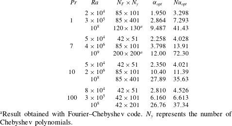
were obtained with code 2 in that reference. Grid resolutions at different
 $\mathit{Pr}$
and low, intermediate and high
 $\mathit{Ra}$
are summarized in table 1, where
 $N_{F}$
represents the number of Fourier modes and
 $N_{y}$
represents the number of grid points in the vertical direction. As will be discussed in § 4, optimal solutions are typically found at larger values of horizontal wavenumber. Therefore, for fixed
 $\mathit{Pr}$
and increasing
 $\mathit{Ra}$
, the increase in optimal wavenumber (
 ${\it\alpha}_{opt}$
) results in only a modest increase in horizontal resolution. We have also presented the optimal horizontal wavenumber in table 1 for reference with corresponding
 $\mathit{Nu}$
.
Parameters from selected simulation runs. Results are presented for various
 $\mathit{Pr}$
at low, intermediate and high
 $\mathit{Ra}$
. The spatial resolution is provided. The wavenumber at which the optimal solution is found (
 ${\it\alpha}_{opt}$
) is provided, as is the corresponding Nusselt number (
 $\mathit{Nu}_{opt}$
).

a
Result obtained with Fourier–Chebyshev code.
 $N_{y}$
represents the number of Chebyshev polynomials.
3.2. Flow map algorithm and fixed points
We now describe the flow map algorithm used to determine fixed points of this system. Let
 $X=({\it\phi},T)$
be a vector of solutions. We introduce a spatial discretization of the equations of interest (i.e. (3.1) and (2.11)) as described in § 3.1, from which we obtain a time-dependent system of ordinary differential equations,
 $$\begin{eqnarray}\frac{\text{d}X}{\text{d}t}=F(X).\end{eqnarray}$$
One way to find steady states is to directly determine fixed points
 $X$
such that
 $$\begin{eqnarray}F(X)=0.\end{eqnarray}$$
Such methods represent direct-to-steady-state methods. An alternative way of determining fixed points is to use the flow map. Let
 $X$
be any initial state and
 $X_{{\it\tau}}$
the corresponding solution at time
 ${\it\tau}$
. If
 $X$
is a fixed point, then the difference
 $$\begin{eqnarray}G_{{\it\tau}}(X)=\frac{X_{{\it\tau}}-X}{{\it\tau}}\end{eqnarray}$$
should be zero. Hence the goal is to find
 $X$
such that
 $$\begin{eqnarray}G_{{\it\tau}}(X)=0.\end{eqnarray}$$
For a small integration time
 ${\it\tau}$
, the difference
 $X_{{\it\tau}}-X$
will be small. We divide by
 ${\it\tau}$
so that
 $G_{{\it\tau}}(X)\rightarrow F(X)$
as
 ${\it\tau}\rightarrow 0$
. On the other hand, it is expected that
 $G_{{\it\tau}}(X)\rightarrow 0$
as
 ${\it\tau}\rightarrow \infty$
, assuming that
 $|X_{{\it\tau}}-X|$
is bounded. Choosing
 ${\it\tau}$
is a matter of experience for a particular problem, but it should be relatively small compared to the time scales of the modes that prevent rapid relaxation to steady state.
We have studied the effects of the flow map approach on solving a large linear system of equations
 $\text{d}X/\text{d}t=\boldsymbol{A}X-\boldsymbol{b}$
, where the eigenvalues of
 $\boldsymbol{A}$
mimic those of problems of interest, such as diffusion. The flow map acts as a preconditioner for the resulting Jacobian matrix: it can improve the condition number of the Jacobian matrix and redistribute the eigenvalues such that they cluster around the origin. These observations are consistent with previous studies (Sánchez et al.
Reference Sánchez, Net, Garcıa-Archilla and Simó2004) and indicate improvements for solving some linear systems of equations. In particular, the generalized minimum residual (GMRES) method is known to converge well when the eigenvalues of the matrix are clustered around the origin (Trefethen & Bau III Reference Trefethen and Bau III1997).
3.3. Details of the flow map algorithm
Equation (3.6) represents a large system of equations with approximately
 $N$
unknowns, where
 $N$
increases with
 $\mathit{Ra}$
. In this study
 $N\approx 10^{6}$
for the largest values of
 $\mathit{Ra}$
used. Equation (3.6) is typically solved using some variant of Newton’s method. The full version of Newton’s method can be difficult to implement and expensive to use. Difficulties include forming the full Jacobian matrix and efficiently solving the resulting matrix system. Sophisticated approaches exist to help make Newton’s method more cost-effective. These include preconditioning the Jacobian matrix, inexact Newton methods based on Krylov subspaces, and Jacobian-free methods (Knoll & Keyes Reference Knoll and Keyes2004).
In the present work, we solve (3.6) by means of a Jacobian-free Newton–Krylov method. Newton’s method results in the linear system
 $$\begin{eqnarray}\left.\frac{\text{d}G_{{\it\tau}}}{\text{d}X}\right|_{X=X_{k}}{\rm\Delta}X=-G_{{\it\tau}}|_{X=X_{k}},\end{eqnarray}$$
where
 $X_{k}$
represents the solutions at nonlinear iteration
 $k$
and
 ${\rm\Delta}X=X_{k+1}-X_{k}$
. Rather than forming the full Jacobian, a forward finite difference scheme is used to approximate the action of the Jacobian on
 ${\rm\Delta}X$
(Knoll & Keyes Reference Knoll and Keyes2004). The GMRES method is then used to solve the resulting linear system (Saad & Schultz Reference Saad and Schultz1986; Trefethen & Bau III Reference Trefethen and Bau III1997). We note that it is not necessary to form the full Jacobian (or even its approximation) because the GMRES algorithm only requires the action of a matrix on the solution. Each iteration of the GMRES method solves (3.7) with
 $$\begin{eqnarray}\left.\frac{\text{d}G_{{\it\tau}}}{\text{d}X}\right|_{X=X_{k}}{\rm\Delta}X\approx \frac{G_{{\it\tau}}(X_{k}+{\it\epsilon}{\rm\Delta}X)-G_{{\it\tau}}(X_{k})}{{\it\epsilon}},\end{eqnarray}$$
with the choice
 $$\begin{eqnarray}{\it\epsilon}=\frac{\sqrt{{\it\epsilon}_{machine}}}{\Vert {\rm\Delta}X\Vert ^{2}}\,\text{max}(X_{k}\cdot {\rm\Delta}X,\Vert {\rm\Delta}X\Vert ),\end{eqnarray}$$
where
 ${\it\epsilon}_{machine}$
is the machine tolerance and
 $\Vert \cdot \Vert$
is the
 $L_{2}$
norm. Several possibilities exist for the choice of
 ${\it\epsilon}$
(see Knoll & Keyes Reference Knoll and Keyes2004, p. 363) but the main point is that it must be small enough to get an accurate derivative in (3.8) but not so small that floating-point errors pollute the solution (Dennis & Schnabel Reference Dennis and Schnabel1996, § 5.4).
We conclude this section with a few comments and observations based on our experience with the flow map algorithm. The fact that the flow map algorithm redistributes the eigenvalues of the Jacobian matrix also has benefits when using the GMRES method to solve the linear system (3.7). To understand the latter, recall that the basis vectors for the Krylov subspace are formed from a power method, and that the power method focuses on the largest eigenvalue of the system. Since the flow map algorithm results in a larger separation between the largest eigenvalue and the other eigenvalues, the power method converges faster. Hence, a smaller Krylov subspace is required for the linear solves.
In terms of computation time, there appears to be an optimal integration time
 ${\it\tau}$
that minimizes the wall-clock time of the simulation. This optimal time is dependent upon the problem at hand. For example, increasing
 ${\it\tau}$
causes all time integrations to take longer. On the other hand, increasing
 ${\it\tau}$
allows for better preconditioning and results in a much reduced time for solving the linear system. For the current problem, we have observed that
 ${\it\tau}\approx 0.6$
results in the quickest computation time for low
 $\mathit{Ra}$
around
 $10^{5}$
. We have used
 ${\it\tau}=2$
throughout for both high and low
 $\mathit{Ra}$
. Some of the results presented herein for
 $\mathit{Pr}=1$
(
 $\mathit{Ra}\geqslant 3\times 10^{6}$
) and
 $\mathit{Pr}=7$
(
 $\mathit{Ra}\geqslant 10^{7}$
) were computed with code 2 in Waleffe et al. (Reference Waleffe, Boonkasame and Smith2015), which is based on spectral Chebyshev integration and does not use GMRES.
4. Results
In this section, we present steady solutions to the Oberbeck–Boussinesq equations that maximize heat transport. We consider Prandtl numbers
 $\mathit{Pr}$
ranging from
 $1$
to
 $100$
and note that these values roughly correspond to real fluids. For example,
 $\mathit{Pr}=7$
is often used for water, and engine oil has
 $\mathit{Pr}$
of roughly
 $100$
. In § 4.1, we explore the effects of both
 $\mathit{Pr}$
and the horizontal wavenumber
 ${\it\alpha}$
on optimal heat transport. Section 4.2 investigates the impact of
 $\mathit{Pr}$
on scaling laws, while § 4.3 discusses the coherent structures that give rise to the optimal solutions. The mean temperature profiles associated with the optimal solutions are considered in § 4.4.
4.1. Multiple local maxima and
 $\mathit{Pr}$
effects

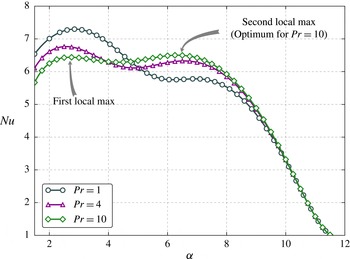
The variation of heat transport
 $\mathit{Nu}$
with wavenumber
 ${\it\alpha}$
is shown in figure 1 for
 $\mathit{Pr}=1$
,
 $\mathit{Pr}=4$
and
 $\mathit{Pr}=10$
at fixed
 $\mathit{Ra}=3\times 10^{5}$
. We note that two local maxima emerge for these three fluids. Thus, there are two scales that locally maximize heat transport. The solution corresponding to the global maximum, hereafter called the optimal solution, occurs at different length scales depending upon the fluid under consideration. For example, the global maximum occurs at a small wavenumber
 ${\it\alpha}$
for
 $\mathit{Pr}=1$
, whereas it occurs at a larger
 ${\it\alpha}$
for
 $\mathit{Pr}=10$
. We have indicated in figure 1 the ‘first’ and ‘second’ local maxima for
 $\mathit{Pr}=10$
. When we refer to the first local maximum, we have in mind the maximum that occurs at smaller wavenumber
 ${\it\alpha}$
, whereas when we refer to the second local maximum, we mean the maximum that occurs at larger wavenumber
 ${\it\alpha}$
.
Variation of
 $\mathit{Nu}$
with horizontal wavenumber
 ${\it\alpha}$
at
 $\mathit{Ra}=3\times 10^{5}$
for
 $\mathit{Pr}=1,4,10$
.

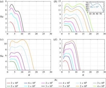
Variation of
 $\mathit{Nu}$
with horizontal wavenumber
 ${\it\alpha}$
for various
 $\mathit{Ra}$
at (a)
 $\mathit{Pr}=1$
, (b)
 $\mathit{Pr}=7$
, (c)
 $\mathit{Pr}=10$
and (d)
 $\mathit{Pr}=100$
. A legend has been provided to indicate the colours of the lines for each
 $\mathit{Ra}$
. Note that different
 $\mathit{Ra}$
are shown in different figures but that the colours for like
 $\mathit{Ra}$
are the same. The scale of
 $\mathit{Nu}$
between plots is different but the
 ${\it\alpha}$
scale is identical.

An intriguing behaviour is illuminated upon inspection of other
 $\mathit{Ra}$
and
 $\mathit{Pr}$
. As indicated in figure 2, it is not always the case that two local maxima are present. Four different scenarios are described in figure 2 for
 $\mathit{Pr}=1$
(a),
 $\mathit{Pr}=7$
(b),
 $\mathit{Pr}=10$
(c) and
 $\mathit{Pr}=100$
(d).
- Figure 2(a):
-
$\mathit{Pr}=1$
;
$2\times 10^{4}\leqslant \mathit{Ra}\leqslant 3\times 10^{5}$
. For
$\mathit{Ra}<10^{5}$
only one maximum exists. However, for
$\mathit{Ra}\geqslant 2\times 10^{5}$
we observe two local maxima. The first maximum is the optimal solution and there is no indication (at least for
$\mathit{Ra}<3\times 10^{5}$
) that the second local maximum will become the global maximum.
- Figure 2(b):
-
$\mathit{Pr}=7$
;
$5\times 10^{4}\leqslant \mathit{Ra}\leqslant 4\times 10^{6}$
. For
$\mathit{Ra}<10^{5}$
there is only one local maximum. However, for
$\mathit{Ra}\geqslant 10^{5}$
two local maxima are present. Moreover, the second local maximum is growing, and by
$\mathit{Ra}=3\times 10^{6}$
, the two local maxima are nearly identical, although they occur at different scales. In this
$\mathit{Ra}$
range, it is not clear whether the first local maximum or the second local maximum will ultimately be the optimal solution, and the issue must be settled by computing maxima at higher
$\mathit{Ra}$
. We have performed these computations, and the inset presents the
$\mathit{Nu}({\it\alpha})$
behaviour at
$\mathit{Ra}=10^{9}$
. We observe that at this
$\mathit{Ra}$
the second local maximum has receded compared to the first local maximum.
- Figure 2(c):
-
$\mathit{Pr}=10$
;
$5\times 10^{4}\leqslant \mathit{Ra}\leqslant 2\times 10^{6}$
. Yet another scenario is observed, wherein the new feature is that the second local maximum actually becomes the global maximum above a certain
$\mathit{Ra}$
. The second local maximum appears at
$\mathit{Ra}\approx 9\times 10^{4}$
and grows relative to the first local maximum. At
$\mathit{Ra}\approx 2\times 10^{5}$
, the second local maximum is equal to the first local maximum. Beyond this
$\mathit{Ra}$
, the second local maximum becomes the global maximum.
- Figure 2(d):
-
$\mathit{Pr}=100$
;
$2\times 10^{4}\leqslant \mathit{Ra}\leqslant 5\times 10^{5}$
. The large
$\mathit{Pr}=100$
case introduces a fourth type of behaviour with
$\mathit{Ra}$
, where the first local maximum vanishes for high enough
$\mathit{Ra}$
. Once again, a single local maximum is present for
$\mathit{Ra}$
below a certain value, this time
$\mathit{Ra}=8.5\times 10^{4}$
. A second local maximum appears at
$\mathit{Ra}=8.5\times 10^{4}$
and begins to grow relative to the first local maximum. By
$\mathit{Ra}=10^{5}$
, the first and second local maxima are equal. Interestingly, by
$\mathit{Ra}=2\times 10^{5}$
the first local maximum has vanished and the second local maximum is the global maximum.













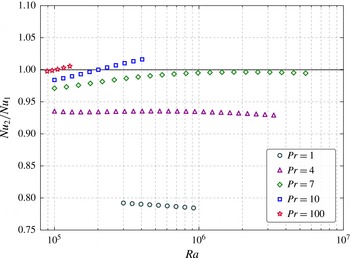
Ratio of local maxima as a function of
 $\mathit{Ra}$
for various
 $\mathit{Pr}$
.

For ease of discussion below, we use the term ‘coexistence interval’ to refer to the
 $\mathit{Ra}$
interval in which two local maxima are present, recognizing that the interval changes with
 $\mathit{Pr}$
.
Figure 3 summarizes the different scenarios we observed in the Prandtl-number range
 $1\leqslant \mathit{Pr}\leqslant 100$
, for Rayleigh numbers
 $\mathit{Ra}<10^{7}$
. Figure 3 shows the ratio of the second local maximum to the first local maximum
 $\mathit{Nu}_{2}/\mathit{Nu}_{1}$
as a function of
 $\mathit{Ra}$
. For
 $\mathit{Pr}=1$
,
 $\mathit{Pr}=4$
and
 $\mathit{Pr}=7$
, the second local maximum does not overtake the first maximum, whereas for
 $\mathit{Pr}=10$
and
 $\mathit{Pr}=100$
the second maximum eventually becomes the global maximum. For
 $\mathit{Pr}=7$
, the two maxima are almost equal, with the second local maximum becoming 99.6 % of the first local maximum at
 $\mathit{Ra}\approx 2\times 10^{6}$
before slowly dropping off. We also note that the coexistence region of the two maxima depends heavily on
 $\mathit{Pr}$
. This is most clearly observed for the
 $\mathit{Pr}=100$
case, in which the two maxima coexist only for a very small interval of
 $\mathit{Ra}$
. For
 $\mathit{Pr}=4$
,
 $\mathit{Pr}=7$
and
 $\mathit{Pr}=10$
, we did not observe termination of the coexistence region. However, for
 $\mathit{Pr}=1$
and
 $\mathit{Pr}=100$
the coexistence region was found to be finite, with the second (first) maximum disappearing for
 $\mathit{Pr}=1$
(
 $\mathit{Pr}=100$
). Figure 3 implies the existence of two different parametric regions for optimal heat transport roughly partitioned by
 $\mathit{Pr}=7$
. For
 $\mathit{Pr}>7$
, the second local maximum overtakes the first local maximum to become the optimal solution and appears to remain the optimal solution. Since the second local maximum occurs at larger
 ${\it\alpha}$
, our calculations suggest that optimal solutions occur at relatively smaller scales for fluids with
 $\mathit{Pr}>7$
at high enough
 $\mathit{Ra}$
. Conversely, for
 $\mathit{Pr}\lesssim 7$
and
 $\mathit{Ra}<6\times 10^{6}$
, our data suggest that the second local maximum does not overtake the first local maximum, and therefore the first local maximum remains the optimal solution. Thus, for fluids with
 $\mathit{Pr}\lesssim 7$
and the range of
 $\mathit{Ra}$
considered herein, optimal solutions occur at the larger of the two length scales. The
 $\mathit{Pr}$
dependence is significant in determining the flow structure that leads to optimal solutions.
4.2. Scaling laws and impact of
$\mathit{Pr}$

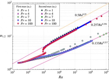
Figures 4 and 5 present log–log plots of optimal
 $\mathit{Nu}$
and optimal
 ${\it\alpha}$
with
 $\mathit{Ra}$
. In figure 4 we observe the dependence of the optimal
 $\mathit{Nu}$
on
 $\mathit{Ra}$
in the form
 $\mathit{Nu}\propto \mathit{Ra}^{{\it\gamma}}$
for
 $\mathit{Ra}>10^{5}$
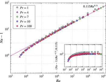
. The scaling law of
 $\mathit{Nu}=0.115\mathit{Ra}^{0.31}$
was determined for
 $\mathit{Pr}=7$
in Waleffe et al. (Reference Waleffe, Boonkasame and Smith2015), and is shown by the dashed line in figure 4 for comparison. This scaling was obtained from data in the range
 $10^{7}\leqslant \mathit{Ra}\leqslant 10^{9}$
. We observe that there is very little variation from this scaling with
 $\mathit{Pr}$
although the prefactor for
 $\mathit{Pr}=1$
is higher. The inset in figure 4 shows a compensated version of the
 $\mathit{Nu}$
scaling with
 $\mathit{Ra}$
for the optimal solutions. This compensated plot confirms our initial observations that there is very little variation in the scaling laws other than minor differences in the prefactor, with the
 $\mathit{Pr}=1$
prefactor being the largest.
Optimal
 $\mathit{Nu}$
versus
 $\mathit{Ra}$
; global optimal data are shown and may correspond to a distinct wavenumber.

Maximal
 ${\it\alpha}$
versus
 $\mathit{Ra}$
; open markers indicate the first maximum and filled markers indicate the second maximum; the upper dash-dotted line represents the upper bound from linear stability theory.

Figure 5 shows the dependence of the two maximal wavenumbers
 ${\it\alpha}_{1,2}$
on the Rayleigh number
 $\mathit{Ra}$
. We begin our discussion by focusing on the open markers in figure 5 (first maximum). For
 $\mathit{Pr}=100$
, the first local maximum
 ${\it\alpha}_{1}$
vanishes after
 $\mathit{Ra}=1.3\times 10^{5}$
, and hence a clear scaling of
 ${\it\alpha}_{1}$
with
 $\mathit{Ra}$
cannot be determined. However, for the other
 $\mathit{Pr}$
considered in this work, a scaling regime appears. The scaling of
 ${\it\alpha}_{1}$
determined in Waleffe et al. (Reference Waleffe, Boonkasame and Smith2015) for
 $\mathit{Pr}=7$
is shown by the dashed line:
 ${\it\alpha}_{1}=0.133\mathit{Ra}^{0.217}$
. Once again, the scaling shows almost no change with
 $\mathit{Pr}$
. For
 $\mathit{Pr}=1$
the power law of the scaling appears consistent with the other
 $\mathit{Pr}$
, although it is likely that the prefactor is larger. We note that, for
 $\mathit{Ra}<10^{5}$
, the
 $\mathit{Ra}$
dependence of
 ${\it\alpha}_{1}$
exhibits some wobbles, conjectured to be linked to the appearance or disappearance of coiling arms emanating from the central temperature plume of the optimal steady solutions (Waleffe et al.
Reference Waleffe, Boonkasame and Smith2015).
Next we turn attention to the closed markers in figure 5 corresponding to the second maximum with wavenumber
 ${\it\alpha}_{2}$
. A scaling regime emerges at
 $\mathit{Ra}\approx 10^{6}$
, and the scaling regime for these solutions is more complete because all fluids considered in this work exhibited a second local maximum in vertical heat transport that persisted for several decades of
 $\mathit{Ra}$
. For
 $\mathit{Pr}=7$
we find
 ${\it\alpha}_{2}\approx 0.257\mathit{Ra}^{0.256}$
with the current range of
 $\mathit{Ra}$
sampled by our data. It can be shown from linear stability theory (
 $\mathit{Nu}=1$
) that the upper wavenumber limit for marginal stability
 ${\it\alpha}_{u}$
scales as
 ${\it\alpha}_{u}\sim 0.5\mathit{Ra}^{1/4}$
for large
 $\mathit{Ra}$
. This scaling is marked in the dash-dotted line in figure 5. The
 $\mathit{Nu}$
value drops to 1 as
 ${\it\alpha}$
approaches
 ${\it\alpha}_{u}$
from below and there is no convective steady state for
 ${\it\alpha}>{\it\alpha}_{u}$
(see also figure 2). We expect that data at higher
 $\mathit{Ra}$
would reduce the best-fitting
 ${\it\alpha}_{2}$
to be at or below
 ${\it\alpha}_{2}\sim \mathit{Ra}^{0.25}$
.
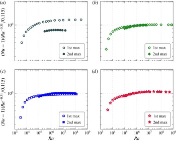
Figure 6 presents
 $\mathit{Nu}$
compensated by
 $0.115\mathit{Ra}^{0.31}$
, which is the best least-squares fit scaling of
 $\mathit{Nu}$
at
 $\mathit{Pr}=7$
observed in figure 4. In particular, we consider the
 $\mathit{Nu}$
versus
 $\mathit{Ra}$
scaling at various
 $\mathit{Pr}$
, and for each local maximum of
 $\mathit{Nu}$
(first and second local maxima). We observe that the
 $\mathit{Nu}(\mathit{Ra})$
scaling laws that result from tracking the first or second local maxima are not very different. The most obvious discrepancy in
 $\mathit{Nu}$
between the first and second local maxima occurs for
 $\mathit{Pr}=1$
. However, the compensated plots are both flat over their respective
 $\mathit{Ra}$
ranges. This indicates that the scaling exponent
 ${\it\gamma}=0.31$
is observed for both types of solutions at
 $\mathit{Pr}=1$
. The fact that the scaling of the optimal solution at
 $\mathit{Pr}=1$
is greater than unity can be attributed to a different prefactor in the scaling law (greater than
 $0.115$
). Similarly, the solution at the second local maximum has a prefactor less than
 $0.115$
. At
 $\mathit{Pr}=7$
and
 $\mathit{Pr}=10$
there is almost no discernible difference in the scaling laws between to the two types of solutions. When
 $\mathit{Pr}=100$
the optimal solution also closely follows the scaling shown in figure 4.
 $\mathit{Nu}$
compensated by
 $0.115\mathit{Ra}^{0.31}$
for various
 $\mathit{Pr}$
(1 (a), 7 (b), 10 (c), 100 (d)). Open markers: solutions from the first maximum. Filled markers: solutions from the second maximum. Optimal solutions occur when one curve is above the other curve.

4.3. Coherent structures and optimal heat transport
Sections 4.1 and 4.2 showed that the
 $\mathit{Nu}$
-maximizing wavenumbers are larger than the wavenumber
 ${\it\alpha}=1.5585$
corresponding to the onset of convection (the primary wavenumber). Thus the maximizing solutions have smaller horizontal scales than their non-optimal counterparts in the primary box. Here we compare the details of the optimal and non-optimal coherent structures.
Temperature contours at
 $\mathit{Ra}=10^{5}$
and
 $\mathit{Pr}=100$
: (a) the primary solution (
 ${\it\alpha}=1.5585$
,
 $\mathit{Nu}=4.429$
), (b) contours at the first local maximum (
 ${\it\alpha}=3.0$
,
 $\mathit{Nu}=4.819$
), and (c) contours at the second local maximum (
 ${\it\alpha}=4.3$
,
 $\mathit{Nu}=4.821$
). Note that the second local maximum is the optimal solution at the
 $\mathit{Ra}$
considered.

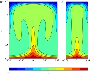
Temperature contours at
 $\mathit{Pr}=10$
and
 $\mathit{Ra}=2\times 10^{6}$
: (a) contours for the first local maximum of
 $\mathit{Nu}$
occur at
 ${\it\alpha}=3.35$
and
 $\mathit{Nu}=11.009$
; (b) contours corresponding to optimal
 $\mathit{Nu}$
occur at
 ${\it\alpha}=10.45$
and
 $\mathit{Nu}=11.391$
.

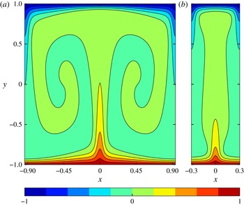
In figure 7, contours of temperature in the channel are plotted for
 $\mathit{Pr}=100$
at
 $\mathit{Ra}=10^{5}$
. Figure 7(a) is the non-optimal temperature in the primary box with wavenumber
 ${\it\alpha}=1.5585$
. The main features are the thick horizontal temperature arms emanating from the main plume that roll up with increasing
 $\mathit{Ra}$
. By contrast, the plumes in figure 7(b,c) maximize vertical heat transport and exhibit much less, if any, horizontal structure. In fact, the thermal plume corresponding to the optimal solution (figure 7
c) does not have any spiral arms or lobes; the heat transport is almost exclusively straight up and down in the vertical direction. Similar results are shown in figure 8 for
 $\mathit{Pr}=10$
at
 $\mathit{Ra}=2\times 10^{6}$
. Again, the optimal temperature structure is a single plume without significant horizontal structure (figure 8
b; second local maximum), while the non-optimal plume (figure 8
a; first local maximum) has coiling arms emanating from the central plume. Figures 7 and 8 show representative optimal solutions in fluids with
 $\mathit{Pr}>7$
at large enough
 $\mathit{Ra}$
, for which the optimal solution occurs at small scales (large
 ${\it\alpha}$
; the second maximum).
However, as shown in figure 9, the temperature structure of optimal solutions for
 $\mathit{Pr}\lesssim 7$
seems to contradict the simple optimal structure seen for
 $\mathit{Pr}>7$
. The contours in figure 9 are for
 $\mathit{Pr}=1$
at
 $\mathit{Ra}=5\times 10^{5}$
, with optimal solution in figure 9(a) (
 ${\it\alpha}=3.7$
; first maximum), and non-optimal solution in figure 9(b) (
 ${\it\alpha}=8.1$
; second maximum). As expected, horizontal structure is prohibited by the large-
 ${\it\alpha}$
maximum, but in this case there is relatively weak vertical heat transport associated with the central plume. The smaller wavenumber (larger horizontal scale) allows for downdraughts to the left and right of centre, which in turn allows for more vigorous updraught of heat in the centre, and thus an overall larger vertical heat transport. Contours of the optimal vertical velocity (not shown here) confirm that the vertical velocity is largest in the middle of the channel.
Thus, depending on the
 $\mathit{Pr}$
and
 $\mathit{Ra}$
numbers, there is a delicate balance determining whether or not the optimal solution will have horizontal structure in the form of coiling arms emanating from the central plume. For
 $\mathit{Pr}>7$
at large enough
 $\mathit{Ra}$
, the optimal solution is the ‘second maximum’ corresponding to small horizontal scale that does not admit significant horizontal structure. In this case, top to bottom heat transport through the central plume is the most efficient conduit for overall vertical heat transport. For
 $\mathit{Pr}\lesssim 7$
, the optimal solution is the ‘first maximum’ corresponding to a larger horizontal scale, wherein the largest overall vertical heat transport is achieved through a vigorous central updraught accompanied by adjacent downdraughts.
(a) Temperature contours at
 $\mathit{Pr}=1$
and
 $\mathit{Ra}=3\times 10^{5}$
corresponding to optimal
 $\mathit{Nu}$
occur at
 ${\it\alpha}=3.7$
and
 $\mathit{Nu}=7.058$
. (b) Temperature contours for the second local maximum of
 $\mathit{Nu}$
occur at
 ${\it\alpha}=8.1$
and
 $\mathit{Nu}=5.473$
.

We close this subsection with a visualization of the optimizing solution at
 $\mathit{Ra}=10^{8}$
for
 $\mathit{Pr}=1$
,
 $\mathit{Pr}=7$
and
 $\mathit{Pr}=10$
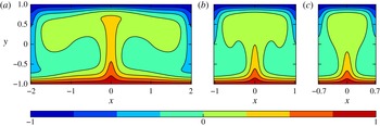
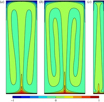
(figures 10–12). Figure 10 shows the morphology of the optimal temperature contours at each
 $\mathit{Pr}$
considered. We note that the optimal solutions at
 $\mathit{Pr}=1$
and
 $\mathit{Pr}=7$
are found at larger scales. Despite this, the temperature contours still exhibit considerable differences. The optimal contours at
 $\mathit{Pr}=1$
have droopy arms, whereas the optimal contours at
 $\mathit{Pr}=7$
display a distinct coiling pattern. Very little structure is observed in the optimal solution at
 $\mathit{Pr}=10$
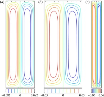
. In fact, the arms of the temperature contours are almost entirely invisible. Figure 11 shows corresponding streamlines at each
 $\mathit{Pr}$
and
 $\mathit{Ra}=10^{8}$
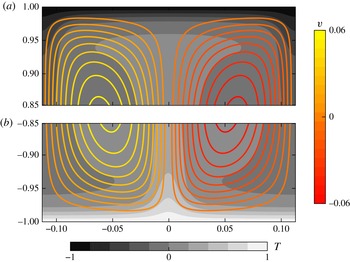
. Figure 12(a,b) shows the top and bottom portions, respectively, of the optimal temperature field with streamlines superposed at
 $\mathit{Pr}=10$
. A main feature to note is that the streamlines deeply penetrate the thermal boundary layer, which has thickness
 ${\it\delta}_{T}\approx H/(2\mathit{Nu})=0.0281$
. We remark that Hassanzadeh, Chini & Doering (Reference Hassanzadeh, Chini and Doering2014) found optimal solutions for a related problem in which the class of solutions was expanded to include all divergence-free velocity fields with fixed enstrophy and free-slip boundary conditions. The aspect ratio in that work was found to scale as
 $\mathit{Ra}^{1/4}$
, as in the present work. One notable difference is that we do not observe the formation of a recirculation region near the top of the channel.
Results for
 $\mathit{Ra}=10^{8}$
. Temperature contours for the optimal solution at (a)
 $\mathit{Pr}=1$
with
 ${\it\alpha}=9.5$
and
 $\mathit{Nu}=41.49$
, (b)
 $\mathit{Pr}=7$
with
 ${\it\alpha}=7.23$
and
 $\mathit{Nu}=35.95$
and (c)
 $\mathit{Pr}=10$
with
 ${\it\alpha}=27.86$
and
 $\mathit{Nu}=35.63$
. As usual
 $y\in [-1,1]$
and
 $x\in [-{\rm\pi}/{\it\alpha},{\rm\pi}/{\it\alpha}]$
.

Results for
 $\mathit{Ra}=10^{8}$
. Streamlines for the optimal solution at
 $\mathit{Pr}=1$
with (a)
 ${\it\alpha}=9.5$
and
 $\mathit{Nu}=41.49$
, (b)
 $\mathit{Pr}=7$
with
 ${\it\alpha}=7.23$
and
 $\mathit{Nu}=35.95$
and (c)
 $\mathit{Pr}=10$
with
 ${\it\alpha}=27.86$
and
 $\mathit{Nu}=35.63$
. As usual
 $y\in [-1,1]$
and
 $x\in [-{\rm\pi}/{\it\alpha},{\rm\pi}/{\it\alpha}]$
.

Streamlines of the optimal solution at
 $\mathit{Pr}=10$
and
 $\mathit{Ra}=10^{8}$
near the top (a) and bottom (b) superposed on contours of temperature where
 $x\in [-{\rm\pi}/{\it\alpha},{\rm\pi}/{\it\alpha}]$
and
 ${\it\alpha}=27.86$
. The thermal boundary layer thickness is
 ${\it\delta}_{T}\approx H/(2\mathit{Nu})=0.0281$
.

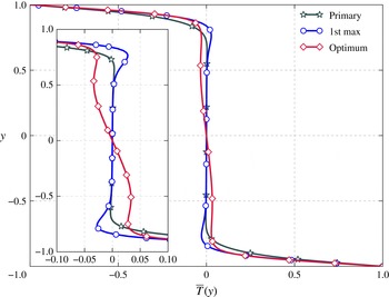
Horizontally averaged temperature profiles for
 $\mathit{Pr}=10$
at
 $\mathit{Ra}=2\times 10^{6}$
.

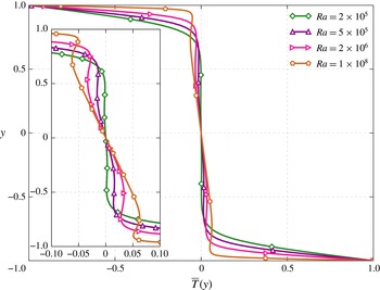
Horizontally averaged optimal temperature profiles at
 $\mathit{Pr}=10$
for
 $2\times 10^{5}\leqslant \mathit{Ra}\leqslant 10^{8}$
.

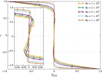
Horizontally averaged optimal temperature profiles at
 $\mathit{Pr}=1$
for
 $10^{5}\leqslant \mathit{Ra}\leqslant 10^{8}$
.

4.4. Mean temperature profiles and
$\mathit{Nu}(\mathit{Pr})$

We now consider mean temperature profiles of the optimal solutions introduced in § 4.3. Figures 13 and 14 present mean temperature profiles at
 $\mathit{Pr}=10$
. First, in figure 13 we compare mean temperature profiles at
 $\mathit{Ra}=2\times 10^{6}$
of the primary solution, the optimal solution and the solution that gives the first maximum. The primary solution is nearly marginally stable, possessing a nearly isothermal region through the core of the channel. However, a very slight stable stratification of the primary solution can be observed in the inset of figure 13 just above
 $y=0.5$
. The solution corresponding to the first maximum is marginally stable in the centre of the channel but exhibits stably stratified transition regions between the centre and the unstably stratified boundary layers. The optimal solution, on the other hand, is unstably stratified in the centre of the channel, but maintains the stably stratified transition regions and the unstable boundary layers. We note that non-monotonic temperature profiles have been considered in the infinite
 $\mathit{Pr}$
case (Doering, Otto & Reznikoff Reference Doering, Otto and Reznikoff2006). Interestingly, each solution presented in figure 13 is close to the marginally stable configuration constructed by Malkus (Reference Malkus1954) and resulting in the prediction of
 $\mathit{Nu}\sim \mathit{Ra}^{1/3}$
.
As shown in figure 4, the scaling of the optimal solution
 $\mathit{Nu}\sim \mathit{Ra}^{0.31}$
is less than
 $\mathit{Nu}\sim \mathit{Ra}^{1/3}$
, which might be attributed to small departures from marginal stability. Figure 14 shows optimal mean temperature profiles at
 $\mathit{Pr}=10$
for
 $2\times 10^{5}\leqslant \mathit{Ra}\leqslant 10^{8}$
. Each of these profiles exhibits unstable stratification in the bulk and in the boundary layers, but still possesses the stably stratified transition regions. Perhaps surprisingly, the optimal solutions become more unstably stratified in the bulk as
 $\mathit{Ra}$
increases, and thus departure from marginal stability seems to grow. The latter is related to the single updraught nature of the optimal solutions, which have increasing horizontal wavenumber and diminishing horizontal structure; there are no significant horizontal arms or coils to bring colder fluid beneath warmer fluid.
A different trend is observed for
 $\mathit{Pr}\lesssim 7$
, as illustrated in figure 15, showing horizontally averaged optimal temperature profiles at
 $\mathit{Pr}=1$
for
 $10^{5}\leqslant \mathit{Ra}\leqslant 10^{8}$
. At first glance, these profiles all appear to be marginally stable. The inset in figure 15 shows that this observation is not quite the entire story. Indeed, near the centre of the channel, the profiles are nearly marginally stable, with a tendency towards stable stratification, especially at lower
 $\mathit{Ra}$
. Stably stratified transition regions between the centre of the channel and the boundary layers are once again present. The mean stable stratification is linked to the two downdraughts on either side of the central updraught, which bring colder fluid underneath warmer fluid in a stable configuration.
Figures 13–15 suggest that for
 $\mathit{Pr}\lesssim 7$
optimal solutions have a stably stratified bulk region whereas the optimal solutions for
 $\mathit{Pr}>7$
have an unstably stratified bulk region. Figure 16 provides more evidence of this emerging picture, presenting optimal solutions at
 $\mathit{Ra}=5\times 10^{5}$
for
 $\mathit{Pr}=1,4,7,10,100$
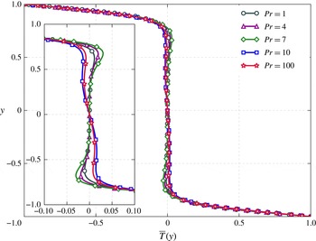
. Indeed, the optimal mean temperature profiles for
 $\mathit{Pr}=1,4,7$
are stably stratified near the middle of the channel, while those for
 $\mathit{Pr}=10$
and
 $\mathit{Pr}=100$
are unstably stratified. The stably stratified transition regions between the middle of the channel and the boundary layers are present at all
 $\mathit{Pr}$
. We summarize the three regions observed in the optimal temperature profiles as follows:
-
(a) The temperature boundary conditions produce unstable boundary layers.
-
(b) The central region of the channel may be stably stratified (
$\mathit{Pr}\lesssim 7$
) or unstably stratified (
$\mathit{Pr}>7$
). -
(c) The transition regions between the channel centre and the boundary layers were always observed to be stably stratified in the optimal transport solutions.


Horizontally averaged optimal temperature profiles at
 $\mathit{Ra}=5\times 10^{5}$
for
 $\mathit{Pr}=1$
, 4, 7, 10 and 100.

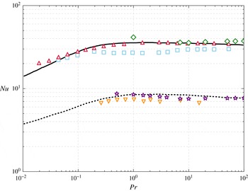
Comparison of 2D optimal solutions to the GL theory and to turbulent solutions. The black dashed and solid lines represent the GL theory at
 $\mathit{Ra}=5\times 10^{5}$
and
 $\mathit{Ra}=10^{8}$
, respectively. The gold downward-pointing triangles and red upward-pointing triangles represent 3D turbulent data at
 $\mathit{Ra}=5\times 10^{5}$
(Verzicco & Camussi Reference Verzicco and Camussi1999) and
 $\mathit{Ra}=10^{8}$
(van der Poel, Stevens & Lohse Reference van der Poel, Stevens and Lohse2013), respectively. The 2D turbulent data at
 $\mathit{Ra}=10^{8}$
are shown in blue squares (van der Poel et al.
Reference van der Poel, Stevens and Lohse2013). Finally, the purple stars present the 2D optimal solutions at
 $\mathit{Ra}=5\times 10^{5}$
, and the green diamonds present the 2D optimal solutions at
 $\mathit{Ra}=10^{8}$
, which were both computed in this work.

Finally, we compare the 2D optimal solutions found in the present work to the GL theory of turbulent convection (Grossmann & Lohse Reference Grossmann and Lohse2000) and to fully 3D numerical simulations (Verzicco & Camussi Reference Verzicco and Camussi1999; van der Poel et al.
Reference van der Poel, Stevens and Lohse2013). In figure 17 we show the variation of
 $\mathit{Nu}$
with
 $\mathit{Pr}$
for
 $0.5\leqslant \mathit{Pr}\leqslant 100$
at
 $\mathit{Ra}=5\times 10^{5}$
and at
 $\mathit{Ra}=10^{8}$
. The work presented here corresponds to regions
 $\text{I}_{u}$
and
 $\text{II}_{u}$
as well as the beginning of region
 $\text{IV}_{u}$
in the
 $\mathit{Pr}{-}\mathit{Ra}$
phase diagram of the GL theory (Grossmann & Lohse Reference Grossmann and Lohse2001). In each of these regions the thermal boundary layer is nested within the viscous boundary layer. We remark that the 2D optimal solutions are in agreement with both the GL theory as well as the 3D turbulent solutions. This intriguing observation begs the question: Do the 2D steady solutions computed in the present work play a role in the dynamics of 3D turbulent convection? Preliminary evidence suggests that 2D solutions may be relevant in 3D turbulent convection. For example, at high
 $\mathit{Ra}$
, 2D sheet-like structures appear (van der Poel et al.
Reference van der Poel, Ostilla-Mónico, Donners and Verzicco2015). For future consideration of the possible connection, one must consider aspect-ratio effects as well as the difference in dimensionality (2D versus 3D). We note that van der Poel et al. (Reference van der Poel, Stevens and Lohse2013) have catalogued differences between 2D and 3D solutions. Moreover, the theoretical Rayleigh–Bénard problem has an essentially infinite aspect ratio, whereas the aspect-ratio-dependent parameters in the GL theory have been fitted to experiments with aspect ratio
 ${\it\Gamma}\leqslant 1$
. The turbulent simulations of Verzicco & Camussi (Reference Verzicco and Camussi1999) were performed in a cylindrical cell with
 ${\it\Gamma}=1$
. There is evidence, however, that aspect-ratio dependence may be weak (Ahlers et al.
Reference Ahlers, Grossmann and Lohse2009), although recent results (Bailon-Cuba, Emran & Schumacher Reference Bailon-Cuba, Emran and Schumacher2010) indicate that, at least for small aspect ratio, there is indeed a
 $\mathit{Nu}$
dependence on the aspect ratio. On the other hand, the sensitivity of
 $\mathit{Nu}$
to the large-scale circulation arising in finite-aspect-ratio configurations remains an open issue (Ahlers et al.
Reference Ahlers, Grossmann and Lohse2009). We note that the large-scale circulation may account for significant discrepancies between 2D and 3D flows (van der Poel et al.
Reference van der Poel, Stevens and Lohse2013).
5. Conclusions
Optimal transport solutions for 2D Rayleigh–Bénard convection have been computed for
 $\mathit{Ra}$
up to
 $10^{9}$
for
 $\mathit{Pr}\geqslant 1$
. This work is an extension to that performed by Waleffe et al. (Reference Waleffe, Boonkasame and Smith2015) at
 $\mathit{Pr}=7$
. Most of the solutions in the present work have been found using a flow map algorithm in conjunction with a Jacobian-free Newton–Krylov solver to find steady solutions to the Oberbeck–Boussinesq equations. Some of the high-
 $\mathit{Ra}$
,
 $\mathit{Pr}=1$
and
 $\mathit{Pr}=7$
solutions were computed with code 2 in Waleffe et al. (Reference Waleffe, Boonkasame and Smith2015). An optimal solution at a given
 $\mathit{Ra}$
and
 $\mathit{Pr}$
represents the steady solution that maximizes heat transport among all horizontal wavenumbers. One goal is to make contact with rigorous upper-bound theory (Howard Reference Howard1963; Busse Reference Busse1969; Doering & Constantin Reference Doering and Constantin1996) by computing optimal solutions constrained exactly by the Oberbeck–Boussinesq equations. Another intention is to compare scaling laws derived from experiments (Niemela et al.
Reference Niemela, Skrbek, Sreenivasan and Donnelly2000; He et al.
Reference He, Funfschilling, Bodenschatz and Ahlers2012a
) and computational studies (Amati et al.
Reference Amati, Koal, Massaioli, Sreenivasan and Verzicco2005) of turbulent Rayleigh–Bénard convection with our optimal solutions in the spirit of Malkus’s original idea that turbulence maximizes heat transport subject to some marginal stability constraints (Malkus Reference Malkus1954). A significant portion of this work is aimed at exploring the effect of
 $\mathit{Pr}$
on scaling laws and optimal solutions.
We have considered
 $\mathit{Pr}=1,4,7,10,100$
, and our results indicate that there is little or no variation of scaling of
 $\mathit{Nu}$
with
 $\mathit{Pr}$
(for the parameter ranges considered). This is consistent with studies in turbulent Rayleigh–Bénard convection, which report that
 $\mathit{Nu}(\mathit{Pr})$
is relatively constant for
 $\mathit{Pr}\gtrsim 1$
(see Ahlers et al.
Reference Ahlers, Grossmann and Lohse2009, figure 5). The optimal solutions exhibit a scaling of the form
 $\mathit{Nu}\sim \mathit{Ra}^{0.31}$
, which is in agreement with that found by Waleffe et al. (Reference Waleffe, Boonkasame and Smith2015). Moreover, horizontally averaged profiles of the temperature field are close to a marginally stable profile, roughly consistent with the prediction by Malkus (Reference Malkus1954), leading to
 $\mathit{Nu}\sim \mathit{Ra}^{1/3}$
. However, the lack of
 $\mathit{Pr}$
dependence for scaling relations is not the entire story. Indeed,
 $\mathit{Pr}$
is shown to have a significant impact on the scale of the optimal solution. When considering the variation of
 $\mathit{Nu}$
with
 ${\it\alpha}$
, we observe that, above a certain
 $\mathit{Ra}$
, two local maxima exist: one at a smaller scale and the other at a larger scale. There are two regions partitioned by
 $\mathit{Pr}\approx 7$
: for
 $\mathit{Pr}>7$
optimal transport solutions occur at smaller scales; and for
 $\mathit{Pr}\lesssim 7$
optimal transport solutions occur at larger scales.
One might expect optimal heat transport to be realized by direct ‘wall-to-wall’ transport of hot and cold fluid in narrow plumes with little horizontal structure and no returning downdraughts of hot fluid and updraughts of cold fluid. Inspection of the optimizing solutions reveals that this structure is associated with the ‘second maximum’ at small scales, and optimizes heat transport for
 $\mathit{Pr}>7$
at large enough
 $\mathit{Ra}$
. For
 $\mathit{Pr}\lesssim 7$
, the optimal heat transport occurs at the ‘first maximum’, and is associated with a larger horizontal scale. In this case, the vigorous central updraught is accompanied by adjacent left/right downdraughts, leading to a slightly stable interior mean temperature profile. Evidently, this is another way to minimize the thickness of the thermal boundary layer to maximize transport. Alternatively, with free-slip boundary conditions and an expanded class of velocity fields, optimal transport solutions were found to exhibit recirculation near the top of the channel (Hassanzadeh et al.
Reference Hassanzadeh, Chini and Doering2014). Thus there is a delicate balance when optimizing over all possible velocity fields: the velocity must be strong enough to efficiently transport heat vertically, but not so strong that downdraughts of heat overcompensate for the vertical transport. It is unclear why
 $\mathit{Pr}\approx 7$
should be the demarcation between smaller-scale optima consisting of a central updraught only, and larger-scale optima admitting some horizontal structure (downdraughts adjacent to the central updraught).
An obvious extension of the present work is to consider a wider range of
 $\mathit{Pr}$
and
 $\mathit{Ra}$
numbers, and in particular
 $\mathit{Pr}<1$
. Stricter spatial and temporal resolutions will be necessary, requiring algorithmic modifications, including possibly code parallelization. Another direction of our future work is understanding the connections between the optimal steady solutions and turbulent flows. It has been conjectured that such unstable solutions actually control the dynamics of turbulent flows (Waleffe Reference Waleffe2009), and the close agreement between the
 $\mathit{Nu}(\mathit{Ra})$
data for optimum 2D solutions and 3D turbulent data is most intriguing. Is it possible to detect the signature of the optimal solutions within the turbulence data? One step in this direction involves performing a fully resolved simulation at high
 $\mathit{Ra}$
and collecting local snapshots of the fields at times and locations where the Nusselt number achieves its maximal values in order to ‘educe’ a characteristic optimum transport structure (Stretch Reference Stretch1990). These snapshots can be compared to the coherent structures educed through other flow decompositions (e.g., Smith, Moehlis & Holmes Reference Smith, Moehlis and Holmes2005; Schmid Reference Schmid2010). Thus one may begin to explore statistics such as how often the optimal structures are sampled by the turbulent flow. We remark that studies based on DNS at very large aspect ratio have reported persistence of large-scale mean patterns in Rayleigh–Bénard convection even at large
 $\mathit{Ra}$
(Emran & Schumacher Reference Emran and Schumacher2015). Moreover, the proper orthogonal decomposition of Rayleigh–Bénard DNS data was employed by Bailon-Cuba et al. (Reference Bailon-Cuba, Emran and Schumacher2010) in exploring the aspect-ratio dependence of heat transport. They observed that large-scale structures are always present. Such conclusions are intriguing in light of the present work in that they point towards fundamental structures governing turbulent convection. More sophisticated analyses of the state space and the role of the stable and unstable manifolds of the optimum solutions should be easier to perform than in 3D shear flows (Gibson, Halcrow & Cvitanović Reference Gibson, Halcrow and Cvitanović2008). We hope that such investigations will be the subject of forthcoming publications.
Acknowledgements
The authors would like to thank A. Boonkasame (University of Wisconsin-Madison), G. Chini (University of New Hampshire), C. Doering (University of Michigan), D. Goluskin (University of Michigan) and A. Souza (University of Michigan) for insightful discussions and suggestions. This work was partially supported by DMS-1147523 (D.S.) and DMS-1008396 (L.M.S.).
Appendix A. Boundary conditions and time integration
A.1. Time integration
We now apply the
 $(3,4,3)$
IMEX-RK method developed by Ascher et al. (Reference Ascher, Ruuth and Wetton1995) to the Rayleigh–Bénard problem governed by (3.1) and (2.11). We rewrite the equations concisely as
 $$\begin{eqnarray}\displaystyle & \displaystyle \frac{\partial {\it\phi}}{\partial t}+\frac{\partial }{\partial x}\mathscr{N}_{{\it\phi}}={\it\nu}_{\star }{\rm\nabla}^{2}{\it\phi}+\frac{\partial ^{2}T}{\partial x^{2}}, & \displaystyle\end{eqnarray}$$
 $$\begin{eqnarray}\displaystyle & \displaystyle \frac{\partial T}{\partial t}+\mathscr{N}_{T}={\it\kappa}_{\star }{\rm\nabla}^{2}T, & \displaystyle\end{eqnarray}$$
 $$\begin{eqnarray}\displaystyle & \displaystyle \mathscr{N}_{{\it\phi}}=\mathscr{N}_{{\it\phi}}({\it\phi},u,v)=u{\it\phi}-v{\rm\nabla}^{2}u, & \displaystyle\end{eqnarray}$$
 $$\begin{eqnarray}\displaystyle & \displaystyle \mathscr{N}_{T}=\mathscr{N}_{T}(T,u,v)=\boldsymbol{u}\boldsymbol{\cdot }\boldsymbol{{\rm\nabla}}T. & \displaystyle\end{eqnarray}$$
 ${\it\phi}^{n}$
the field at the current time step. To evolve
 ${\it\phi}$
to step
 $n+1$
we have
 $$\begin{eqnarray}{\it\phi}^{n+1}={\it\phi}^{n}+{\rm\Delta}t\mathop{\sum }_{j=1}^{3}b^{j}(K_{{\it\phi}}^{j}+\widehat{K}_{{\it\phi}}^{j+1}),\end{eqnarray}$$
where
 $$\begin{eqnarray}\displaystyle & \displaystyle K_{{\it\phi}}^{j}={\it\nu}_{\star }{\rm\nabla}^{2}{\it\phi}^{i}, & \displaystyle\end{eqnarray}$$
 $$\begin{eqnarray}\displaystyle & \displaystyle \widehat{K}_{{\it\phi}}^{1}=-\frac{\partial }{\partial x}\mathscr{N}_{{\it\phi}}^{n-1}+\frac{\partial ^{2}}{\partial x^{2}}T^{n-1}, & \displaystyle\end{eqnarray}$$
 $$\begin{eqnarray}\displaystyle & \displaystyle \widehat{K}_{{\it\phi}}^{i}=-\frac{\partial }{\partial x}\mathscr{N}_{{\it\phi}}^{i-1}+\frac{\partial ^{2}}{\partial x^{2}}T^{i-1},\quad i\neq 1. & \displaystyle\end{eqnarray}$$
 $i$
,
 ${\it\phi}$
is given by
 $$\begin{eqnarray}(1-a^{ii}{\rm\Delta}t{\it\nu}_{\star }{\rm\nabla}^{2}){\it\phi}^{i}={\it\phi}^{n}+{\rm\Delta}t\left[\mathop{\sum }_{j=1}^{i-1}(a^{ij}K_{{\it\phi}}^{j}+\widehat{a}^{i+1,j+1}\widehat{K}_{{\it\phi}}^{j+1})+\widehat{a}^{i+1,1}\widehat{K}_{{\it\phi}}^{1}\right].\end{eqnarray}$$
The implicit operator is given by
 $$\begin{eqnarray}\mathscr{I}_{{\it\phi}}^{i}=1-a^{ii}{\rm\Delta}t{\it\nu}_{\star }{\rm\nabla}^{2}.\end{eqnarray}$$
The right-hand side of (A 9) represents
 $F_{{\it\phi}}^{i}$
in (A 17a
) in § A.2.
The temperature at step
 $n+1$
is given by
 $$\begin{eqnarray}T^{n+1}=T^{n}+{\rm\Delta}t\mathop{\sum }_{j=1}^{3}b^{j}(K_{T}^{j}+\widehat{K}_{T}^{j+1})\end{eqnarray}$$
and
 $$\begin{eqnarray}\displaystyle & \displaystyle K_{T}^{j}={\it\kappa}_{\star }{\rm\nabla}^{2}T^{i}, & \displaystyle\end{eqnarray}$$
 $$\begin{eqnarray}\displaystyle & \displaystyle \widehat{K}_{T}^{i}=-\mathscr{N}_{T}^{i-1},\quad i\neq 1, & \displaystyle\end{eqnarray}$$
 $$\begin{eqnarray}\displaystyle & \displaystyle \widehat{K}_{T}^{1}=-\mathscr{N}_{T}^{n-1}. & \displaystyle\end{eqnarray}$$
 $i$
is solved from the implicit equation
 $$\begin{eqnarray}(1-a^{ii}{\rm\Delta}t{\it\kappa}_{\star }{\rm\nabla}^{2})T^{i}=T^{n}+{\rm\Delta}t\left[\mathop{\sum }_{j=1}^{i-1}(a^{ij}K_{T}^{j}+\widehat{a}^{i+1,j+1}\widehat{K}_{T}^{j+1})+\widehat{a}^{i+1,1}\widehat{K}_{T}^{1}\right].\end{eqnarray}$$
The values of
 $a^{ij}$
,
 $\widehat{a}^{ij}$
and
 $b^{i}$
can be found in Ascher et al. (Reference Ascher, Ruuth and Wetton1995).
A.2. Boundary conditions
In order to satisfy the boundary conditions at stage
 $i$
, we let
 $$\begin{eqnarray}v^{i}=v_{p}^{i}+c_{1}v_{1}^{i}+c_{2}v_{2}^{i}\end{eqnarray}$$
and solve three separate problems for
 $v_{p}^{i}$
,
 $v_{1}^{i}$
and
 $v_{2}^{i}$
at each stage of the time integration, where
 $v_{p}^{i}$
is the particular solution and
 $v_{1}$
and
 $v_{2}$
are two homogeneous solutions. The three problems are:
 $$\begin{eqnarray}\left.\begin{array}{@{}c@{}}\mathscr{I}_{{\it\phi}}^{i}{\it\phi}_{p}^{i}=F_{{\it\phi}}^{i},\quad {\it\phi}_{p}^{i}(\pm 1)=0,\\ {\rm\nabla}^{2}v_{p}^{i}={\it\phi}_{p}^{i},\quad v_{p}^{i}(\pm 1)=0;\end{array}\right\}\end{eqnarray}$$
 $$\begin{eqnarray}\left.\begin{array}{@{}c@{}}\mathscr{I}^{i}{\it\phi}_{1}^{i}=0,\quad {\it\phi}_{1}^{i}(1)=0,\quad {\it\phi}_{1}^{i}(-1)=1,\\ {\rm\nabla}^{2}v_{1}^{i}={\it\phi}_{1}^{i},\quad v_{1}^{i}(\pm 1)=0;\end{array}\right\}\end{eqnarray}$$
 $$\begin{eqnarray}\left.\begin{array}{@{}c@{}}\mathscr{I}^{i}{\it\phi}_{2}^{i}=0,\quad {\it\phi}_{2}^{i}(1)=1,\quad {\it\phi}_{2}^{i}(-1)=0,\\ {\rm\nabla}^{2}v_{2}^{i}={\it\phi}_{2}^{i},\quad v_{2}^{i}(\pm 1)=0.\end{array}\right\}\end{eqnarray}$$
 $\mathscr{I}_{{\it\phi}}^{i}$
is the implicit time integration operator at stage
 $i$
and
 $F_{{\it\phi}}^{i}$
contains contributions from the explicit portion of the time integration at stage
 $i$
(see § A.1). The constants
 $c_{1}$
and
 $c_{2}$
are determined so that (2.13) for the boundary conditions is satisfied. At each wall we have
 $$\begin{eqnarray}0=\frac{\partial v^{i}}{\partial y}(\pm 1)=\frac{\partial v_{p}^{i}}{\partial y}(\pm 1)+c_{1}\frac{\partial v_{1}^{i}}{\partial y}(\pm 1)+c_{2}\frac{\partial v_{2}^{i}}{\partial y}(\pm 1).\end{eqnarray}$$
This results in a
 $2\times 2$
matrix system that can be solved for
 $c_{1}$
and
 $c_{2}$
:
 $$\begin{eqnarray}\left[\begin{array}{@{}cc@{}}\displaystyle \frac{\partial v_{1}^{i}}{\partial y}(1) & \displaystyle \frac{\partial v_{2}^{i}}{\partial y}(1)\\ \displaystyle \frac{\partial v_{1}^{i}}{\partial y}(-1) & \displaystyle \frac{\partial v_{2}^{i}}{\partial y}(-1)\end{array}\right]\left[\begin{array}{@{}c@{}}c_{1}\\ c_{2}\end{array}\right]=-\!\left[\begin{array}{@{}c@{}}\displaystyle \frac{\partial v_{p}^{i}}{\partial y}(1)\\ \displaystyle \frac{\partial v_{p}^{i}}{\partial y}(-1)\end{array}\right].\end{eqnarray}$$
In the non-adaptive version of our code,
 $v_{1}^{i}$
,
 $v_{2}^{i}$
,
 ${\it\phi}_{1}^{i}$
and
 ${\it\phi}_{2}^{i}$
are computed as part of a preprocessing step and used in the determination of the constants. When using adaptive time-step sizes,
 $v_{1}^{i}$
,
 $v_{2}^{i}$
,
 ${\it\phi}_{1}^{i}$
and
 ${\it\phi}_{2}^{i}$
are computed just prior to the next time integration.