The 1940s witnessed the sharpest drop in executive compensation in at least the past 70 years, and possibly even longer.Footnote 1 The earnings of lower-paid workers did not fall as much as those of corporate officers, leading to a substantial narrowing of the pay gap between executives and other workers.Footnote 2 More generally, the aggregate distribution of income contracted markedly during this period, as earnings at the top did not keep up with those of the bottom of the distribution.Footnote 3 Even though these changes make the 1940s stand out as a unique decade in U.S. economic history, little is known about the reason for this drop in executive compensation because research has focused mostly on the earnings of workers at or below the 90th percentile. This article fills in this gap by providing new evidence on the determinants of executive compensation during the 1940s and assessing explanations for its decline.
Many unusual forces were at play in the 1940s that could have contributed to the decline in executive pay, both in absolute terms and relative to the earnings of lower-paid workers. World War II was accompanied by tight labor markets, inflation, rising union strength, and substantial government intervention in the labor and product markets.Footnote 4 Yet these factors have been found to play only a modest role in explaining the compression in income inequality below the 90th percentile during this period. Instead, the current consensus attributes much of the decline in inequality to technological change that raised the relative demand for unskilled workers at the same time that the supply of skilled workers was rising.Footnote 5 This explanation may be less salient for the upper end of the wage distribution because the supply of top earners was likely not expanded by improvements in education to the same extent as middle-income workers. Moreover, some government policies, such as progressive taxation, might have mattered more for top income earners.
The available evidence prior to 1940 suggests that the subsequent drop in executive pay was probably not the consequence of a return to normal levels from unusually elevated values. For example, the real value of executive pay was roughly flat from 1929 to 1936.Footnote 6 In addition, a variety of data sources imply that the wage distribution was not unusually wide in 1940.Footnote 7 Thus, the drop in executive pay and coincident contraction in income inequality during the 1940s marked a noticeable departure from historical trends.
Empirical analysis of the decrease in high incomes during the 1940s is sparse due to a lack of individual-level data.Footnote 8 For example, the income measures available from the decennial Census—the most widely used data source for incomes in this period—are top-coded for individuals with earnings in the top percentile of the wage distribution.Footnote 9 Also, commonly used sources of data on executive pay begin in the 1970s at the earliest. Consequently, to investigate the causes of the decline in executive pay during the 1940s, we assemble a new data set on the remuneration of top corporate officers.
Our data set contains information on the compensation of the three highest-paid executives in a balanced panel of 246 publicly traded manufacturing corporations in 1940, 1942, 1946, and 1949, allowing us to investigate changes in pay before, during, and after World War II. These data are unique in that they provide information on executives’ earnings at the very top of the income distribution for a broad sample of firms. Other data sets on executive pay during this period, such as those constructed by Willbur G. Lewellen and Carola Frydman and Raven Saks, were hand-collected from primary sources and therefore contain information from at most 100 large corporations.Footnote 10 While providing a consistent view on the trends in pay over a longer horizon, these data sets do not allow for a comprehensive analysis of the determinants of compensation, which requires a broad range of firm sizes and a large number of firms within each industry.
Besides contributing to the literature on executive pay, our article also has implications for the broader changes in wage inequality during this period. Corporate officers have been among the highest-earners throughout the twentieth century, so their remuneration provides a unique opportunity to examine top incomes in a period for which no comprehensive micro-data are available.Footnote 11 Furthermore, the earnings of all corporate officers accounted for a nontrivial fraction—5 to 6 percent—of aggregate wages and salaries during the 1940s.Footnote 12
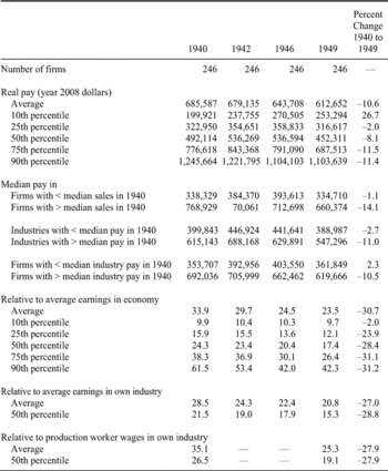
Consistent with other studies of this period, our data show a sharp decline in inequality between executives and other workers from 1940 to 1949.Footnote 13 For example, the median executive in our sample received 24 times average annual earnings in the economy in 1940, but only 17 times average annual earnings in 1949. The decline in relative compensation began during World War II, but intensified after the war. Thus, war-related forces might have been partly responsible for the compression in inequality, but other reasons are needed to explain why the compression continued after the end of the war.
We separate our analysis into two parts. First, we assess the role of government policies that might have restricted growth in executive pay relative to the rest of the workforce. War-related salary restrictions had a modest effect during World War II, but they cannot account for the slow growth in executive pay after the end of the war. We also find no evidence that the high income tax rates during this period restricted executive pay. Second, we study the role of nonregulatory determinants of the ratio of executive pay to average industry earnings, which we refer to as “relative executive pay.”Footnote 14 These determinants include individual, firm and industry characteristics that have been found to affect compensation in later decades, as well as a few other measures that might have mattered during the 1940s. We find that the decline in relative executive pay was related to a drop in the return to firm size and a growing negative correlation between compensation and industry unionization.
The economic magnitude of these effects is large, more than offsetting increases in relative pay owing to expanding firm size, rising firm profitability, and rising pay in war-related industries. Nevertheless, these factors cannot account for the continued decline in relative executive pay from 1946 to 1949. Consequently, other forces must have contributed to the contraction in relative executive pay post-1946.
DATA DESCRIPTION
Most of our analysis is based on a new data set on executive pay in the 1940s constructed from two reports published by the National Industrial Conference Board (NICB). Each report gives the remuneration (salary plus bonus) paid to each of the three highest-paid officers at two different points in time in a sample of about 500 publicly traded firms.Footnote 15 Although the names of the firms and executives are not disclosed, the reports show compensation and net sales in both years for each firm. The report published in 1948 includes remuneration and sales for 1942 and 1946, while the report published in 1951 includes similar information for 1940 and 1949.Footnote 16
The NICB data are based on proxy statements and private reports filed with the Securities and Exchange Commission (SEC), and therefore the information is arguably more accurate than survey data.Footnote 17 However, the reports do not describe the sample selection methods used by the NICB. The raw data are not likely to present a representative view of changes in the distribution of earnings over time because the 1948 report contains a significantly larger sample (762 firms) than the 1951 report (545 firms).
To compare the distribution of pay across all four years in a consistent manner, we restrict the sample in several ways. First, we drop nonmanufacturing firms because those included in the NICB reports do not appear to be representative of the nonmanufacturing sector.Footnote 18 Then, we use Moody's Manual of Investments to identify the firms included in each report and create a balanced panel of 246 firms that appear in all four years—we refer to these data as the NICB sample.Footnote 19 For these corporations, we use several editions of the Moody's manuals to collect financial information and other firm characteristics.
The final data set appears to be representative of most manufacturing corporations in the economy, since changes in the net sales of the sampled firms are similar to changes in aggregate corporate income and gross receipts per firm in the manufacturing sector. Moreover, the industrial composition of the NICB sample is similar to that of manufacturing firms that traded on the New York Stock Exchange (NYSE).Footnote 20
Since not all firms report the compensation of all three officers in every year, changes in the distribution of pay overtime could be driven by changes in the number or rank of officers. Therefore, we drop observations where we do not observe an officer of the same pay rank in the same firm in all four years.Footnote 21 The final sample covers 631 executives in each year. The evolution of compensation in the final sample appears to be representative of the salaries of top earners, as changes in NICB compensation relative to average earnings in the economy are similar to changes in the top shares of the aggregate distribution of wages and salaries from Thomas Piketty and Emmanuel Saez.Footnote 22 Thus, our findings are likely representative of the remuneration of top executives in all publicly traded manufacturing firms in the economy.
The NICB sample has limits because it does not track individuals over time and it does not report annual changes in pay. Because some aspects of our analysis hinge on studying annual changes in pay for an individual executive, we also use the annual data set on executive pay constructed by Frydman and Raven E. Saks.Footnote 23 Collected from firms’ proxy statements and other corporate reports, the Frydman-Saks sample contains annual information on the compensation of top executives in about 70 large publicly traded manufacturing firms with an average of six officers per firm in each year.Footnote 24 These firms are substantially larger than the firms in the NICB sample, so the decline in executive pay is more pronounced. Despite its many advantages, the Frydman-Saks sample is too small to study differences across industries.
Trends in Executive Pay
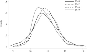
The 1940s represent a unique period of decline in the real value of top executive pay. Figure 1 shows the distribution of remuneration relative to the price level in each year of the NICB sample. The real value of pay rose at most points of the distribution from 1940 to 1942, but then decreased from 1942 to 1946 and fell further from 1946 to 1949. The combined drop in executive compensation from 1940 to 1949 was substantial; the average decreased 11 percent and the median decreased 8 percent.
DISTRIBUTION OF LN(REAL REMUNERATION)

Executive pay also fell sharply relative to the remuneration of other workers during this period. As shown in Table 1, average executive pay decreased 30 percent relative to average earnings in the economy, and it fell by a similar amount when compared to average earnings or production worker wages in the officer's own industry.Footnote 25 This compression was relatively large for most executives in the sample, as more than three-quarters of the sample experienced a decline of at least 20 percent in pay relative to average earnings. The distribution of pay across executives in the NICB sample did not narrow as much, so we focus on explaining the contraction in pay between executives and other workers, treating executives as a (relatively) homogeneous group.
SUMMARY STATISTICS ON EXECUTIVE PAY

Notes:
The sample includes 631 executives in each year. The 39 percent are the highest paid in their firm, 33 percent are the second highest paid, and 28 percent are the third highest paid. Executive pay is defined as salary plus bonus. Average earnings in the economy are average wages and salaries per full-time equivalent worker. Average earnings in own industry is wages and salaries per full-time equivalent employee. Average production worker wages in own industry is production worker wages divided by the number of production workers. Real pay is in year 2008 dollars, using the Consumer Price Index.
Sources:
Executive pay is from the National Industrial Conference Board, “Top Executive Compensation” (1948, 1951). See the text for details. Average earnings in the economy are from the National Income and Product Accounts, table 6.6 (downloaded May 2009). Average industry earnings are from the National Income Supplements to the Survey of Current Business (1951, 1958). Average production worker wages are from the Census of Manufactures (1939, 1947).
EXPLAINING THE TRENDS IN EXECUTIVE PAY: GOVERNMENT REGULATIONS
Explicit Restrictions on Earnings
As part of the command economy during World War II, the federal government instituted restrictions on salaries and wages that may have reduced top incomes relative to the rest of the earnings distribution. With the aim to restrain inflationary pressures, Roosevelt introduced two restrictions on high salaries on October 2nd, 1942: a cap on top salaries, and a broader limit on salary increases.Footnote 26 The salary cap limited labor earnings to an amount that would not exceed $25,000 after federal income taxes were paid.Footnote 27 The restriction against salary increases prohibited salaries in excess of $5,000 from rising above their level of September 15, 1942.
The salary cap was immediately controversial. It received wide support from labor unions, which perceived it as a way to ensure that wage earners did not unequally bear the burdens of the war and to limit firms from profiting from the war effort.Footnote 28 On the other hand, opponents argued that the cap would only affect a small number of individuals without keeping inflation at bay or improving the economy. Opponents also viewed the cap as an attack on enterprises and their executives, who were already subjected to “equality of sacrifice” through a progressive tax schedule. Congress repealed the cap only six months after the law was signed so, in the end, the cap had no direct impact on high incomes.
In contrast to the salary cap, the prohibition against salary changes was enforced until November 1946. However, exceptions were allowed to correct maladjustments or inequalities, to aid in the prosecution of the war, or for individual merit raises, promotions, reclassifications, and productivity increases as determined by previously established salary agreements. To change salary and bonus payments outside of these provisions, a firm could request approval from the Salary Stabilization Unit.Footnote 29 High penalties were imposed to ensure that companies did not violate these regulations.Footnote 30 From 1942 to 1946 the unit processed about 750,000 applications (equivalent to roughly 30 percent of covered individuals) for permission to increase salary or bonus payments, suggesting that firms took these regulations seriously.
Prior work has found that restrictions prohibiting wage (i.e., wages and salaries lower than $5,000 per year) increases reduced income inequality because exceptions were granted more often to low-income workers.Footnote 31 Similarly, the prohibition against salary increases may have contributed to the compression at the top of the distribution if these restrictions were more binding than the limits on wages.
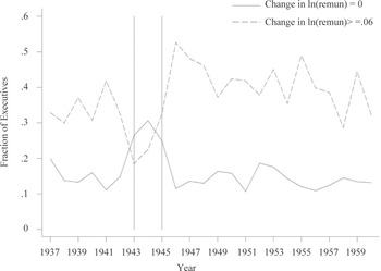
To assess the impact of the salary regulations on executive pay, we use annual data from the Frydman-Saks sample. As shown in Figure 2, about 15 percent of executives received no salary increase (defined as salary plus current bonus) in the prewar and postwar periods.Footnote 32 By contrast, 27 percent of them received no pay increase from 1943 to 1945. Therefore, the regulation may have prevented some salary changes during the war. However, its influence was not strong, as about 25 percent of the executives in this sample still obtained large wage increases, defined as larger than the average change in pay in nonwar years, when the regulation was in place (dashed line in Figure 2).
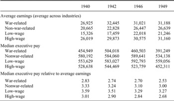
We also use industry-level data to assess the relative impact of the wage and salary restrictions on the distribution of income. The National War Labor Board (NWLB), which was in charge of regulating wages lower than $5,000 per year, was more likely to grant exceptions in low-wage industries.Footnote 33 If wage restrictions were influential, we would expect more compression between executive and workers in industries that had lower wages in the prewar period. To evaluate this hypothesis, we define low-wage industries as the following 2-digit SIC categories: lumber, textiles, tobacco, apparel, and leather products.Footnote 34 The median of average pay in these industries was $15,000 in 1940, compared with $26,000 in other industries. From 1942 to 1946 average earnings rose more and relative executive pay shrank more in low-wage industries (see Table 2). By contrast, relative executive pay increased more in low-wage industries from 1940 to 1942 and from 1946 to 1949. These patterns are consistent with war-related wage policies boosting workers’ pay (and reducing relative executive pay) in low-wage industries during the war, but the effect seems to have dissipated after the regulations were lifted.
FRACTION OF EXECUTIVES WITH ZERO OR POSITIVE CHANGE IN REMUNERATION

In addition, the NWLB was more likely to allow wage increases in war-related industries to “aid in the prosecution of the war.” The Salary Stabilization Unit may have also granted exceptions to salary restrictions for top executives in these industries, so there is no clear prediction for the net effect on executive pay relative to other workers. Empirically, salary regulations appear to have affected executives differently in war-related industries.Footnote 35 In the Frydman-Saks sample, executives in non-war-related industries were more likely to experience no change in remuneration during the war than managers in war-related industries. However, the lower incidence of salary freezes does not seem to have affected the level of executive pay. In both the Frydman-Saks and NICB samples, median executive remuneration fell more in war-related industries from 1942 to 1946 than in other industries. Nevertheless, when we compare median executive earnings to average industry earnings, we find that relative executive pay declined less in war-related than in other industries during the war period.
AVERAGE EARNINGS AND RELATIVE EXECUTIVE PAY BY INDUSTRY

Notes:
Out of a total of 27 industries, we identify six as war-related industries and eleven non-war-related industries. There are five low-wage industries and twelve high-wage industries. See the text and the Appendix for the list of industries in each category. The top panel shows the average across industries of average industry earnings (within industry), measured in year 2008 dollars. The middle panel shows the average across industries of median executive pay within each industry. The bottom panel shows the logarithm of the top panel relative to the middle panel.
Sources:
See the text and the Appendix.
In summary, wage and salary policies might have had some effect on reducing executive pay relative to the earnings of other workers from 1942 to 1946. However, this effect appears relatively modest and did not persist after the regulations were lifted.
Effect of Tax Policy
Another way in which the government might have affected the distribution of income is through tax policy. Specifically, the reduction in relative executive pay could be the result of an increase in top marginal tax rates on labor income or a reduction in tax rates on low incomes. An extensive literature in public finance has found that only high-income earners respond to changes in tax rates, so we focus on the effect of tax rates on the level of executive pay.Footnote 36 A priori, the effect of taxes on pay may have been substantial since the difference between pretax and after-tax remuneration widened dramatically during the 1940s.Footnote 37
The literature concerned with how taxable income responds to taxes usually expresses an individual's income as a function of his or her “net-of-tax rate” on labor incomeFootnote 38

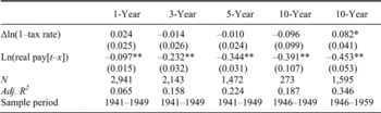
The parameter of interest is β, the “elasticity of taxable income,” defined as the percent change in pretax income when the net-of-tax rate (1–τ) increases by 1 percent, where τ is the marginal tax rate. Mostly based on data from the last thirty years, the current consensus is that β is between 0.1 to 0.4.Footnote 39 Estimates using data prior to the 1980s suggest that β was smaller or even negative in earlier decades.Footnote 40 To estimate β in the 1940s, we follow the literature and regress changes in executive pay on changes in the net-of-tax rate. The regression is specified in changes rather than levels because the progressivity of the tax system creates a mechanical correlation between the level of tax rates and the level of pay. By examining changes in tax rates, we identify the effect of taxes from reforms that alter the tax rate faced by each individual. To ensure that the net-of-tax rate is purely a function of tax policy, we calculate the tax rate in year t as the rate that would have applied to the individual if his income had remained at the same level in real terms as it was in the previous year.Footnote 41
CORRELATION OF CHANGES IN TAX RATES AND CHANGES IN REAL EXECUTIVE PAY

∗ = Significant at the 5 percent level.
∗∗ = Significant at the 1 percent level.
Notes:
The figures in parentheses are standard errors, which are clustered by year in columns 1 to 3 and by individual in columns 4 and 5. Each regression also controls for log of the firm's market value, the rate of return, job title dummies for chairman, president, executive vice president, and vice president, an indicator for director of the board, an indicator for whether the executive changed jobs during the year, and a dummy to capture changes in director status.
Sources:
Proxy statements and 10-Ks of 77 large firms. See Frydman and Saks, “Executive Compensation.”
We cannot follow specific individuals over time in the NICB data, so we use the Frydman-Saks sample for this analysis.Footnote 42 Among the covariates, we include the logarithm of lagged real remuneration to account for mean-reversion in income, which may cause higher-income executives to experience larger reductions in pay.Footnote 43 We calculate an executive's marginal income tax rate assuming that his income is equal to the remuneration paid by his firm and that he files jointly with a spouse.
As shown by the first column of Table 3, changes in remuneration were unrelated to changes in tax rates. The coefficient β is precisely estimated and we can reject the hypothesis that the elasticity is greater than 0.1 with a p-value smaller than 0.01. One possible reason for a small estimate of β is that compensation may adjust slowly to changes in tax policy. To assess the delayed response to taxes, the remaining columns of Table 3 report the regressions results for 3-year changes, 5-year changes, and 10-year changes in pay and net-of-tax rates. The sample size of the 10-year change regression is fairly small because we observe few individuals for such a long period. To increase the sample size, we extend the sample to include changes in remuneration through the 1949–1959 period. In every case, we can reject the hypothesis that the elasticity was greater than 0.2, and in all specifications except one, we can reject an elasticity greater than 0.1.Footnote 44
In sum, we do not find a strong positive relationship between changes in pay and changes in the net-of-tax rate. The lack of response of compensation to the rise in tax rates means that after-tax pay fell by even more than pretax pay during this period. Average real after-tax compensation dropped 24 percent from 1940 to 1949, more than double the 11 percent decrease in average real pretax pay. Thus, the disposable incomes of corporate executives contracted considerably during this period.
EXPLAINING THE TRENDS: NONREGULATORY DETERMINANTS
A large literature in corporate finance has found various individual, firm, and industry characteristics to be important determinants of executive pay in recent decades.Footnote 45 Studies of income inequality also relate disparities in top incomes to other factors, such as the power of unions and the returns to skills.Footnote 46 Following these two literatures, we study the role of nonregulatory determinants of relative executive pay.
Determinants of the Level of Executive Pay and Earnings Inequality
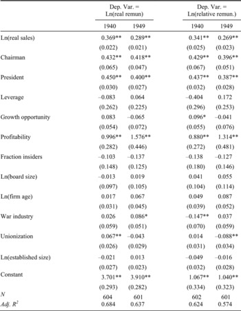
The determinants of the log level of real executive compensation in 1940 and 1949 are estimated using OLS regressions reported in columns 1 and 2 of Table 4.Footnote 47 See the Appendix for definitions and sources of all variables. Consistent with prior findings in the literature, we find positive returns to being the president or chairman of the corporation.Footnote 48 This return did not change appreciably from 1940 to 1949, making it an unlikely candidate to explain the drop in relative executive pay.
DETERMINANTS OF EXECUTIVE PAY IN 1940 AND 1949

∗ = Significant at the 10 percent level.
∗∗ = Significant at the 5 percent level.
Notes:
Numbers in parentheses are standard errors clustered by firm. Real remuneration is the value of salaries and bonus in year 2008 dollars. Relative remuneration is the ratio of nominal remuneration to average industry production worker wages. For the definition of all other variables, see the Appendix.
Sources:
National Industrial Conference Board, “Top Executive Compensation” (1948, 1951). See the text for details.
Turning to firm characteristics, pay was higher in larger firms. We measure firm size as the logarithm of the real value of net sales, but these results are robust to using the firm's market value or total assets instead. This positive correlation is consistent with prior studies, which find firm size to be one of the main correlates with executive pay.Footnote 49 The returns to firm size fell noticeably during the sample period, as the coefficient on sales was 20 percent lower in 1949 than in 1940.
Executive pay was also higher in more profitable firms, as measured by return on assets. Other observable firm characteristics, including capital structure (proxied by the book leverage ratio), the firm's growth opportunities (measured by the market-to-book ratio), the firm's age (measured by the year of incorporation), the size of the board of directors, and the fraction of insiders (current managers of the firm) on the board, had little impact on the level of pay.Footnote 50
When considering industry characteristics, executive pay was slightly higher in more unionized industries in 1940, but the correlation had become negative by 1949.Footnote 51 The decline in relative executive pay in highly unionized industries relative to other industries may have been due to the growing power of unions over the 1940s.Footnote 52 In the 1930s large corporations were mostly able to defend against unions even though unions’ organization and membership was strengthening with the passage of the National Labor Relations Act.Footnote 53 Union membership expanded markedly during World War II from 26 percent of nonagricultural employment in 1940 to 34 percent in 1945 and remained high for the rest of the decade.Footnote 54 Two plausible factors contributing to this expansion were a reduction in employer opposition due to the wartime economic growth, and government actions aimed at minimizing labor disputes to facilitate the war effort.Footnote 55 Strike activity was also elevated, likely causing managers to take unions’ concerns seriously. The growing negative correlation between unionization and executive pay during the 1940s suggests that executives were limited to reaping a smaller share of profits as the bargaining power shifted towards organized labor.Footnote 56
Executives in war-related industries were remunerated more handsomely in 1949, even though compensation was similar in war-related and nonwar-related industries in 1940. This widening pay gap might have reflected a rise in the demand for war-related products, or it may also have been the result of laxer enforcement of wartime regulations on salaries in these industries. Finally, we allow compensation to be affected by the size of the typical firm in their industry. If firms compete for scarce managerial talent, the overall growth of firms in an industry may lead to an increase in executive pay in that industry, even after conditioning on the size of the executive's firm.Footnote 57 However, we do not find any correlation between executive pay and the number of production workers per establishment in the industry.
To understand the changes in inequality between executives and workers, we would like to study whether these nonregulatory factors were also important determinants of the gap between executive compensation and the wages of the workers in the executive's firm. Such a specification would allow us to net out many unobservable factors that are correlated with firm and industry characteristics. We lack information on workers’ wages at the firm level, so we use workers’ wages at the industry level—in this case, the average wage of production workers in the 2-digit SIC industry. Columns 3 and 4 of Table 4 present the determinants of the logarithm of relative executive pay in 1940 and 1949. Overall, the results for relative pay are similar to the results for the real level of executive compensation. In particular, the positive return to firm size diminishes between 1940 and 1949, while the negative correlation between pay and unionization strengthens over this period. Also, relative executive pay rose more in war-related industries.
Since the results are largely similar for the level of executive pay and its ratio to workers’ earnings, for the remainder of the article, we focus on results using relative executive pay as the dependent variable. However, it is useful to keep in mind that most of the variation in relative executive pay is driven by executive compensation (the numerator) rather than average industry pay (the denominator).
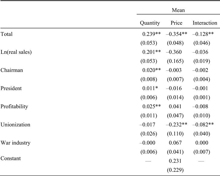
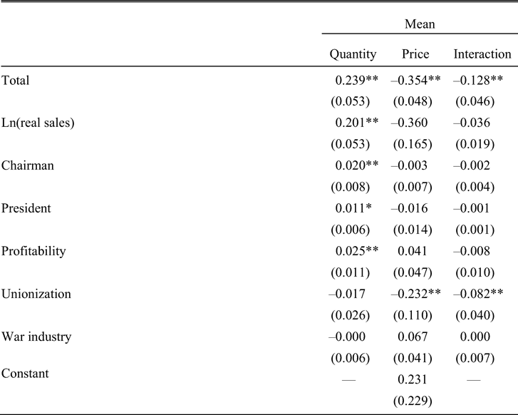
OAXACA DECOMPOSITION OF CHANGES IN AVERAGE RELATIVE EXECUTIVE PAY, 1940–1949
∗ = Significant at the 10 percent level.
∗∗ = Significant at the 5 percent level.
Notes:
Numbers in parentheses are standard errors and are clustered by firm. Relative remuneration is the ratio of nominal remuneration to average industry production worker wages. See the Appendix for definitions of the covariates.
Sources:
National Industrial Conference Board, “Top Executive Compensation” (1948, 1951). See the text for details.
Decomposing Changes in Executive Pay
To understand how each variable has affected relative executive pay over time, the left-hand panel of Table 5 presents an Oaxaca decomposition based on the OLS regression results. This analysis divides the change in average relative compensation from 1940 to 1949 into a portion attributable to the change in the quantity of each independent variable, a portion attributable to the change in the price (i.e., estimated coefficient) of each independent variable, and a portion attributable to the interaction between quantities and prices. Specifically, we calculate

where  is the average of the dependent variable,
 is the average of the independent variables, and β is the vector of estimated coefficients. An extensive literature has used Oaxaca decompositions to analyze the determinants of changes in earnings distributions.Footnote 58 For simplicity, we present decompositions based on regressions that exclude variables without a meaningful correlation with executive pay, but results are similar when all variables are included.
The decompositions reveal two main factors that constrained executive pay relative to average industry pay during this period: the decline in the return to firm size, and the emergence of a negative correlation between unionization and remuneration.Footnote 59 The economic magnitudes of these effects are substantial and statistically significant. Had the returns to size and unionization remained at their 1940 values, average relative executive pay would have been 0.59 log points higher in 1949 than was observed (0.36 due to unionization and 0.23 due to firm size). Given that average relative pay fell by 0.26 log points during this period, these two factors more than account for the decline in executive pay relative to other workers. Offsetting these factors were increases in average firm size and average firm profitability. The relative increase in pay in war-related industries also boosted relative executive compensation by 0.07 log points, although this effect is imprecisely estimated.
The Oaxaca decompositions reveal the influence of quantities and prices on changes in average compensation over time. Because the distribution of executive pay is usually highly skewed, the mean may give a biased view of the changes for the typical executive. Focusing on the average in the 1940s may not be too problematic because changes in the mean and median during this period were fairly similar (see Table 1).Footnote 60
Persistence and Timing of the Reduction in Relative Executive Pay
To gain insight into whether the factors that reduced relative executive pay from 1940 to 1949 had a long-lasting impact on the distribution of income, we expand our analysis into the 1950s. To this end, we use the last NICB report to disclose information at the firm level, which details the salaries and bonuses awarded to the three-highest paid executives in 560 manufacturing firms in 1955. Using the firm's net sales and industry description, we match 126 firms from this sample to the firms in the 1940–1949 balanced panel.Footnote 61 Similar to the previous results, an Oaxaca decomposition reveals that average relative executive pay was also reduced from 1940 to 1955 by declines in the coefficients on firm size and unionization, while increases in average firm size boosted pay. The lack of recovery for so long after the end of World War II indicates that the war is unlikely to be the sole explanation for the drop in relative pay and suggests that these factors may help explain why top incomes did not keep up with the rest of the economy for the next thirty years.Footnote 62
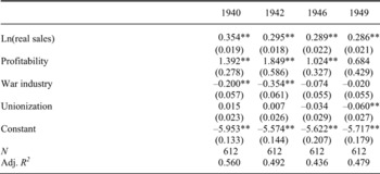
An advantage of our data is that we can analyze changes in pay within the 1940s decade. We explore the timing of the reduction in the returns to firm size and unionization by estimating OLS regressions for executive pay relative to average industry earnings in each of the four years of the NICB panel (see Table 6).Footnote 63 The higher-frequency data reveal that the drop in the return to firm size occurred mostly between 1940 and 1942, and it remained low throughout the rest of the decade. Thus, the change in the relation between relative pay and firm size was rather sudden and persistent. When using these coefficients in an Oaxaca decomposition (not shown), the drag on relative pay due to the change in the return to firm size was much larger than the actual decrease in relative pay from 1940 to 1942, as this negative effect was partly offset by other factors. The coefficient on unionization became gradually more negative throughout the decade, suggesting that the power of labor unions strengthened steadily over time. Not surprisingly, the narrowing of the pay gap between war-related and other industries occurred mainly between 1942 and 1946.
DETERMINANTS OF RELATIVE EXECUTIVE PAY OVER TIME

∗ = Significant at the 10 percent level.
∗∗ = Significant at the 5 percent level.
Notes:
Numbers in parentheses are standard errors and are clustered by firm. Relative executive pay is the ratio of nominal remuneration to average industry earnings. See the Appendix for definitions of the covariates.
Sources:
National Industrial Conference Board, “Top Executive Compensation” (1948, 1951). See the text for details.
INTERPRETATION AND CONCLUSION
Mirroring the decline in the aggregate share of wages and salaries of top earners, executive pay rose much less than the average earnings of the workforce from 1940 to 1949. Top officer compensation also failed to keep up with average production worker earnings in their own industry. Declines in relative executive pay were pervasive, as relative pay fell for almost all top corporate officers of publicly traded manufacturing firms.
No single cause was responsible for the large contraction in relative executive pay during this period. Government regulation in the form of taxation and restrictions on salaries and wages may have played a modest role in the first half of the 1940s, but their direct effects seem to have been small and they cannot account for the persistently low level of relative pay after the end of the war. We find larger and more prolonged roles of several firm and industry characteristics. First, relative executive pay fell more in highly unionized industries than in other industries, suggesting that the power of labor unions to restrict officers’ remuneration strengthened gradually over the decade. Second, the return to firm size declined from 1940 to 1942 and remained relatively low until 1949. These regulatory and nonregulatory forces were appreciable, but they cannot fully explain the changes in the income distribution during the 1940s. Thus, other factors must have also contributed to the decline in relative executive pay during this period.
Appendix
FIRM-LEVEL DATA
Net sales: Net sales as reported by Moody's. This measure differs by more than 5 percent from the NICB's reported net sales in only 4 percent of firms. The NICB occasionally reports total sales instead of net sales, so it is less consistent than the Moody's measure.
Total assets: Total assets as reported by Moody's.
Market value of equity: Total number of common shares outstanding multiplied by the average of the year's low and high share price as reported by Moody's. For the 165 firms for which we have the end-of-year share price and shares outstanding from CRSP, the correlation between CRSP market value and Moody's market value is 0.98.
Book leverage ratio: Debt in current and long-term liabilities divided by total assets as reported by Moody's.
Growth opportunities: The sum of market value of equity, current liabilities and long-term liabilities divided by total assets as reported by Moody's.
Firm profitability (return on assets): Net income divided by total assets in the previous year as reported by Moody's.
Firm age: Current year minus the year of incorporation as reported by Moody's.
Board size: Total number of members of the board of directors as reported by Moody's.
Fraction of insiders: Fraction of the board of directors who were also executives of the firm during the year as reported by Moody's.
INDUSTRY-LEVEL DATA
Average production worker wage: Total production worker wages divided by the number of production workers as reported by the 1939 and 1947 Census of Manufactures. We use the most disaggregated industry definition possible, which leads to 37 different values across 15 different 2-digit industry categories. We assign the 1939 data to 1940 NICB data and the 1947 data to 1949 NICB data.
Number of production workers per establishment: Total number of production workers divided by total number of establishments as reported by the 1939 and 1947 Census of Manufactures. See further details under “Average production worker wage.”
Industry productivity: Total value added divided by the number of production workers as reported by the 1939 and 1947 Census of Manufactures. See further details under “Average production worker wage.”
Average industry earnings: Total wages and salaries divided by the number of full-time equivalent employees as reported by the 1951 and 1958 editions of the National Income Supplement to the Survey of Current Business. Annual data are reported for 2-digit SIC industries.
Unionization: For 1940 to 1949 we use the fraction of wage earners under written union agreements as reported in various Bureau of Labor Statistics (BLS) Bulletins. The BLS reports data for 52 manufacturing industries, which they divide into groups with fraction unionized between 1–20 percent, 20–40 percent, 40–60 percent, 60–80 percent, and 80–100 percent.Footnote 64 The BLS does not associate industry codes with each industry name, so we assign a code to each industry name based on 1945 SIC codes. Then we calculate the average proportion unionized for each 2-digit industry using employment shares from the 1940 Census as weights. These reports provide data for 1938, 1941, 1944, 1945, and 1946. We assign the 1938 unionization data to the 1940 NICB data, the 1941 unionization data to the 1942 NICB data, and the 1946 unionization data to the 1946 and 1949 NICB data. To estimate unionization in 1955, we extrapolate the 1949 fraction unionized using the growth rate in union density from 1947 to 1953 reported in Bain and Price, Profiles. These density estimates are reported for eight industry categories, which are a combination of one or several 2-digit SIC industries.
War-related industries: Firms in the following 2-digit categories: chemicals, rubber products, fabricated metal products, electrical machinery, other machinery, and transportation equipment.
Corporate income of the manufacturing sector: Total corporate income before federal and state income and excess profits taxes as reported by the 1951 edition of the National Income Supplement to the Survey of Current Business.
Receipts per firm in the manufacturing sector: Gross sales of firms reporting positive net income divided by the number of tax returns with positive net income as reported by the Statistics of Income.
Industry classification: The industry names used in the NICB reports correspond to various levels of aggregation (two examples are “breweries” and “general industrial machinery”) and are not linked to any industry codes. Therefore, we match the reported industry names to Standard Industrial Classification (SIC) codes from 1945. The firms fall into 22 different 2-digit industrial categories, with the majority (87 percent) in manufacturing industries. The industrial composition of the manufacturing firms in the NICB data is fairly similar to that of firms traded on the NYSE.Footnote 65 By contrast, the nonmanufacturing firms in the NICB data do not appear to be representative of the nonmanufacturing economy more broadly.