





1. Introduction
At radio frequencies, magnetically active M dwarfs are capable of emission with intensity far exceeding that from the Sun. In addition to slowly-varying quiescent emission ascribed to gyrosynchrotron radiation (e.g. Kundu & Shevgaonkar Reference Kundu and Shevgaonkar1985; Pallavicini et al. Reference Parker1985; Williams et al. Reference Yiu, Vedantham, Callingham and Günther2014), many M dwarfs produce transient bursts caused by a coherent mechanism: electron cyclotron maser (ECM) emission (e.g. Gary et al. Reference Gordon1982; Kundu et al. Reference Lacy1987; Villadsen & Hallinan Reference Wang2019) or plasma emission (e.g. Stepanov et al. Reference Thejappa, MacDowall and Bergamo2001; Osten & Bastian Reference Osten and Bastian2006; Callingham et al. Reference Callingham2025).
A central question in the study of this emission regards the transition along the main sequence from solar-like bursts, primarily originating from plasma emission, to the rotationally modulated ECM emission exhibited by ultracool dwarfs (e.g. Hallinan et al. Reference Hallinan2007; Lynch et al. Reference Lynch, Mutel and Güdel2015; Hallinan et al. Reference Harvey-Smith2015; Rose et al. Reference Samus’, Kazarovets, Durlevich, Kireeva and Pastukhova2023). Both have been observed from M dwarfs (e.g. Villadsen & Hallinan Reference Wang2019; Zic et al. Reference Zic2019, Reference Zic2020; Callingham et al. Reference Callingham2025). Detailed monitoring of individual M dwarfs is instrumental for identifying each type and can be used to probe the plasmas and magnetic fields from which the emission originates (e.g. Villadsen & Hallinan Reference Wang2019; Bloot et al. Reference Bloot2024; Callingham et al. Reference Callingham2025). This is of particular interest for dwarfs of spectral type
 $\sim$
M4 (e.g. Morin et al. Reference Murphy2008), with masses near the
 ${\sim} 0.35\,{\rm M}_\odot$
transition in interior structure below which stars are fully convective (Chabrier & Baraffe Reference Chabrier and Baraffe1997).
Positions of all 154 GCNS stars with median distance estimates (Gaia Collaboration 2021b) below 85 pc, shown as blue stars, selected within the bounds marked by the dark blue rectangle for the search described in Section 2.1. WW PsA and its binary companion TX PsA are marked by the green circle. Background: Stokes
 $I$
image showing Footprint A of DINGO Tile 0 (see Rhee et al. Reference Ricker2023) from the ASKAP scheduling block SB65210. The positions of the stars are proper motion corrected to the epoch J2024.7, corresponding to this observation.

Coherent, rotationally modulated emission from M dwarfs can be auroral in nature (Hallinan et al. Reference Harvey-Smith2015; Zic et al. Reference Zic2019), corresponding to a dipolar magnetic field (see the model presented by Leto et al. Reference Leto2016), but in some cases is better modelled with more complicated magnetic field configurations (Lynch et al. Reference Lynch, Mutel and Güdel2015). Further complicating the matter, the stochastic bursts from the M1Ve dwarf AU Mic were recently found to have variations in fractional polarisation matching the rotation period, explained by auroral ECM emission (Bloot et al. Reference Bloot2024).
In recent years, the Australian SKA Pathfinder (ASKAP; Hotan et al. Reference Ibañez Bustos, Buccino, Flores, Martinez and Mauas2021) has enabled the discovery of many radio stars (e.g. Pritchard et al. Reference Pritchard, Murphy, Heald, Wheatland, Kaplan, Lenc, O’Brien and Wang2021, Reference Ravi2024; Rose et al. Reference Samus’, Kazarovets, Durlevich, Kireeva and Pastukhova2023; Driessen et al. Reference Dulk2024; Das et al. Reference Driessen2025). Many of the ASKAP surveys used in these radio star searches have integration times of 12–15 min (e.g. McConnell et al. Reference Melrose and Dulk2020; Murphy et al. Reference Mutel, Peterson, Jaeger and Scudder2021), allowing rapid coverage of wide areas of the sky. However, for detailed investigations of individual stars, such surveys are limited in the amount of observation time they contribute.
In contrast, the ASKAP Deep Investigation of Neutral Gas Origins survey (DINGO; Rhee et al. Reference Ricker2023) targets two adjacent
 $\sim$
30 deg
 $^2$
tiles of extragalactic sky, with a planned 1 600 h of observation time on each tile, split between two frequency ranges:
 $\text{Low-}z$
targeting the 1 420 MHz H i line at redshifts
 $0 \lt z \lt 0.1$
, and
 $\text{High-}z$
targeting
 $0.25 \lt z \lt 0.4$
. This presents an opportunity for long-duration radio monitoring of any radio stars present in the DINGO survey area.
In this paper we present a detailed investigation of the radio emission from the M4V dwarf WW PsA including coherent bursts detected in a search for radio emission from stars within 85 pc with DINGO. In Section 2 we detail our observations and data analysis, including our search method as well as our analysis of the bursts and quiescent emission from WW PsA. In Section 3 we discuss the significance of our search for the population statistics of nearby radio stars, describe the known properties of WW PsA, and interpret the observed emission. In particular, we investigate the possibility that the bursts are due to rotationally modulated ECM emission.
2. Observations and data analysis
2.1. Search method and detection of WW PsA
To construct a sample of stars for our search, we selected all objects in the Gaia Catalogue of Nearby Stars (GCNS; Gaia Collaboration 2021b) within a distance of 85 pc in the
 $33.45\,\mathrm{deg}^{2}$
region defined by the bounds
 $22^{\mathrm h} 32^{\mathrm m} 40^{\mathrm s} \lt \alpha \lt 22^{\mathrm h} 59^{\mathrm m} 30^{\mathrm s}$
and
 $-35^\circ 13^\prime \lt \delta \lt -29^\circ 19^\prime$
. This region corresponds to Footprint A of DINGO Tile 0 (see Rhee et al. Reference Ricker2023), as shown in Figure 1. We used the J2016.0 coordinates and median distance estimates dist_50 provided in the GCNS (Gaia Collaboration 2021a, b) to select the sample. This resulted in 154 stars, the positions of which are also shown in Figure 1.
For each star, we used DStools
Footnote
a
(Pritchard Reference Pritchard2025) to produce a dynamic spectrum and lightcurve in Stokes
 $I$
,
 $Q$
,
 $U$
, and
 $V$
Footnote
b
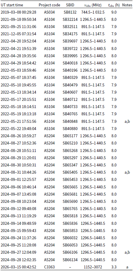
at the proper motion corrected coordinates in each of the 18 DINGO full-survey observations (project code AS204) listed in Table 1. Although our sample of stars was selected based on Footprint A of DINGO Tile 0, some of these observations were conducted using Footprint B. The offset between the footprints was small enough to allow dynamic spectrum creation for all stars in our sample in each epoch. This amounted to 144 h of data per object.
Summary of radio observations searched for polarised emission from WW PsA by producing dynamic spectra and lightcurves. Observations under the project code AS204 were included in the search for emission from nearby stars described in Section 2.1.

Table 1. Long description
35 ASKAP observations from March 2019 to September 2024 and an ATCA observation from March 2026 are summarised. The columns are the UT start time, project code (AS034, AS104, AS204, or C3363), ASKAP Scheduling Block ID (where applicable), observing frequency (744.5–1032.5 MHz for the single AS034 observation, 891.5–1147.5 or 1296.5–1440.5 MHz for the AS104 and AS204 observations, and 1152–3072 MHz for the C3363 observation), observation duration (9.0 h for the AS034 observation, 7.9 or 8.0 h for the AS104 and AS204 observations, and 3.3 h for the C3363 observation), and notes. Note (a) says "Stokes I dynamic spectrum and lightcurve produced and inspected" for SB40848, SB65405, SB66106, and the ATCA observation. Note (b) says "Circularly polarised burst detected" for SB40848, SB65405, and SB66106.
(a) Stokes I dynamic spectrum and lightcurve produced and inspected.
(b) Circularly polarised burst detected.
We produced the dynamic spectra and lightcurves using both the original 10 s time resolution and a time resolution of 5 min, in both cases using the original 1 MHz frequency resolution of the data. We flagged some bands with persistent radio frequency interference (RFI) using DStools (from the bottom of the observed frequency range to 1 315 MHz and the band 1 379–1 382 MHz), in addition to the flagging present in the visibility data as obtained from the CSIRO ASKAP Science Data ArchiveFootnote
c
(CASDA). We performed a visual inspection of the Stokes
 $V$
dynamic spectra and lightcurves, not including the other Stokes parameters as they contained artefacts caused by sidelobes from bright neighbouring sources (especially in Stokes
 $I$
). We did not find any emission above a
 $5\sigma$
detection threshold except for two bursts from WW PsA (see Section 3.2 for a description of this star).
We used DStools to perform field modelling and subtraction for the two epochs (scheduling blocks SB65405 and SB66106) in which we found bursts from WW PsA. This greatly reduced the impact of sidelobes from bright nearby sources, allowing us to make use of the Stokes
 $I$
,
 $Q$
, and
 $U$
data for these bursts. We did not perform this step in the original search as it is computationally intensive. The resulting dynamic spectra and lightcurves in Stokes
 $I$
and
 $V$
are shown in Figure 2. The burst in SB65405 had a longer duration than that in SB66106, at
 ${\sim} \mathrm{1.5}$
and
 ${\sim} \mathrm{0.5\, h}$
, respectively. The latter was much more strongly confined in frequency, being brightest in the range 1 350–1 410 MHz, with the former showing little variation in flux density across the observed band. Both had (signed) fractional circular polarisation
 $S_V/S_I \approx 1$
, however this decreased to
 $S_V/S_I \approx 0$
towards the end of the burst in SB65405. We did not detect linear polarisation in either case.
2.2. Additional archival observations of WW PsA
We searched for circularly polarised emission from WW PsA in one observation from the ASKAP Early Science Broadband Survey (Harvey-Smith et al. Reference Henry2018; O’Brien et al. Reference Osten and Bastian2019) and 16 from the DINGO pilot survey (project codes AS034 and AS104, respectively, in Table 1), totalling 137 h. Again, we performed this search by visual inspection of the dynamic spectra and lightcurves in Stokes
 $V$
. We detected one additional event: a burst in SB40848 lasting
 ${\sim} 2\,\mathrm{h}\; 35\,\mathrm{min}$
with a reversal in the sense of its circular polarisation halfway through, from right-handed to left-handed. Prior to this polarity reversal, this burst reached a maximum Stokes
 $V$
flux density
 $S_V = 5.9 \pm 0.2$
mJy, significantly brighter than those in SB65405 and SB66106. After the reversal, the burst was much fainter, reaching
 $S_V = -1.6 \pm 0.2$
mJy, comparable in magnitude to the bursts in Figure 2. We did not detect linear polarisation.
Top & Middle: Stokes
 $I$
and
 $V$
dynamic spectra of WW PsA in scheduling blocks SB65405 (left) and SB66106 (right) after field modelling and subtraction, with a time resolution of 5 min. Visibilities from baselines shorter than 500 m have been excluded. Bottom: Stokes
 $I$
and
 $V$
lightcurves for the same observations.

Top & Middle: Stokes
 $I$
and
 $V$
dynamic spectra of WW PsA in scheduling block SB40848 after field modelling and subtraction, with a time resolution of 2.5 min. Visibilities from baselines shorter than 500 m have been excluded. Bottom: Stokes
 $I$
,
 $Q$
,
 $U$
, and
 $V$
lightcurves for the same observation with a time resolution of 5 min.

The Stokes
 $I$
and
 $V$
dynamic spectra and lightcurves from SB40848, after field modelling and subtraction (and excluding visibilities from the baselines shorter than 500 m), are shown in Figure 3. The Stokes
 $I$
lightcurve reveals quiescent emission before and after the burst. We discuss the emission seen in this observation further in Section 3.3.
This search, as well as the search described in Section 2.1, only included observations from 2024 and earlier. However, we subsequently detected a burst from the later DINGO observation SB76830 using the VASTER pipeline (Wang et al. Reference West2026). This observation covered the band 1 296.5–1 440.5 MHz. The burst began at 2025–09–13
 $\sim$
16:30 UTC and continued until the end of the observation at
 $\sim$
21:15 UTC, making it
 ${\gtrsim} \mathrm{4\,h}\,{45}\,\mathrm{min}$
in duration. Its peak Stokes
 $I$
flux density in the image plane, obtained from VASTER, reached a maximum of
 $3.4 \pm \mathrm{0.2\, mJy\, beam}^{-1}$
at
 $\sim$
19:15 UTC. We leave a detailed analysis of this burst for future work, but discuss the implications of its time of arrival in Section 3.5.2.
2.3. Follow-up observation
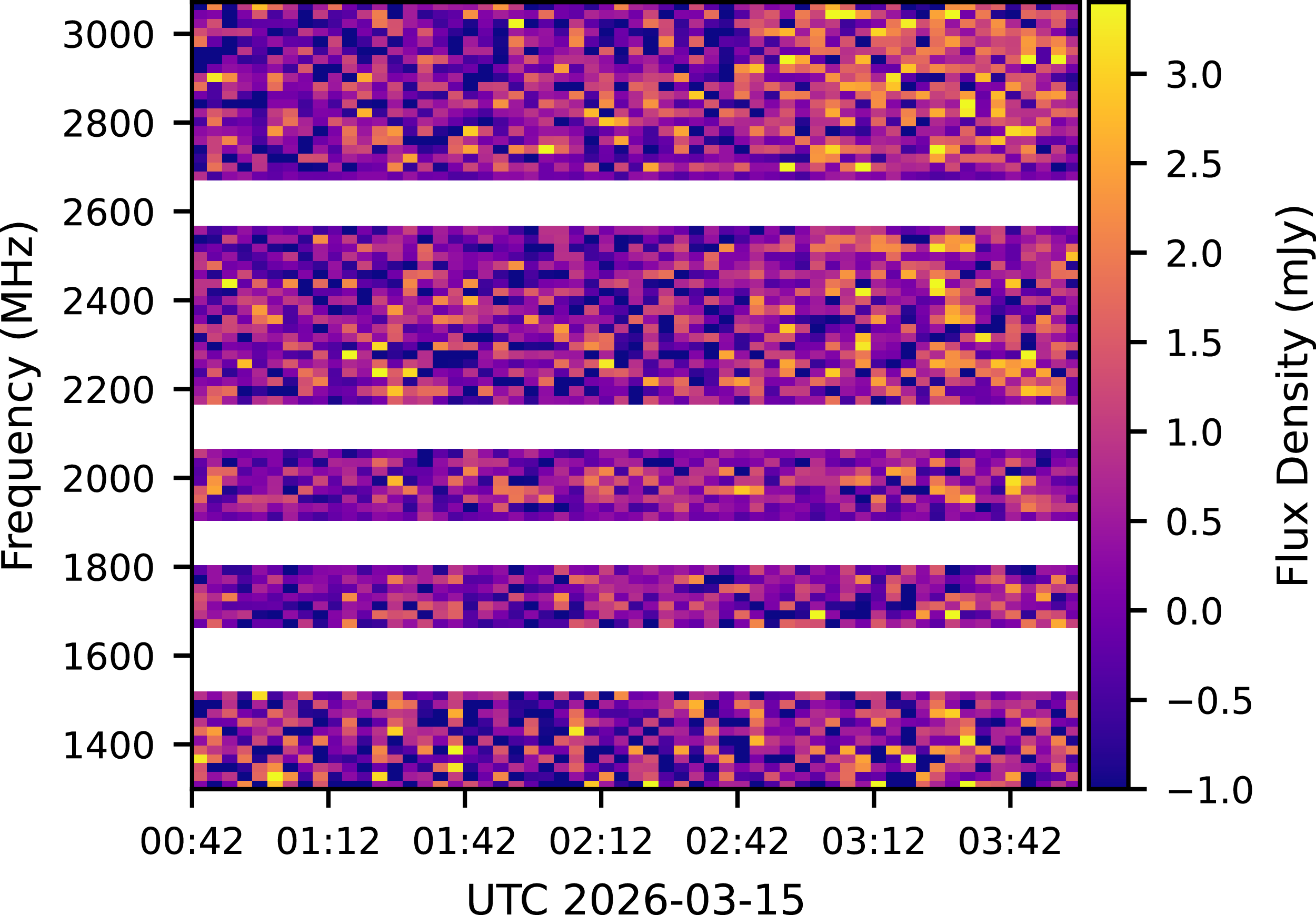
We conducted a 3.5-h radio follow-up observation of WW PsA with the Australia Telescope Compact Array (ATCA) on 2026-03-15 (project code C3363). This observation was performed in the 6C configuration using the 16 cm (L-band) receiver with a 1 920 MHz band centred on 2 112 MHz. We used PKS B1934
 $-$
638 (PKS J1939
 $-$
6342) to calibrate the bandpass response, flux scale, and polarisation leakage. We performed phase calibration with interleaved scans of PKS B2245
 $-$
328 (PKS J2248
 $-$
3235), each lasting 90 s. We flagged and calibrated the data using standard continuum data processing routines in miriad
Footnote
d
(Sault et al. Reference Sharma and Vlahos1995) and produced Stokes
 $I$
and
 $V$
dynamic spectra. We detected quiescent emission in Stokes
 $I$
, as shown in Figure 4, but we did not make a detection in Stokes
 $V$
. The quiescent emission was brighter at higher frequencies and increased in flux density towards the end of the observation.
Stokes
 $I$
dynamic spectrum from our follow-up observation of WW PsA with the ATCA. The flux density of the quiescent emission is greater at higher frequencies and increases towards the end of the observation.

2.4. Stokes I image-plane detections
Figure 5 shows a lightcurve of detections and non-detections of WW PsA, made in the Stokes
 $I$
image plane with surveys from ASKAP and the Karl G. Jansky Very Large Array (VLA; Perley et al. Reference Pritchard2011). The observations included have a variety of frequency ranges (within 0.8–4 GHz) and durations (2 min–9 h). To obtain the ASKAP detections, we cross-matched the proper motion corrected position of WW PsA to the source component catalogue, produced with the source finder package selavy (Whiting & Humphreys Reference Williams, Cook and Berger2012), which are publicly available in CASDA. Out of 104 ASKAP epochs in which WW PsA was observed, our cross-match yielded 43 detections and 61 non-detections. For the detections, Figure 5 shows the peak flux density, with the uncertainty due to the selavy fit added in quadrature with the local root mean square (RMS) noise value, also provided by selavy. For the non-detections we adopted
 $5\sigma _{\text{rms}}$
upper limits, where
 $\sigma _{\text{rms}}$
is the RMS value of the noiseMap provided by CASDA. To do this, we downloaded
 $4^\prime \times 4^\prime$
noiseMap cutouts centred on the position of WW PsA. The RMS of the cutout was therefore the noise local to WW PsA. For 27 of these non-detections, we were unable to determine
 $\sigma _{\text{rms}}$
as the noiseMap was not available on CASDA. We excluded a further 12 non-detections with
 $5\sigma _{\text{rms}} \gt 2.9\,\mathrm{mJy\,beam}^{-1}$
, as in these observations WW PsA was near the edge of the field, where the image was dominated by artefacts. The remaining 22 ASKAP non-detections are shown in Figure 5.
We performed a similar cross-match to search for detections in the 2–4 GHz VLA Sky Survey (VLASS; Lacy et al. Reference Lacy2020) Quick Look (Gordon et al. Reference Hallinan2021) catalogues. WW PsA was detected in VLASS Epoch 1 with peak flux density
 $3.60\pm 0.13\,\mathrm{mJy\,beam}^{-1}$
, scaled by a factor of 1.1 as recommended by Lacy et al. (Reference Leto, Trigilio, Buemi, Umana, Ingallinera and Cerrigone2022). This detection is reported by Yiu et al. (Reference Zarka2024). We did not obtain a detection in VLASS Epoch 2, with a
 $5\sigma _{\text{rms}}$
upper bound of
 ${\sim} 0.7\,\mathrm{mJy\,beam}^{-1}$
.Footnote
e
Lightcurve showing Stokes
 $I$
image-plane detections (coloured) and non-detections (grey) of WW PsA with ASKAP and the VLA. Uncertainties for the detections were derived by adding the Gaussian fit uncertainty in quadrature with local image RMS noise
 $\sigma _{\text{rms}}$
. Non-detections are marked as
 $5\sigma _{\text{rms}}$
upper limits, with downward arrows of length
 $\sigma _{\text{rms}}$
. As discussed in Section 2.4, only 22 of the 61 non-detections we found from ASKAP observations are shown. The ASKAP observations are labelled by project code: the ASKAP Early Science Broadband Survey (AS034), DINGO (AS104 and AS204), the Rapid ASKAP Continuum Survey (AS110; McConnell et al. Reference Melrose and Dulk2020), the survey and monitoring of ASKAP’s RFI environment and Trends project (AS115; Lourenço et al. Reference Lu2024), and the variables and slow transients survey (AS032 and AS207; Murphy et al. Reference Mutel, Peterson, Jaeger and Scudder2021).

3. Discussion and interpretation
3.1. Significance of volume-limited search
In the volume-limited search described in Section 2.1, we covered
 $2.2\times 10^{-4}$
star-hours = 2.5 star-years worth of dynamic spectra and lightcurves. Overall, this was much smaller than the recent 100 star-year search for stellar Type II radio bursts in Stokes
 $V$
dynamic spectra by Konijn et al. (Reference Kundu, Jackson, White and Melozzi2025). However, for each star their search covered only
 $\sim \!8\,\mathrm{h}$
of observation time, compared to 144 h in ours. Our search did not account for burst drift rates.
In our search we made two detections of one star out of our sample of 154 stars. From this, we obtain estimates of the on-sky surface density
 $n$
and volume density
 $\rho$
of detected radio stars within 85 pc:
 $\log _{10}(n/\text{deg}^{-2}) = -{1.5^{+0.7}_{-1.6}}$
and
 $\log _{10}\left (\rho /\text{pc}^{-3}\right ) = -{3.3^{+0.7}_{-1.6}}$
, with uncertainties given by 95% Poisson confidence intervals. Based on H
 $\alpha$
emission, the local density of magnetically active M dwarfs within 10 pc has been estimated to be
 $\sim \!0.016\,\mathrm{pc^{-3}}$
(Villadsen & Hallinan Reference Wang2019; West et al. Reference White, Jackson and Kundu2011; Henry et al. Reference Hotan2018), implying we detected at most
 $\sim$
20% of magnetically active M dwarfs in our sample volume. However, restricting the sample radius to 25 pc, which still includes the only detected star, gives a density
 $\log _{10}\left (\rho /\text{pc}^{-3}\right ) = -{1.7^{+0.7}_{-1.6}}$
, consistent with up to a 100% detection rate for magnetically active M dwarfs in the volume. This is also consistent with the lower limit of
 $5\times 10^{-3}\,\mathrm{pc^{-3}}$
on the density of detectable radio active (0.22–6 GHz, with each star system detected at
 $\sim \!1.4\,\mathrm{GHz}$
in at least one observation) M dwarfs within 6.2 pc determined by Villadsen & Hallinan (Reference Wang2019).
3.2. Properties of WW PsA
The M4V dwarf WW PsA is a BY Draconis variable (Samus’ et al. Reference Sault, Teuben and Wright2017) of mass
 $M_\star = 0.19 \pm 0.04\,{\rm M}_\odot$
and radius
 $R_\star = 0.70 \pm 0.13\,{\rm R}_\odot$
(Messina et al. Reference Morin2017) at a distance
 $d = {20.846^{+0.009}_{-0.010}\,\textrm {pc}}$
(Bailer-Jones et al. Reference Bailer-Jones, Rybizki, Fouesneau, Demleitner and Andrae2021). It rotates with period
 $P_{\text{rot}} = 2.356 \pm 0.001$
days (Ibañez Bustos et al. Reference Jayawardhana, Coffey, Scholz, Brandeker and van Kerkwijk2023) about an axis at inclination
 $i = 53^{+22}_{-12}$
deg to the line of sight (Messina et al. Reference Morin2017). Radio emission from this star has previously been identified in the Stokes
 $I$
image plane (Yiu et al. Reference Zarka2024; Driessen et al. Reference Dulk2024), but this emission has not been studied in detail. WW PsA forms a binary with the M4.5V dwarf TX PsA (Song et al. Reference Song, Zuckerman and Bessell2002). Both stars are young, sharing a common origin with
 ${\gtrsim} \text{40}$
other stars in the
 $\sim \!25\,\mathrm{Myr}$
-old
 $\beta$
Pictoris moving group (Song et al. Reference Stepanov, Kliem, Zaitsev, Fürst, Jessner, Krüger, Hildebrandt and Schmitt2003; Torres et al. Reference Treumann2006; Shkolnik et al. Reference Song, Bessell and Zuckerman2012; Messina et al. Reference Morin2017). The binary is resolved, with a
 $\sim \!747\,\mathrm{AU}$
(
 $36^{\prime \prime }$
) separation between the two components (Messina et al. Reference Morin2017), so the radio emission observed from WW PsA is unlikely to be caused by an interaction between the two components of the system. Owing to its youth and mid-M spectral type, WW PsA shows signatures of enhanced magnetic activity in its chromosphere. It exhibits strong Ca ii H&K emission (Beers et al. Reference Beers, Rossi, Ulrich and Wilhelm1996) and X-ray emission (Thomas et al. Reference Torres, Quast, da Silva, de La Reza, Melo and Sterzik1998).
The measured X-ray flux of WW PsA in the ROSAT All-Sky Survey is
 $F_{\mathrm{X}} = 8.21\times 10^{-12} \, \mathrm{erg\,s}^{-1}\,\mathrm{cm}^{-2}$
(Freund et al. 2022), corresponding to a flux
 $F_{\text{X,surf}} = 1.4\times 10^{-7} \, \mathrm{erg\,s}^{-1}\,\mathrm{cm}^{-2}$
from the surface of the star. Using the relation (Johnstone & Güdel Reference Kochukhov2015)
 \begin{equation} \bar {T}_{\text{cor}} \approx 1.1\times 10^{5} \left (\frac {F_{\text{X,surf}}}{\mathrm{erg\,s}^{-1}\,\mathrm{cm}^{-2}}\right )^{0.26} \mathrm{K} \end{equation}
applicable to M dwarfs, we estimate a mean coronal temperature
 $\bar {T}_{\text{cor}} \approx 8.0\times 10^{6}\,\mathrm{K}$
for WW PsA.
3.3. Coherent and incoherent emission
We have shown that WW PsA features both quiescent emission and circularly polarised bursts. In this Section, we separate the quiescent emission from the burst seen in Figure 3 and consider the possible emission mechanisms.
We assumed the quiescent emission to have an effectively constant underlying flux density over the duration of the ASKAP observation SB40848, that the variability in the lightcurve prior to and after the burst was dominated by noise, and that the quiescent emission continued unaffected during the burst. Under these assumptions, we measured the underlying flux density of the quiescent emission in Stokes
 $I$
and
 $V$
by taking the mean flux density across the lightcurves shown in Figure 3, excluding bins between 2022–05–21 20:35 and 23:35 UTC. We obtained
 $\bar {S}_{I,\text{qui}} = 0.74 \pm 0.03$
mJy and
 $\bar {S}_{V,\text{qui}} = -0.02 \pm 0.02$
mJy, with uncertainties given by the standard error of the mean. The standard deviations among the selected time bins were
 $\sigma _{I,\text{qui}} = 0.20$
mJy and
 $\sigma _{V,\text{qui}} = 0.18$
mJy, comparable to the root-mean-square noise
 $\sigma _{I} = 0.22$
mJy and
 $\sigma _{V} = 0.15$
mJy derived from the imaginary components of the visibilities. This justifies our assumption that the variability in the lightcurves, outside the burst’s duration, was dominated by noise. We found the quiescent emission to be essentially unpolarised, with
 $\bar {S}_{V,\text{qui}} / \bar {S}_{I,\text{qui}} = -0.03 \pm 0.03$
, compatible with an incoherent emission mechanism.
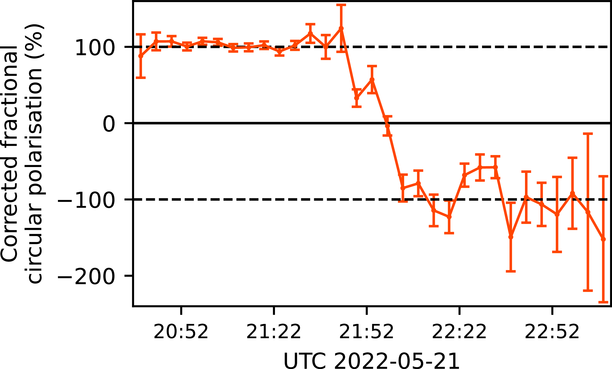
We analysed the fractional circular polarisation during the burst with the quiescent emission subtracted, computing
 \begin{equation} \frac {S_V - \bar {S}_{V,\text{qui}}}{S_I - \bar {S}_{I,\text{qui}}} \end{equation}
for each time bin during the burst. The result is shown in Figure 6. Both before and after the inversion, the burst had
 $\sim$
100% fractional circular polarisation, with a tighter constraint prior to the inversion due to the higher flux density. The bursts in Figure 2 were also
 $\sim$
100% circularly polarised. Such high fractional circular polarisation requires a coherent emission mechanism for the bursts.


3.4. Quiescent emission
Quiescent emission from M dwarfs is understood to originate from gyrosynchrotron radiation of mildly relativistic electrons with a power-law energy distribution (Kundu & Shevgaonkar Reference Kundu and Shevgaonkar1985) of spectral index
 $\delta \approx 3$
(White et al. Reference Whiting and Humphreys1989b). Assuming a magnetic field dependence
 $B \propto r^{-n}$
, where
 $r$
is the distance from a buried dipole at depth
 $r_0$
, and a collisionless plasma with density
 $N \propto r^{-m}$
, White et al. (Reference Whiting and Humphreys1989b) find the peak frequency of the quiescent emission to be
 \begin{equation} \small \frac {\nu _{\text{peak}}}{\mathrm{GHz}} = \left [ \frac {10^{2.72+0.33\delta } \frac {N_0}{10^{5}\,\mathrm{cm}^{-3}} \frac {r_0}{10^{9}\,\mathrm{cm}} } {m+n(0.30+0.98\delta )-1.00} \left ( \frac {B_0}{\mathrm{kG}} \right )^{0.30+0.98\delta } \right ]^\frac {1}{1.30+0.98\delta }. \end{equation}
Here,
 $N_0$
is the density of electrons with energies above a low-energy cutoff at the surface of the star and
 $B_0$
is the equatorial surface magnetic field.
Our ATCA observation showed the quiescent emission from WW PsA increased with frequency, implying high optical depth over the observed band, with
 $\nu _{\text{peak}} \gtrsim 3\,\mathrm{GHz}$
. In the case of a global dipolar magnetic field, i.e.
 $r_0 = R_\star = 0.70\pm 0.13\,{\rm R}_\odot$
(Messina et al. Reference Morin2017) and
 $n=3$
, taking typical values of the remaining parameters (
 $m=3$
,
 $\delta =3$
,
 $N_0 = 10^{5}\,\mathrm{cm^{-3}}$
) gives a loose lower bound on the field of
 $B_0 \gtrsim 200\,\mathrm{G}$
. Note that in Equation (3),
 $\nu _{\text{peak}}$
is much more strongly dependent on
 $B_0$
than the other variables, with the exception of
 $\delta$
. For example, increasing
 $N_0$
by a factor of 10 only reduces the lower bound on
 $B_0$
by a factor of 2. Setting
 $\delta = 2$
decreases the lower bound to
 $\sim \!70\,\mathrm{G}$
. However, White et al. (Reference Whiting and Humphreys1989b) find that models with
 $\delta = 2$
give flux densities much greater than those observed from real stars. Indeed, scaling the model flux densities in Tables 2, 3, and 5 of White et al. (Reference Whiting and Humphreys1989b) by a factor
 $(R_\star /10^{10}\,\mathrm{cm})^{2.46} (d/{2.7}\,\mathrm{pc})^{-2}\approx 0.8$
(using
 $S \sim r_0^{2.46}$
for optically thick emission with
 $\delta =2, m=n=3$
from Table 1 in the same work), the resulting flux densities at 1.5 GHz are much greater than that observed at this frequency in Figure 4. This confirms that
 $\delta \approx 3$
is a more realistic scenario for the quiescent emission from WW PsA. The bound
 $B_0 \gtrsim 200\,\mathrm{G}$
is unsurprising, as kG-scale average magnetic fields strengths have been measured from many M dwarfs (e.g. Kochukhov Reference Kochukhov and Lavail2021).
Among the observations from ASKAP in Figure 5, WW PsA was only detected in those with long durations (8–9 h). We posit this to be due to quiescent emission below the
 $\sim \!1\,\mathrm{mJy}$
detection thresholds for the observations with shorter durations. Note, however, that while Figure 3 and our follow-up observation confirm the presence of quiescent emission, we cannot exclude the possibility of these detections being caused by unpolarised bursts, except in the observations in which we produced Stokes
 $I$
dynamic spectra (see Table 1).
3.5. Coherent bursts
There are two mechanisms capable of producing the highly polarised coherent radio bursts we have observed from WW PsA: ECM emission and plasma emission. In this section, we calculate the magnetic field and plasma density required at the emission region in each scenario and discuss physical models which can explain the observed properties of the bursts.
ECM emission produces narrow-band emission close to harmonics of the local electron cyclotron frequency,Footnote f
 \begin{equation} \nu _{{c}} = \frac {eB}{2\pi m_{{e}} c} \end{equation}
where
 $e$
and
 $m_{{e}}$
are the charge and mass of the electron, respectively,
 $c$
is the speed of light, and
 $B$
is the local magnetic field strength at the emission site. Amplification is only expected to be significant for the first and second harmonics (Dulk Reference Freund, Czesla, Robrade, Schneider and Schmitt1985). The maser growth rate is greatest at the first harmonic, but the second harmonic is considered more likely to be observed due to strong gyroresonance absorption of the fundamental (Melrose & Dulk Reference Melrose and Dulk1982). If this is the emission mechanism, the observed frequency range of 891–1 137 MHz for the burst in Figure 3 implies a range of magnetic field strengths over the emission region of 320–410 G at the fundamental, or 160–200 G for emission at the second harmonic. In Figure 2, the emission covers 1 315–1 439 GHz, requiring magnetic field strengths of 470–510 G at the fundamental or 230–260 G at the second harmonic.
ECM emission is most efficient when
 $\nu _{{p}} \ll \nu _{{c}}$
(Melrose et al. Reference Messina1984), where
 \begin{equation} \nu _{{p}} = \sqrt {\frac {n_{{e}}e^2}{\pi m_{{e}}}} \end{equation}
is the electron plasma frequency and
 $n_{{e}}$
is the total number density of the electrons. For the radiation at
 $\nu = 891\,\mathrm{MHz}$
in Figure 3, this would imply
 $n_e \ll 9.8\times 10^{9}\,\mathrm{cm}^{-3}$
if
 $\nu \simeq \nu _c$
, or
 $n_e \ll 2.5\times 10^{9}\,\mathrm{cm}^{-3}$
if
 $\nu \simeq 2\nu _c$
.
Alternatively, if the observed bursts are due to plasma emission, their high fractional polarisation of
 $\sim$
100% can only be explained by emission at the fundamental of the plasma frequency (Dulk Reference Freund, Czesla, Robrade, Schneider and Schmitt1985). Thus, from Equation (5), the burst in Figure 3 would correspond to a range 0.98–
 $1.6\times 10^{10}\,\mathrm{cm}^{-3}$
of plasma densities over the emission region, while those in Figure 2 would correspond to 2.2–
 $2.6\times 10^{10}\,\mathrm{cm}^{-3}$
. These are in agreement with typical stellar coronal densities as measured from the X-ray O vii and Ne ix lines (Ness et al. Reference O’Brien, Keel, Hotan, Lenc, McConnell, Norris, Raja and Whiting2004).
The rate of detectable radio bursts from WW PsA is very low. The observations listed in Table 1 include 195.3 h covering the band 1 296.5–1 440.5 MHz, in which we detected two long-duration (
 ${\gtrsim} 30\,\mathrm{min}$
, adopting the terminology of Villadsen & Hallinan Reference Wang2019) circularly polarised bursts. Treating the bursts as stochastic for now and using a 95% Poisson confidence interval, we estimate they occur at a rate of
 $0.25^{+0.64}_{-0.22}\,\mathrm{d}^{-1}$
. That is, we expect there to be one burst detectable in Stokes
 $V$
for every
 $100^{+710}_{-70}\,\mathrm{h}$
of observation time in this band.
For comparison, Villadsen & Hallinan (Reference Wang2019) conducted observations of the M3V dwarf AD Leo, with 22 h covering the 1 296.5–1 440.5 MHz band. They detected three long-duration bursts in the relevant frequency range, each with maximum
 $S_V\gtrsim 5\,\mathrm{mJy}$
, well above our typical detection threshold. This yields one burst for every
 $7.3^{+28.2}_{-4.8}\,\mathrm{h}$
of observation time. A similar treatment for the observations of the M5.5V dwarf UV Cet in the same work implies one burst every
 $2.4^{+2.9}_{-1.2}\,\mathrm{h}$
(with a long-duration burst every
 $3.7^{+6.3}_{-2.0}\,\mathrm{h}$
). The higher measured burst rates of these stars compared to WW PsA can in part be attributed to their distances (
 $4.9651 \pm 0.0007\,\mathrm{pc}$
and
 $2.675 \pm 0.004\,\mathrm{pc}$
, respectively; Gaia Collaboration Reference Gary, Linsky and Dulk2023), as not all of the events reported by Villadsen & Hallinan (Reference Wang2019) would remain above our detection threshold when scaled to the distance of WW PsA. It may also be contributed to by physical differences such as the rotation period, which is much shorter for UV Cet, at
 $0.2268\pm 0.0003\,\mathrm{d}$
(Barnes et al. Reference Barnes, Jeffers, Haswell, Jones, Shulyak, Pavlenko and Jenkins2017), than for WW PsA.
The consistent absolute fractional polarisation of
 $\sim$
100% for all three bursts from WW PsA seen in Figures 2 and 6 is unusual behaviour for a magnetically active M dwarf. The coherent bursts from UV Cet, AD Leo (Villadsen & Hallinan Reference Wang2019), EV Lac (White et al. Reference White, Kundu and Jackson1989a; Osten et al. Reference Pallavicini, Willson and Lang2005; Lu et al. Reference Lynch, Lenc, Kaplan, Murphy and Anderson2025), and Proxima Centauri (Pérez-Torres et al. Reference Perley, Chandler, Butler and Wrobel2021; Zic et al. Reference Zic2020) mostly feature fractional polarisations below
 $\sim$
85%, and are consistent with 100% in only a small number of cases. However, in some cases this may be due to underlying quiescent emission, which we subtracted to produce Figure 6. All of these systems also produce short-duration bursts, which we did not detect from WW PsA.
Long-duration coherent radio bursts from M dwarfs have consistently been found to be due to ECM emission (Lynch et al. Reference McConnell2017; Villadsen & Hallinan Reference Wang2019; Bloot et al. Reference Bloot2024), so there is a strong possibility this is also the case for WW PsA. Evidence of ECM emission, rather than plasma emission, being the mechanism for a coherent burst can be found in a number of ways. These include, with varying levels of stringency:
-
1. identifying fine temporal structure (ms-timescale) in the dynamic spectrum (e.g. Osten & Bastian Reference Osten, Hawley, Allred, Johns-Krull and Roark2008);
-
2. combining the sense of the circular polarisation with information about the star’s magnetic field structure (e.g. from Zeeman Doppler imaging; Morin et al. Reference Murphy2008; Kochukhov & Lavail Reference Konijn2017; Villadsen & Hallinan Reference Wang2019) to determine if it is in the sense of the x-mode or the o-mode, which are favoured under typical conditions for ECM and plasma emission, respectively (Dulk Reference Freund, Czesla, Robrade, Schneider and Schmitt1985);
-
3. observing elliptical polarisation, which indicates the emission to be in the sense of the x-mode (Melrose & Dulk Reference Melrose, Dulk and Gary1991; Zic et al. Reference Zic2019); and
-
4. confirming the bursts are emitted in a highly beamed manner, particularly by identifying rotational modulation. Although plasma emission can be beamed tangentially to the magnetic field, as occurs in the case of some solar Type III radio bursts (Thejappa et al. Reference Thomas, Beuermann, Reinsch, Schwope, Truemper and Voges2012), narrow angular beaming is intrinsic to the ECM mechanism, making it the favourable explanation, especially when the emission is beamed at large angles to the magnetic field (e.g. Melrose & Dulk Reference Melrose and Dulk1982).
Given the available ASKAP observations have a time resolution of 10 s, that Zeeman Doppler imaging is unavailable, and because we did not detect linear polarisation, we are left with only rotational modulation as an avenue for finding direct evidence that the bursts from WW PsA are due to ECM emission. We investigate this possibility in the following sections.
3.5.1. Polarity reversal
Polarity reversal such as that shown in Figure 3 has been observed previously in rotationally modulated ECM emission at 154 MHz from UV Cet (Lynch et al. Reference McConnell2017). At 888 MHz, elliptically polarised bursts have been observed from UV Cet, indicating an auroral cavity with density more than six orders of magnitude lower than would otherwise be expected at the source altitude (Zic et al. Reference Zic2019).
An auroral oblique rotator model (e.g. Leto et al. Reference Leto2016) is therefore appropriate for UV Cet. Under this model, ECM emission is produced from auroral rings within cavities above each magnetic pole of the star, emitted in planes roughly perpendicular to the magnetic axis. Thus, a pair of pulses with opposite circular polarisation is observed near each magnetic null, that is, near the rotational phases at which the average line-of-sight stellar magnetic field is zero. The pulses may then be refracted in the stellar magnetosphere, increasing the delay between their arrival times. If the pulses are sufficiently separated, this results in an observed burst with polarity reversal at each magnetic null.
The strong dipolar magnetic field of UV Cet (Kochukhov & Lavail Reference Konijn2017) is consistent with this model. Rotationally modulated auroral ECM radiation of this type is well understood to be emitted by Earth, Jupiter, Saturn, Uranus, and Neptune (for a review, see Zarka Reference Zic1998). It has also been observed from some high-mass magnetic chemically peculiar (MCP) stars (e.g. Trigilio et al. Reference Villadsen and Hallinan2011; Das et al. Reference Das2024).
At frequencies above 744 MHz, the bursts from UV Cet have circular polarisation which is consistently right-handed (Villadsen & Hallinan Reference Wang2019; Zic et al. Reference Zic2019), whereas Lynch et al. (Reference McConnell2017) observed polarity reversals at 139–169 MHz. This behaviour is similar to our observation of polarity reversal in the bursts from WW PsA at lower frequencies (891–1 137 MHz), but not at higher frequencies (1 315–1 439 MHz). Likewise, in the case of the MCP stars HD 133880 and CU Vir, the oppositely polarised pulses are observed up to different maximum frequencies (Das et al. Reference Das, Chandra and Wade2020; Das & Chandra Reference Das, Chandra and Petit2021). This may be due to asymmetry in the magnetic field or the magnetosphere (Das & Chandra Reference Das, Chandra and Petit2021).
Polarity reversal has also been observed in bursts of rotationally modulated ECM emission from the ultracool dwarfs TVLM 513
 $-$
46546 (Hallinan et al. Reference Hallinan2007; Lynch et al. Reference Lynch, Mutel and Güdel2015) and 2MASS J0746425
 $+$
200032 (Lynch et al. Reference Lynch, Mutel and Güdel2015). In both cases, Lynch et al. (Reference Lynch, Mutel and Güdel2015) found that the observed dynamic spectra are much better explained by a sequence of three distinct emission sites, corresponding to separate coronal loops. Thus, rotational modulation does not necessarily require the emission to be auroral in nature. This means that although auroral emission is perhaps the simplest geometric model that can explain the observed polarity reversal from WW PsA, it is not the only plausible explanation, even in the case of rotationally modulated bursts of ECM emission. However, any geometric model for the polarity reversal must rely on narrow angular beaming, which is more easily explained by ECM emission than plasma emission.
Alternatively, the polarity reversal may be caused by a change in the dominant magneto-ionic mode emitted due to variations in the properties of the plasma in the emission region. For example, consider the case of emission from a cyclotron maser driven by a loss cone. The growth rates of the modes are strongly dependent on the ratio
 $\nu _{{p}}/\nu _{{c}}$
, with the fundamental x-mode becoming suppressed for
 $\nu _{{p}}/\nu _{{c}} \gtrsim 0.3$
(Melrose et al. Reference Messina1984). A rapid change in
 $n_{{e}}$
or
 $B$
could cause the dominant mode to change from the x-mode to the o-mode, or vice versa, resulting in the polarity reversal seen in Figure 3. Significant ECM emission in the sense of the o-mode is known to be possible under stellar conditions, as it has been observed from the early-type star HD 142301 (Leto et al. Reference Lin, Apai, Giampapa and Ip2019). With the parameters considered by Sharma & Vlahos (Reference Shkolnik, Anglada-Escudé, Liu, Bowler, Weinberger, Boss, Reid and Tamura1984), for a saturated maser the predicted polarisation fraction transitions sharply from 100% in the sense of the x-mode to 100% in the sense of the o-mode at
 $\nu _{{p}}/\nu _{{c}} = 0.35$
. Under such conditions, a transition from, say,
 $\nu _{{p}}/\nu _{{c}} = 0.33$
to
 $0.37$
(e.g. due to a
 $\sim$
25% increase in
 $n_{{e}}$
or a
 $\sim$
10% decrease in
 $B$
) over the course of
 $\sim \!20\,\mathrm{min}$
could therefore explain the behaviour of the fractional polarisation shown in Figure 6. The power emitted in the x-mode when it is dominant is expected to be greater than that in the o-mode when it is dominant (Sharma & Vlahos Reference Shkolnik, Anglada-Escudé, Liu, Bowler, Weinberger, Boss, Reid and Tamura1984). Thus, in this scenario, we suggest that the higher flux density prior to the polarity reversal (see Figure 3) is in better agreement with a transition from the x-mode to the o-mode than vice versa, i.e. an increase in
 $n_{{e}}$
or a decrease in
 $B$
.
However, in the case of plasma emission, such a transition in the dominant magneto-ionic mode cannot explain the behaviour of the fractional polarisation in Figure 6. This is because fundamental plasma emission occurs below the right-hand cut-off of the x-mode (Dulk Reference Freund, Czesla, Robrade, Schneider and Schmitt1985; Chen Reference Chen2016),
 \begin{equation} \nu _{{R}} = \frac {1}{2} \left ( \nu _{{c}} + \sqrt {\nu _{{c}}^2 + 4\nu _{{p}}^2} \right ) \gt \nu _{{p}}, \end{equation}
so the emission can only be in the sense of the o-mode,Footnote g while at the second harmonic the radiation is not expected to have such high fractional polarisation (e.g. Melrose et al. Reference Melrose, Dulk and Smerd1978, Reference Melrose, Hewitt and Dulk1980; Dulk Reference Freund, Czesla, Robrade, Schneider and Schmitt1985).
3.5.2. Rotational modulation
We investigated the possibility that the observed bursts from WW PsA were rotationally modulated. We used the photometric rotation period
 $P_{\text{rot}} = 2.356 \pm 0.001\,\mathrm{d}$
determined by Ibañez Bustos et al. (Reference Jayawardhana, Coffey, Scholz, Brandeker and van Kerkwijk2023) with data from the Transiting Exoplanet Survey Satellite (TESS; Ricker et al. Reference Rose2015). However, we note that the uncertainty in this measurement does not account for the effect of differential rotation of starspots (e.g. Collier Cameron Reference Collier Cameron2002), so the results following from it are tentative. For sufficient
 $N \in \mathbb{Z}$
we calculated the Barycentric Julian Dates (BJDs)
 \begin{equation} \text{BJD}_N = \text{BJD}_0 + NP_{\text{rot}}, \end{equation}
corresponding to the same rotational phase
 $\phi _0$
as the centre of the burst in Figure 3, at time
 $\mathrm{BJD}_0 = 2\,459\, 721.410(7)\mathrm{d}$
. We compared these to the BJDs of the bursts in Figure 2: 2 460 554.00–2 460 554.07 d for the earlier burst and 2 460 581.28–2 460 581.31 d for the later burst. Doing so, we found
 $\text{BJD}_{365} = 2\,460\,581.35(37)\,\mathrm{d}$
to be consistent with the time of the later burst, whereas the earlier burst was closest to
 $\text{BJD}_{353} = {2\,460\,553.08(35)}\,\mathrm{d}$
, offset from its centre by
 $2.7\sigma _{\text{BJD}_{353}}$
. The later burst can therefore plausibly be explained by rotationally modulated pulses from the same emission region as that for the burst in Figure 3, but this is unlikely for the earlier burst.
If the emission is rotationally modulated, it is possible to place further constraints on the properties of the star. We denote our updated quantities with a prime. Enforcing
 $\text{BJD}_{365}' = \text{BJD}_{\text{later}} = {2\,460\,581.30(2)}\,\mathrm{d}$
, where
 $\text{BJD}_{\text{later}}$
is the BJD of the later burst in Figure 2 (covering the possibility that its end corresponds to the end of the centre of the burst in Figure 3), we consider a new ephemeris,
 \begin{equation} \text{BJD}_N' = \text{BJD}_0 + NP_{\text{rot}}', \end{equation}
to obtain
 $P_{\text{rot}}' = 2.355\,86(6)\,\mathrm{d}$
. We work with this rotation period moving forward, but caution that it is both model-dependent and reliant on the optical period reported by Ibañez Bustos et al. (Reference Jayawardhana, Coffey, Scholz, Brandeker and van Kerkwijk2023). Next, we adopt the projected rotational velocity
 $v \sin i = 12.0\pm 1.1\,\mathrm{km\,s}^{-1}$
, which Messina et al. (Reference Morin2017) infer from prior work (Christian & Mathioudakis Reference Christian and Mathioudakis2002; Torres et al. Reference Treumann2006; Jayawardhana et al. Reference Johnstone and Güdel2006; Bailey et al. Reference Bailey, White, Blake, Charbonneau, Barman, Tanner and Torres2012), where
 $i$
is the inclination of the rotation axis to the line of sight. Then,
 \begin{equation} \sin i' = \frac {P_{\text{rot}}'}{2 \pi R_\star } \left ( v \sin i \right ) \end{equation}
gives
 $\sin i' = \text{0.80} \pm \text{0.17}$
, or
 $i' = \text{53}^{+\text{22}}_{-\text{14}}$
deg. This does not improve the precision of the measured inclination compared to that found by Messina et al. (Reference Morin2017), as the dominant sources of uncertainty are
 $v \sin i$
and
 $R_\star$
.
The burst on 2025–09–13 (see Section 2.2) had a BJD range spanning from 2 460 932.19 d to at least 2 460 932.39 d. This matches
 $\text{BJD}_{514}' = 2\,460\,932.32(3)\,\mathrm{d}$
from Equation (8). Using an alternative ephemeris given by
 \begin{equation} \text{BJD}_M = \text{BJD}_{\text{later}} + MP_{\text{rot}}, \end{equation}
where
 $M \in \mathbb{Z}$
, yields
 $\text{BJD}_{M=149} = 2\,460\,932.34(15)\,\mathrm{d}$
. With either method, the arrival time of the burst on 2025–09–13 is successfully predicted. We therefore tentatively claim that the bursts are composed of rotationally modulated pulses. This is most easily explained by the intrinsic narrow angular beaming of ECM emission.
The earlier burst in Figure 2, at time
 $\text{BJD}_{\text{earlier}} = 2\,460\,554.04(4)\,\mathrm{d}$
, differs in phase from the later burst (and thus also the burst in Figure 3) according to
 \begin{equation} \Delta \phi = \left \{ \frac {\text{BJD}_{\text{earlier}} - \text{BJD}_{\text{later}}}{P_{\text{rot}}'} \right \}, \end{equation}
where
 $\{x\} = x- \lfloor x \rfloor$
denotes the fractional part of
 $x$
. We obtain
 $\Delta \phi = \text{0.429} \pm \text{0.019}$
.
Among the observations listed in Table 1, the ephemeris given by Equation (8) predicts bursts in the ASKAP scheduling blocks SB65347 for
 $N=353$
, SB65665 for
 $N=356$
, and SB65818 for
 $N=359$
. Additionally, if the earlier burst in Figure 2 is also rotationally modulated, we expect bursts at the times
 $\text{BJD}_0 + (N+\Delta \phi )P_{\text{rot}}'$
. We therefore also predict bursts in SB40196 for
 $N=-8$
, SB40880 for
 $N=0$
, and SB65836 for
 $N=359$
. However, we did not detect polarised emission in any of these observations. If the emission is rotationally modulated, this may be due to intrinsic variability between pulses caused by instability in the emission region, which occurs, for example, in the case of the ECM pulses from CU Vir (e.g. Ravi et al. Reference Rhee2010). Trigilio et al. (Reference Villadsen and Hallinan2011) note that the ECM growth rate is a nonlinear function of various parameters (e.g. Melrose et al. Reference Messina1984; Sharma & Vlahos Reference Shkolnik, Anglada-Escudé, Liu, Bowler, Weinberger, Boss, Reid and Tamura1984; Mutel et al. Reference Myserlis2007), including
 $n_{{e}}$
and
 $B$
, as well as the electron velocity distribution and its anisotropy. Small variations in these parameters can therefore cause the large variations in the observed flux density. In addition, ECM emission requires acceleration or heating of electrons, for example resulting from magnetic field reconnection (Dulk Reference Freund, Czesla, Robrade, Schneider and Schmitt1985). It may be that the observed bursts were enabled by such events. Magnetic reconnection is also responsible for stellar flares (e.g. Parker Reference Pérez-Torres1963), several of which have been identified from WW PsA (Ibañez Bustos et al. Reference Jayawardhana, Coffey, Scholz, Brandeker and van Kerkwijk2023; Lin et al. Reference Lourenço2024) in observations from TESS.
3.5.3. Oblique rotator model
For an oblique rotator model (e.g. Leto et al. Reference Leto2016), in which the bursts are auroral and the star has a dipolar field, there is a magnetic null at
 $\phi _0$
. Then, taking the earlier burst in Figure 2 to be at the other null and choosing the phases such that it occurs at
 $1-\phi _0$
gives
 $\phi _0 = (1-\Delta \phi )/2 = \text{0.286} \pm \text{0.009}$
. Radiation emitted at an angle
 $\theta _{\text{M}}$
to the magnetic dipole axis is observed at phase
 $\phi$
, where (Trigilio et al. Reference Trigilio, Leto, Umana, Buemi and Leone2000; Leto et al. Reference Leto2016)
 \begin{equation} \cos \theta _{\text{M}} = \sin \beta \sin i' \cos 2\pi \phi + \cos \beta \cos i'. \end{equation}
The obliquity
 $\beta$
is the angle between the rotation axis and the magnetic dipole axis. The magnetic nulls correspond to
 $\cos \theta _{\text{M}} = 0$
, implying (Leto et al. Reference Leto2016)
 \begin{equation} \beta = \arctan \left (\frac {-1}{\tan i' \cos 2\pi \phi _0}\right ). \end{equation}
This yields
 $\tan \beta = \text{3.4} \pm \text{2.1}$
, or
 $\beta = \text{74}^{+\text{6}}_{-\text{22}}\,\mathrm{deg}$
. Such a high obliquity would be unusual for a star of type
 $\sim \!\text{M4}$
. Among those investigated by Morin et al. (Reference Murphy2008), most featured fields with strong dipolar components closely aligned with the rotation axis (i.e. low
 $\beta$
), with the exception of EV Lac, which had the longest rotation period of 4.38 d (compared to 0.40–2.77 d for the other five stars). We note that these stars have masses in the range 0.25–0.42
 ${\rm M}_\odot$
, higher than that of WW PsA at
 $0.19\pm 0.04\,{\rm M}_\odot$
(Messina et al. Reference Morin2017).
We can now determine the range of angles
 $\theta _{\text{M}}$
which the burst in Figure 3 corresponds to under the oblique rotator model. The right circularly polarised (RCP) and left circularly polarised (LCP) pulses lasted
 ${\sim} {1.3 \,\mathrm{h}}$
prior to and after the null at
 $\phi _0$
, respectively. Substituting the corresponding range of phases into Equation (12), we find that the start of the RCP pulse corresponds to
 $\theta _{\text{M}} = {83.8 \pm 3.8}\,\mathrm{deg}$
, while the end of the LCP pulse corresponds to
 $\theta _{\text{M}} = 96.0\pm 3.8\,\mathrm{deg}$
. That is, the maximum upward deflection of the radiation from the plane perpendicular to the dipole axis was
 $6.2 \pm 3.8\,\mathrm{deg}$
for the RCP pulse and
 $6.0\pm 3.8\,\mathrm{deg}$
for the LCP pulse.
3.5.4. Pulse spectral properties
For the dynamic spectra in Figure 3, we performed a linear transformation from the Stokes
 $I$
and
 $V$
flux densities to those of the RCP and LCP components of the field,Footnote
h
 \begin{equation} S_{\text{RCP}} = \frac {S_I + S_V}{2} \end{equation}
and
 \begin{equation} S_{\text{LCP}} = \frac {S_I - S_V}{2}. \end{equation}
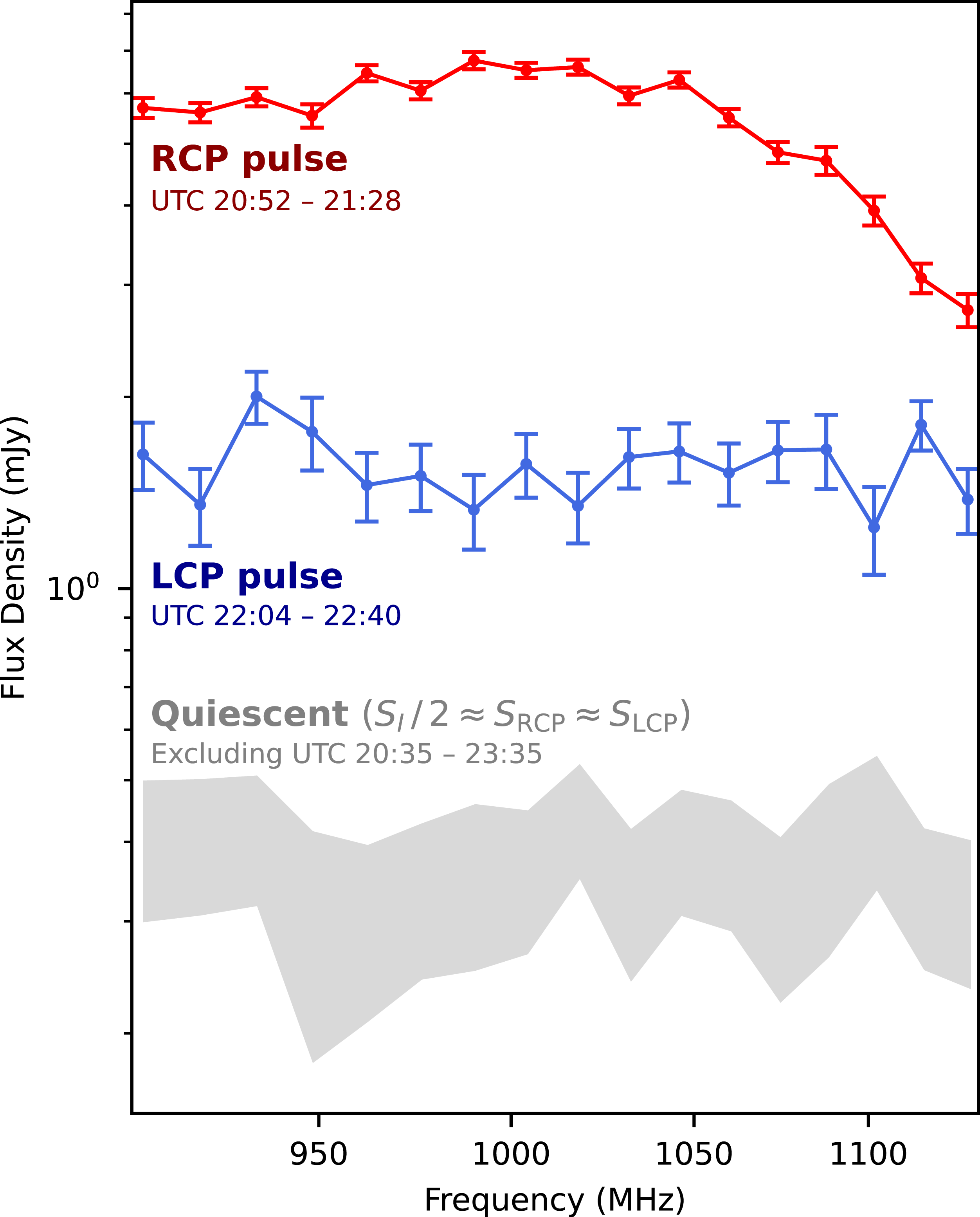
This allowed us to separate the RCP and LCP pulses. At the peak of each pulse (2022–05–21 20:52 to 21:28 UTC for the RCP pulse and 22:04 to 22:40 UTC for the LCP pulse) we created a spectrum, shown in Figure 7. Also shown in Figure 7 is the spectrum of the quiescent emission in the same observation, where we have used
 $S_I/2$
to estimate
 $S_{\text{RCP}}$
and
 $S_{\text{LCP}}$
given its low fractional polarisation, as discussed in Section 3.3.
Spectra of
 $S_{\text{RCP}}$
and
 $S_{\text{LCP}}$
at the peaks of the RCP and LCP pulses, respectively, for the burst shown in Figure 3. Also shown is the spectrum of the quiescent emission, for which we use
 $S_I / 2$
to estimate both
 $S_{\text{RCP}}$
and
 $S_{\text{LCP}}$
. The grey band indicates the range
 $S_I / 2 \pm \sqrt {\sigma _{S_I/2}^2 + \sigma _{S_V/2}^2}$
. All times shown are for the date 2022–05–21 UTC. For the quiescent emission, the whole observation was included except the period indicated.

The quiescent emission did not show significant variation over the observed bandwidth. The RCP pulse behaved similarly to the auroral pulses emitted by some MCP stars (e.g. Das & Chandra Reference Das, Chandra and Petit2021), featuring a roughly constant flux density followed by a decrease beginning at
 ${\sim} 1\,050\,\mathrm{MHz}$
. By fitting a power law for the latter part of the spectrum, we estimated the RCP pulse should merge with the
 $\sim \!0.4\,\mathrm{mJy}$
level of the quiescent emission at 1 300–1 400 MHz. The LCP pulse did not exhibit the same behaviour, remaining approximately constant over the band.
4. Summary
In this work we have identified coherent radio bursts and quiescent emission from WW PsA. This resulted from a
 $2.2\times 10^{4}$
star-hour volume-limited search for polarised stellar radio emission in the ASKAP DINGO survey. For WW PsA, we searched for polarised bursts in the dynamic spectra and lightcurves from 283.3 h of observations. We detected three bursts in this search, with a fourth identified in a later DINGO observation with the VASTER pipeline.
The quiescent emission varied slowly on a timescale of hours. As we found its peak frequency to be
 ${\gtrsim} 3\,\mathrm{GHz}$
, we expect the surface magnetic field at the relevant sites of emission to be in the hundreds of gauss.
One of the bursts exhibited polarity reversal, a common feature of rotationally modulated ECM emission. We found the bursts to be consistent with rotationally modulated emission given the photometric rotation period reported by Ibañez Bustos et al. (Reference Jayawardhana, Coffey, Scholz, Brandeker and van Kerkwijk2023). Using the radio bursts, we derived an updated rotation period
 $P_{\text{rot}}' = {2.355\,86 \pm 0.000\,06}\,\mathrm{d}$
and inclination
 $i' = 53^{+22}_{-14}\,\mathrm{deg}$
. Under an oblique rotator model, we also derived the obliquity
 $\beta = 74^{+6}_{-22}\,\mathrm{d}$
and the maximum upward deflection angles of
 $6.2\pm 3.8\,\mathrm{deg}$
and
 $6.0\pm 3.8\,\mathrm{deg}$
for the RCP and LCP pulses, respectively. The required narrow angular beaming suggests ECM emission as the most likely mechanism if the bursts are rotationally modulated. For second harmonic ECM emission, the observed frequency ranges require field strengths at the emission sites of 160–200 G and 230–260 G. Our ephemeris predicts burst arrival times during some observations in which we made no detection, which may be due to a variable maser growth rate caused by changing conditions in the plasma, also seen in the auroral ECM pulses from MCP stars. One of the observed pulses from WW PsA also shows similar spectral behaviour to pulses from MCP stars.
Under an alternative model in which the polarity reversal is due to a change in the dominant magneto-ionic mode of the emission, we still favour the ECM mechanism. This is because plasma emission cannot explain a polarity reversal from 100% fractional polarisation in the sense of one mode to 100% in the sense of the opposite mode.
Acknowledgements
We thank the reviewer for their suggestions regarding our discussion of physical models for the bursts from WW PsA.
JM-B is supported by an Australian Government Research Training Program (RTP) Scholarship.
Parts of this research were supported by the Australian Research Council Centre of Excellence for Gravitational Wave Discovery (OzGrav), project number CE230100016.
This scientific work uses data obtained from Inyarrimanha Ilgari Bundara, the CSIRO Murchison Radio-astronomy Observatory. We acknowledge the Wajarri Yamaji People as the Traditional Owners and native title holders of the Observatory site. CSIRO’s ASKAP radio telescope is part of the Australia Telescope National Facility (https://ror.org/05qajvd42). Operation of ASKAP is funded by the Australian Government with support from the National Collaborative Research Infrastructure Strategy. ASKAP uses the resources of the Pawsey Supercomputing Research Centre. Establishment of ASKAP, Inyarrimanha Ilgari Bundara, the CSIRO Murchison Radio-astronomy Observatory and the Pawsey Supercomputing Research Centre are initiatives of the Australian Government, with support from the Government of Western Australia and the Science and Industry Endowment Fund.
The Australia Telescope Compact Array is part of the Australia Telescope National Facility (https://ror.org/05qajvd42) which is funded by the Australian Government for operation as a National Facility managed by CSIRO. We acknowledge the Gomeroi people as the Traditional Owners of the Observatory site.
This paper includes archived data obtained through the CSIRO ASKAP Science Data Archive, CASDA (http://data.csiro.au).
The National Radio Astronomy Observatory and Green Bank Observatory are facilities of the U.S. National Science Foundation operated under cooperative agreement by Associated Universities, Inc.
Data availability statement
The ASKAP data used in this paper are public and can be accessed through the CSIRO ASKAP Science Data Archive (CASDAFootnote i ) under project codes AS032, AS034, AS104, AS110, AS115, AS204, and AS207. The ATCA data and subsequent analysis are available upon request. The VLASS Quick Look catalogues used are publicly available from the Canadian Initiative for Radio Astronomy Data Analysis (CIRADA) website.Footnote j


 I

 I
 V
 I
 V

 I
 V
 I
 Q
 U
 V
 I

 I
 σrms
 5σrms
 σrms
 I
 V
 SRCP
 SLCP
 SI/2
 SRCP
 SLCP
 SI/2±σSI/22+σSV/22

 Open access

