1. INTRODUCTION
Seamless navigation in challenging Global Navigation Satellite System (GNSS) environments is of great importance for land vehicle navigation. Alternative sensors (e.g. Inertial Measurement Units - IMU) are usually used to bridge GNSS outages. An IMU is a self-contained sensor, which integrates rotation rates to obtain orientation changes, and doubly integrates the accelerations to obtain velocity and position increments (Jekeli, Reference Jekeli2001). However, IMU output errors accumulate with time, resulting in degraded performance, especially for low-cost Micro-Electro-Mechanical System (MEMS)-based IMUs. Stereo Visual Odometry (VO) is another widely applied Dead-Reckoning (DR) approach which utilises continuously tracked features in consecutive frames to estimate the camera pose. Similar to GNSS/Inertial Navigation System (INS) integration, which is widely applied to increase the reliability and continuity of the system, INS/Stereo VO integration can also mitigate the quick drift of a stand-alone INS or stereo VO.
Since both stereo VO and IMU can provide navigation solutions individually, they can be integrated in a loosely coupled way in which each individual system is processed separately and the outputs from each system are fused by a Kalman filter (Tardif et al., Reference Tardif, George, Laverne, Kelly and Stentz2010; Konolige et al., Reference Konolige, Agrawal and Sola2010). Although the loosely coupled integration can limit the quick drift of each individual sensor, the measurement information from each system cannot be fully applied (Grewal et al., Reference Grewal, Weill and Andrews2007). In contrast, tight integration utilises only one single centralised Kalman filter where the raw measurements of sensors are directly used. Many studies have been made on tight integration of INS and stereo VO (Asadi and Bottasso, Reference Asadi and Bottasso2014; Strelow, Reference Strelow2004; Veth and Raquet, Reference Veth and Raquet2007; Liu et al., Reference Liu, Sarvrood and Gao2015; Carrillo et al., Reference Carrillo, López, Lozano and Pégard2012; Usenko et al., Reference Usenko, Engel, Stückler and Cremers2016; Xian et al., Reference Xian, Hu and Lian2015). However, these studies have provided few details of how a tight integration is conducted and implemented including the derivation of related mathematical equations, especially the system implementation at a local-level frame using the conventional INS 15-parameter error model. If a conventional INS 15-parameter error model is used, the formulation of the design matrix for the measurement model is a challenge although the process model in Kalman filters has been well developed. In this paper, we develop the system models and equations necessary for the implementation of an integrated inertial visual odometry system. This includes details of how pixel measurements from visual odometry can be applied directly to correct the inertial sensor errors and the derivation of all involved matrices in the Extended Kalman Filter (EKF). The effectiveness of the tight integration implementation is demonstrated by field tests. In addition to position estimation, the velocity and azimuth solutions from the integrated system also outperform a stand-alone INS or stereo VO system.
2. RELATED WORKS
A considerable number of studies have discussed the integration of inertial and stereo visual datasets. For loose integration of INS/Stereo VO, one common method is to apply the rotation and translation estimated by visual odometry to correct the mechanisation results obtained by inertial datasets (Tardif et al., Reference Tardif, George, Laverne, Kelly and Stentz2010). Similarly, the inertial measurements of an IMU could also be used to correct the ego-motion estimation by visual odometry (Konolige et al., Reference Konolige, Agrawal and Sola2010). To fully employ the measurement information of each type of sensor, tight integration of INS and stereo VO has been explored by many researchers. Strelow (Reference Strelow2004) and Carrillo et al. (Reference Carrillo, López, Lozano and Pégard2012) used both acceleration and rotation measurements in an IMU body frame and pixel coordinates in images to correct motion under certain assumptions. Soloviev and Miller (Reference Soloviev and Miller2012) proposed a generic multi-sensor fusion approach which builds the navigation mechanisation around a self-contained IMU as a core sensor. Externally-dependent sources of navigation information are treated as secondary sensors, whose measurements are utilised to reduce drift in inertial navigation outputs. In other words, in this architecture, dynamic information is provided by the inertial sensors while the pixel coordinates are the measurement update to correct inertial sensor errors. Within such an architecture, Bottasso et al. (Reference Bottasso, Leonello and Milano2008) employed inertial data to initialise the motion of a platform instead of assuming a certain motion model. In this implementation, feature positions are estimated in the filter, which may increase the filter failure probability due to complex state vector settings. Veth and Raquet (Reference Veth and Raquet2007) filtered out stale features whose tracking are lost for a given period to simplify the data association. Asadi and Bottasso (Reference Asadi and Bottasso2014) summarised existing tightly coupled stereo vision-aided inertial navigation methods. Xian et al. (Reference Xian, Hu and Lian2015) discussed the impact of features at different distances and Kong et al. (Reference Kong, Wu, Zhang and Wang2015) utilised line measurements away from point features. Usenko et al. (Reference Usenko, Engel, Stückler and Cremers2016) excluded the feature position in the state vector. Most of these works focus on implementation in a self-defined local frame. Conventional INS error models in local-level frames have rarely been used in previous implementations. Liu et al. (Reference Liu, Sarvrood and Gao2015) proposed the implementation architecture of a tightly coupled integration of INS/Stereo VO formed in a local-level frame for land vehicle navigation. However, these studies rarely provided the details of a tight integration implementation procedure using the conventional INS 15-parameter error model.
3. METHODOLOGY
This section describes the method of applying pixel measurements to correct inertial sensor errors. Before introducing the tight integration procedures in Section 3.3, fundamental equations in stereo visual odometry and inertial navigation are first reviewed in Sections 3.1 and 3.2, which are necessary for tight integration.
3.1. Formulation of Stereo VO
There are generally three main steps in visual odometry. The first step is to detect and match the image correspondences over consecutive epochs. Well-developed matching and tracking algorithms can be applied to find the correspondences (Tomasi and Kanade, Reference Tomasi and Kanade1991; Lowe, Reference Lowe2004). The second step of VO is motion estimation, which generally can be summarised as three approaches, namely Two Dimensional (2D) to 2D, Three-Dimensional (3D) to 3D and 3D to 2D (Scaramuzza and Fraundorfer, Reference Scaramuzza and Fraundorfer2011). The last step in visual odometry is to optimise the estimated results with methods such as bundle adjustment. In this work, the last step is not necessary because an integration with an IMU is conducted.
The first motion estimation method from 2D to 2D uses a certain number of matched features in two consecutive epochs to compute the essential matrix, from which the rotation and translation can be decomposed up to a scale ambiguity. Then, the translation vector needs to be rescaled. This has been explored by Hartley and Zisserman (Reference Hartley and Zisserman2003) and Nistér (Reference Nistér2004). The 3D to 3D method is more straightforward, where two sets of 3D coordinates are triangulated by two pairs of stereo images, and the rotation and translation can be computed from these two sets of points (Pankaj and Nidamanuri, Reference Pankaj and Nidamanuri2016). The 3D to 2D method is the most frequently applied in visual odometry due to higher accuracy and easier data association (Nistér et al., Reference Nistér, Naroditsky and Bergen2004). In this method, the optimal rotation and translation are computed based on minimising the re-projection errors of the 3D features, which are obtained by triangulation of a previous pair of images, on the current image as shown in the equation below.
 $$\arg \min_{T_k} \sum \Vert p_k^i - \hat{p}_k^i \Vert ^2$$
where
 $p_{k}^{i}$
are the feature image coordinates and
 $\hat{p}_{k}^{i}$
is the re-projection of the features on the current image according to the rotation and translation. This is known as Perspective from n Points (PnP) (Kneip et al., Reference Kneip, Scaramuzza and Siegwart2011; Lepetit et al., Reference Lepetit, Moreno-Noguer and Fua2009; Hartley and Zisserman, Reference Hartley and Zisserman2003). A least squares adjustment is applied to solve PnP. After obtaining the rotation and translation between two consecutive epochs, the current pose with respect to the initial point can be achieved by accumulating the rotation and translation.
In this work, the computation of rotation and translation by PnP is not necessary in the integration with IMU. Only the re-projection of features is conducted in the integration, which is based on feature coordinates, camera position and attitude obtained by the mechanisation of the IMU. The mechanisation of the IMU is conducted in a Local-Level Frame (LLF), which means that the position has to be transformed to a Cartesian coordinate system. We set the left camera frame at the first epoch as the world frame, which is the Cartesian coordinate system required. In other words, the feature coordinates are obtained by triangulation, the camera rotation and translation are expressed in the world frame. As mentioned before, the prediction of pixel coordinates of features is differenced with measured coordinates to form the measurement update in an EKF. Therefore, the re-projection is one important step in this work. The 3D feature coordinates in the world frame have to be transformed to the current left camera frame, given as
 $$\left[\matrix{X_c & Y_c & Z_c} \right]^{T} = [R \vert t] \left[\matrix{ X_w & Y_w & Z_w &1 } \right]^T$$
where R and t represent the rotation and translation of the feature coordinates from the world frame to the current left camera frame. This can be obtained from the mechanisation results of the IMU. X w , Y w and Z w represent the 3D coordinates of features in the world frame and X c , Y c and Z c represent the 3D coordinates of features in the current left camera frame. The calibrated and rectified images are used and the perspective camera model is assumed as a pin-hole projection system given as
 $$\left[\matrix{ x \cr y \cr z } \right] = \left[\matrix{ f_x &0 & u_0 \cr 0 & f_y & v_0 \cr 0 &0 &1 } \right] \left[\matrix{ X_c \cr Y_c \cr Z_c} \right] \left[\matrix{ u \cr v } \right] = \left[\matrix{ x/z \cr y/z } \right]$$
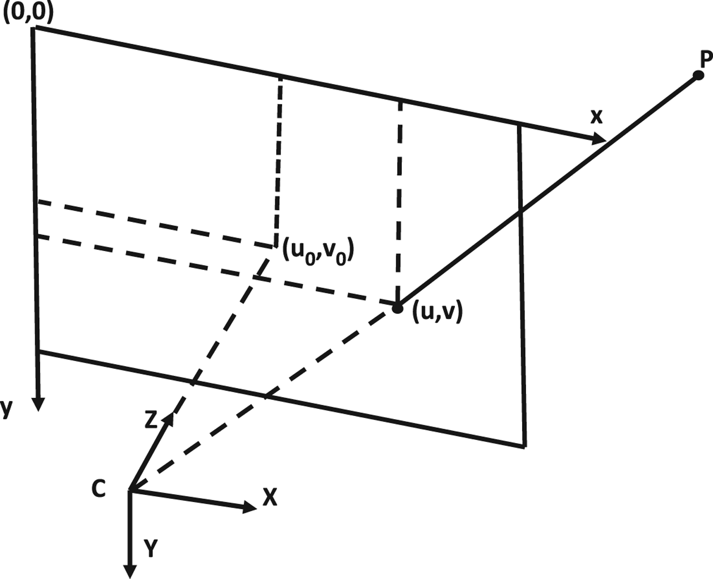
where X c , Y c and Z c are the feature coordinates in the camera frame, f x , f y are the focal length of each image axis, u 0 and v 0 are the projection of perspective centre coordinates on the image and u and v are the pixel coordinates of features in the image. The camera frame is defined as right, down and forward while the axes of the image frame are pointing to right and down with the left up corner as the origin. The camera and image frames are illustrated in Figure 1.
Projection of features on image.

3.2. Inertial Navigation Fundamental Equations
The tightly coupled architecture is based on the dynamics information provided by the IMU. The equations of mechanisation and the INS error models are reviewed in this section. In this paper, the IMU body frame is defined as right, forward and up while the LLF is defined as East, North and Up (ENU). According to Noureldin et al. (Reference Noureldin, Karamat and Georgy2012), the mechanisation equations can be formed as
 $$\left[\matrix{ \dot{r}^l \cr \dot{V}^l \cr \dot{R}_l^b } \right] = \left[\matrix{ D^{-1} V^l \cr R_b^l f^b - \lpar 2\Omega_{ie}^l + \Omega_{ie}^l \rpar V^l + g^l \cr R_b^l \lpar \Omega_{ib}^b + \Omega_{il}^l \rpar } \right]$$
where
 $\dot{r}^{l}$
,
 $\dot{V}^{l}$
and
 $\dot{R}_{l}^{b}$
represent the time derivatives of position, velocity and rotation matrix respectively, and the superscript ‘l’ and ‘b’ represent the local-level frame and the IMU body frame,
 $R_{b}^{l}$
is the rotation matrix from the IMU body frame to the local-level frame,
 $\Omega_{ab}^{c}$
is the skew-symmetric matrix of the rotation rate
 $\omega_{ab}^{c}$
, which represents the rotation rate from frame ‘b’ relative to frame ‘a’ expressed in frame ‘c’, f
b
is the acceleration measured by the IMU in its body frame,
 $\omega_{ib}^{b}$
is the angular rate vector sensed by the gyroscope triad,
 $\omega_{ie}^{l}$
and
 $\omega_{el}^{l}$
are the earth rotation rate projected in the local-level frame and the transport rate caused by the change of orientation of the local-level frame respectively and
 $\omega_{il}^{l}$
is the sum of the
 $\omega_{ie}^{l}$
and
 $\omega_{el}^{l}$
. Moreover, the first equation of Equation (4) represents the relationship between the geographic coordinates and the velocity components in the local-level frame, given by
 $$\eqalign{r^l &= \left[\matrix{ \varphi &\lambda & h } \right]^T \cr D^{-1} &= \left[\matrix{ 0 &{1 \over R_m + h} &0 \cr {1 \over \lpar R_n + h\rpar \cos \varphi} &0 &0 \cr 0 &0 &1 } \right] \cr V^l &= \left[\matrix{ V_e & V_n & V_u } \right]^T}$$
with R
m
and R
n
representing the meridian radius of curvature and the radius of curvature of the prime vertical respectively,
 $\varphi, \lambda, h$
representing latitude, longitude and height respectively and V
e
, V
n
and V
u
representing the velocity in east, north and up directions in the LLF.
The initial rotation matrix
 $R_{b}^{l}$
can be achieved by multiplying an elementary rotation matrix with known attitude angles, given as
 $$\eqalign{R_b^l &= R_3 (yaw) R_1 (pitch) R_2 (roll) \cr &= \left[\matrix{ \cos y &-\sin y &0 \cr \sin y &\cos y &0 \cr 0 &0 &1 } \right] \left[\matrix{ 1 &0 &0 \cr 0 &\cos p &-\sin p \cr 0 &\sin p &\cos p } \right] \left[\matrix{ \cos r &0 &\sin r \cr 1 &0 &0 \cr -\sin r &0 &\cos r \cr } \right]}$$
where y presents yaw, p is pitch and r is roll. The rotation matrix can be updated by applying the third equation of Equation (4). With the updated rotation matrix
 $R_{b}^{l}$
, a vector can be transformed from the IMU body frame to the LLF, which indicates that the acceleration sensed by the IMU in the body frame can be transformed into the LLF. However, the IMU acceleration measurements contain not only the acceleration of the platform, but also the local gravity, the Coriolis force of earth rotation and the influence caused by the change of orientation of the local-level frame, which all need to be removed. This explains the second equation in Equation (4). After updating the acceleration, the velocity and position can be achieved.
The mechanisation equations are used to obtain the position, velocity, and attitude when the initial conditions (position, velocity and attitude) of the system are known. The mechanisation equations are then linearized to obtain the INS error equations. Since the error-state is applied in the EKF, the INS error dynamics model needs to be established. After linearization, the error dynamics of the INS can be formulated as
 $$\left[\matrix{ \delta \dot{r}^l \cr \delta \dot{V}^l \cr \dot{\varepsilon}^l \cr \delta \dot{f}^{\!b} \cr \delta \dot{\omega}^b \cr } \right] = F^l \left[\matrix{ \delta {r}^l \cr \delta {V}^l \cr {\varepsilon}^l \cr \delta {f}^{\!b} \cr \delta {\omega}^b } \right] +G \cdot w = \left[\matrix{ F_{rr} & F_{rV} &0_{3 \times 3} &0_{3 \times 3} &0_{3 \times 3} \cr F_{Vr} & F_{VV} & F_{V \varepsilon} & R_b^l &0_{3 \times 3} \cr F_{\varepsilon r} & F_{\varepsilon V} & F_{\varepsilon \varepsilon} &0_{3 \times 3} & R_b^l \cr 0_{3 \times 3} &0_{3 \times 3} &0_{3 \times 3} &-\alpha &0_{3 \times 3} \cr 0_{3 \times 3} &0_{3 \times 3} &0_{3 \times 3} &0_{3 \times 3} &-\beta } \right] \cdot \left[\matrix{ \delta {r}^l \cr \delta {V}^l \cr {\varepsilon}^l \cr \delta {f}^{\!b} \cr \delta {\omega}^b } \right] + G \cdot w$$
where δ represents the error of corresponding parameters,
 $\varepsilon^{l}$
represents the attitude errors in the LLF, namely pitch, roll and yaw errors. After removing the deterministic parts of the inertial sensor biases, it is a common practice to model the residual stochastic part as a first order Gauss-Markov process. In the above equation, α and β are 3×3 matrices representing the reciprocal of the correlation time of accelerometers and gyros respectively, G is the shaping matrix and w represents the driving white noise for the state vector. The submatrices in Equation (7) are detailed by Noureldin et al. (Reference Noureldin, Karamat and Georgy2012). In the following section, the equation above is the basis for establishing the system model for the tight integration of INS and Stereo VO.
3.3 Tightly Coupled INS/Stereo VO Implementation Procedures
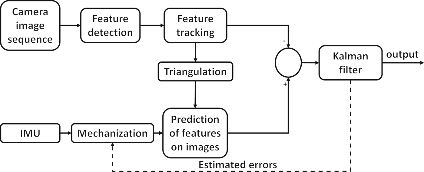
This section discusses the details of the tightly coupled integration of INS/Stereo VO proposed in this work. Before going further, the definition of coordinate frames is illustrated. The world frame for visual odometry is the left camera frame at the first epoch. The IMU body frame is defined as right, forward and up while the local-level frame is defined as east, north and up. Moreover, the camera frame at each epoch refers to the left camera frame. The implementation procedures can be summarised as follows. Based on the estimation of position, velocity and attitude at the previous epoch, the current camera pose can be predicted by the system dynamics model provided by the IMU with Equation (4). The 3D coordinates of features are known by triangulation of stereo cameras at the previous epoch. With known features and predicted camera pose, the predicted image pixel coordinates of features can be achieved by re-projection using Equations (2) and (3). The difference between the predicted and actually measured image pixel coordinates of features is the measurement update in EKF. The procedure is shown in Figure 2.
System architecture.

The state vector in EKF is the error-state explained in Equation (5), given by
 $$x = \left[\matrix{ \delta {r}^l & \delta {V}^l &{\varepsilon}^l &\delta {f}^{\!b} &\delta {\omega}^b } \right]^T$$
where each notation has the same meaning in Equation (7). With the dynamic matrix in Equation (7), the transition matrix can be simplified as
 $$\Phi_{k,k-1} = I + F^{l} dt$$
where I is the identity matrix, dt is the time interval, F l is the dynamics matrix in Equation (7) and k is the current epoch. The equations involved in implementing the EKF are provided below
 $$\eqalign{X_k^- &= \Phi_{k,k-1} X_{k-1}\cr P_k^- &= \Phi_{k,k-1} P_{k-1} \Phi_{k,k-1}^T + GQG^T\cr K_k &= P_k^- H^T \lpar HP_k^- H^T + R\rpar ^{-1}\cr X_k &= X_k^- + K_k \lpar Z_k - HX_{k-1}^- \rpar \cr P_k &= \lpar I - K_k H \rpar P_k^{-}}$$
where Φ k, k−1 is the transmission matrix, which is described in Equation (9), X k − P k − are the a priori state vector and covariance respectively at epoch k, G is the shaping matrix, Q is the driven white noise and H is the design matrix.
The key to implementing the tight integration is to find out the relationship between the pixel coordinate mis-closure and the error-state, namely the design matrix. The derivatives for the design matrix are presented as follows. According to Equations (2) and (3), the coordinates of features in the camera frame need to be predicted in order to re-project the features on the current image plane. However, the 3D coordinates of features are obtained by triangulation in the previous camera frame, which has to be transformed to the current camera frame. As illustrated before, a world frame is set up to uniformly denote the coordinates. Based on the estimated results (e.g. camera position and attitude) of the previous epoch, the feature coordinates can be transformed to the world frame. Then, to transform the feature coordinates to the current camera frame, the current camera position and attitude have to be known, which can be achieved by the mechanisation of the IMU. Finally, we can obtain the feature coordinates in the current camera frame to do the re-projection. Equation (11) below shows the transformation of feature coordinates in the previous camera frame to the world frame, given by
 $$feature^w = R_{l_0}^w R_{l_{k-1}}^{l_0} R_b^{l_{k-1}} R_c^b feature^p + T_{l_0 p}^w$$
where feature
w
are the feature coordinates expressed in the world frame, feature
p
are the feature coordinates in the previous camera frame obtained by triangulation,
 $R_{i}^{j}$
represents the rotation matrix from frame i to frame j, c is the left camera frame, b is the IMU body frame, l
k−1 is the local-level frame at the previous epoch, l
0 represents the local-level frame at the first epoch, w is the world frame namely the left camera frame at the first epoch and
 $T_{l_{0} p}^{w}$
is the translation of the camera from the beginning to the previous epoch expressed in the world frame. The rotation matrices
 $R_{l_{0}}^{w}$
and
 $R_{c}^{b}$
are available by initialisation and lever arm respectively and
 $R_{b}^{l_{k-1}}$
and
 $T_{l_{0} p}^{w}$
are available by the estimation (attitude and position) of the previous epoch. The rotation matrix
 $R_{l_{k-1}}^{l_{0}}$
can be neglected if the translation from the beginning is not too far because of minimal rotation. Otherwise, the rotation can be achieved as
 $$R_{l_{k-1}}^{l_0} = R_{e}^{l_0} R_{l_{k-1}}^{e}$$
where e represents the ECEF (Earth-Centred, Earth-Fixed) frame. The rotation from LLF to ECEF can be given by
 $$R_{l}^{e} = \left[\matrix{ -\sin \lambda &-\sin \varphi \cos \lambda &\cos \varphi \cos \lambda \cr \cos \lambda &-\sin \varphi \sin \lambda &\cos \varphi \sin \lambda \cr 0 &\cos \varphi &\sin \varphi } \right]$$
The obtained feature coordinates in the world frame now have to be transformed to the current camera frame to conduct the re-projection, in order to predict the image pixel coordinates on the current image. The rotation and translation in Equation (2) can be obtained by the mechanisation of the IMU in the current epoch. After updating the position and attitude using Equation (4), the translation from the beginning to current epoch can be denoted in the world frame, given as
 $$T = R_b^c R_{l_0}^b R_e^{l_0} \lpar r^e - r_0^e \rpar$$
where T is the translation expressed in the world frame, r
e
is the current IMU position expressed in the ECEF, while
 $r_{0}^{e}$
is the initial IMU position expressed in the ECEF. The rotation matrices
 $R_{l_{0}}^{b}$
and
 $R_{e}^{l_{0}}$
are available by initialisation,
 $R_{b}^{c}$
is known from the pre-measured lever-arm. With known latitude, longitude and height, the ECEF coordinates can be obtained by
 $$\left[\matrix{ x \cr y \cr z } \right] = \left[\matrix{(R_n + h) \cos \varphi \cos \lambda \cr (R_n + h) \cos \varphi \sin \lambda \cr [R_n (1 - e^2)+ h] \sin \varphi} \right]$$
The rotation from world frame to current camera frame can be written as
 $$R_w^c = R_b^c R_l^b R_{l_0}^l R_w^{1_0}$$
where
 $R_{l}^{b}$
is the rotation matrix from the LLF to IMU body frame, which can be obtained by the updated attitude. The other matrices are the same as before. The rotation and translation in Equation (2) is
 $$R = R_w^c; t = -R_w^c T$$
T is the translation obtained by Equation (14). Therefore, Equation (1) can be rewritten as
 $$X^c = R_w^c X^w = R_b^c R_l^b R_{1_0}^l R_w^{l_0} (feature^w - T)$$
where X c represents the predicted feature coordinates in the current camera frame and X w is the vector from perspective centre to a feature in the world frame. With Equation (3), the features can be re-projected on the image plane to get the predicted pixel coordinates of the feature. When measured feature image pixel coordinates are available, the measurement update in EKF can be formed as
 $$Z_k = \left[\matrix{u & v } \right]_{measured}^T - \left[\matrix{u & v} \right]_{predicted}^T$$
where Z k is the measurement update in the EKF. According to Equations (2) and (3), we can see that the measurements are related to the position and attitude. The design matrix is given by
 $$\eqalign{H &= \left[\matrix{H_r &0_{2 \times 3} & H_{\varepsilon} &0_{2 \times 3} &0_{2 \times 3} } \right] \cr H_r &= {\partial z \over \partial X^c} {\partial X^c \over \partial r^l} \cr H_{\varepsilon} &= {\partial z \over \partial X^c} {\partial X^c \over \partial \varepsilon}}$$
where H
r
and
 $H_{\varepsilon}$
represent the design matrix elements related to position error and attitude error. The partial derivative with respect to X
c
can be obtained easily by Equation (3), given by
 $${\partial z \over \partial X^c} = C = \left[\matrix{{f_x \over z} &0 &{u_0 \over z} - {x \over z^2} \cr 0 &{f_y \over z} &{v_0 \over z} - {y \over z^2} } \right]$$
where x, y, z, f
x
, f
y
, u
0 and v
0 are the same as in Equation (3). From Equation (18), it can be seen that the predicted feature coordinates in camera frame X
c
are related to position error and attitude error. The rotation matrix
 $R_{b}^{c}$
,
 $R_{l}^{l_{0}}$
,
 $R_{w}^{l_{0}}$
in Equation (18) can be treated as constant. The differential equation of Equation (18) can be given as
 $$\delta X^c = -R_b^c \psi R_l^b R_{l_0}^l R_l^{l_0} X^w - R_b^c R_l^b R_{l_0}^l R_w^{l_0} \delta T$$
where ψ represents the skew-symmetric matrix of attitude errors, namely pitch, roll and yaw errors
 $(\delta p, \delta r, \delta y)$
, given by
 $$\psi = \left[\matrix{ 0 &-\delta y &\delta r \cr \delta y &0 &-\delta p \cr -\delta r &\delta p &0 }\right]$$
δ T in Equation (22) is the translation error in the world frame, which can be expressed as
 $$\delta T = -R_b^c R_{l_0}^b R_e^{l_0} \delta r^e = R_b^c R_{l_0}^b R_e^{l_0} M \delta r^l$$
where δ r e is the position error in the ECEF, M denotes the transformation from δ r e to δ r l , which can be derived from Equation (15), namely the relationship between Cartesian coordinates in the ECEF and latitude, longitude and height as
 $$M = \left[\matrix{ -(R_n + h) \sin \varphi \cos \lambda &-(R_n + h) \cos \varphi \sin \lambda &\cos \varphi \cos \lambda\cr -(R_n + h) \sin \varphi \sin \lambda &(R_n + h) \cos \varphi \cos \lambda &\cos \varphi \sin \lambda \cr [ R_n (1 - e^2) + h ] \cos \varphi &0 &\sin \varphi} \right]$$
Based on Equations (22) and (23), the following can be derived
 $$\eqalign{\delta X^c &= -R_b^c \psi R_l^b R_{l_0}^l R_w^{l_0} X^w - R_b^c R_l^b R_{l_0}^l R_w^{l_0} R_b^c R_{l_0}^b R_e^{l_0} M \delta r^{l} \cr &= -{\partial z \over \partial X^c} R_b^c \psi X^b - R_b^c R_l^b R_{l_0}^l R_w^{l_0} R_b^c R_{l_0}^b R_e^{l_0} M \delta r^{l} \cr &= {\partial z \over \partial X^c} \cdot R_b^c \Omega^b \varepsilon - {\partial z \over \partial X^c} R_e^c M \delta r^l}$$
where
 $R_{e}^{c}$
represents the rotation matrix from the ECEF to the current image frame, Ω
b
is the skew-symmetric matrix of feature coordinates in the IMU body frame and ε is the attitude error in the state vector. Combining Equations (21) and (24), the elements in the design matrix with respect to position and attitude error can be obtained:
 $$\eqalign{H_r &= {\partial z \over \partial X^c} {\partial X^c \over \partial r} = -CR_e^c M \cr H_{\varepsilon} &= {\partial z \over \partial X^c} {\partial X^c \over \partial \varepsilon} = CR_b^c \Omega^b}$$
Thus, the derivation of the design matrix for a tight integration of IMU and stereo visual odometry in the LLF has been achieved. Test results are presented in the next section.
4. TESTS AND RESULTS
Karlsruhe Institute of Technology and Toyota Technological Institute (KITTI) datasets are used to test tight integration of the INS/Stereo VO. A Global Positioning System (GPS)/IMU unit and stereo cameras are mounted on the roof of a land vehicle. The lever arms between the IMU and stereo cameras are accurately measured before the field test. The rectified and calibrated stereo images are already synchronised with the IMU datasets. The data sampling rate of both stereo images and inertial datasets are 10 Hz. The GPS/IMU used is OXTS RT 3003, which is a MEMS-based IMU, and the greyscale cameras are Point Grey Flea 2 (FL2-14S3M-C). The GPS/IMU processed results are used as the reference to verify the effectiveness of the proposed method in different scenarios. The accuracy of the reference used is centimetre-level in most cases since differential GPS is applied to remove most errors. In some challenging scenarios where GPS cannot receive enough satellite signals, the reference would suffer accuracy degradation. For the datasets used in this paper, this only happens in a small part in the second dataset, which would not affect the accuracy assessment.
The stereo VO results and the loose integration results are compared with the proposed tightly coupled method. For stereo VO, a Harris corner detector is used to find features on images and a Kanade-Lucas-Tomasi (KLT) feature tracker is applied to track corresponding features between consecutive epochs. In order to avoid too many mismatched features and optimise the distribution of features in the image, bucketing is also applied. In bucketing, the image is divided into nine rectangular parts in which a certain number of features are randomly selected. It is still inevitable to encounter mismatched features or moving objects on images, which have to be removed. In order to filter out the outliers of visual measurements, the RANdom SAmple Consensus (RANSAC) method is used. Specifically, a 200-time iteration, in which a certain number of features are randomly selected each time, is applied in resection to find out the rotation and displacement between two adjacent epochs. The rotation and translation with a maximum number of inliers is chosen as the correct ego-motion and the inliers are kept as the image correspondences at consecutive epochs. The rotation and displacement with respect to the first epoch can be achieved by the accumulation of rotation and translation of two adjacent epochs. Sarvrood and Gao (Reference Sarvrood and Gao2014) and Geiger et al. (Reference Geiger, Ziegler and Stiller2011) have detailed the method of stereo VO. Both stereo VO implementations with and without windowed bundle adjustment are compared with the proposed method. Also of note is that all the detection and tracking methods used by the stereo VO and the tight integration are the same. For the loose integration of IMU and stereo VO, the implementation of the stereo VO adopts the same method illustrated above. The outputs of stereo VO and IMU mechanisation are integrated directly instead of fusing the pixel coordinates in the tightly coupled integration.
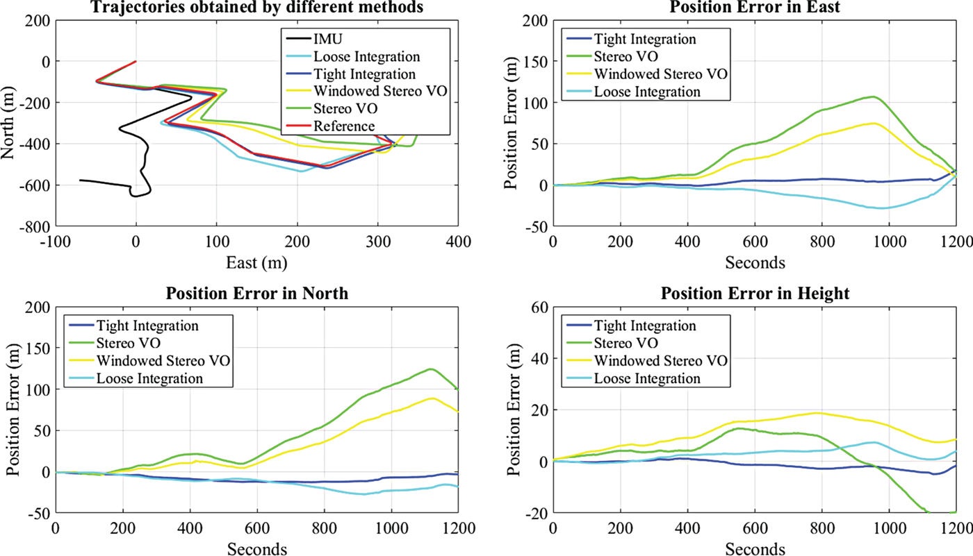
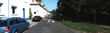
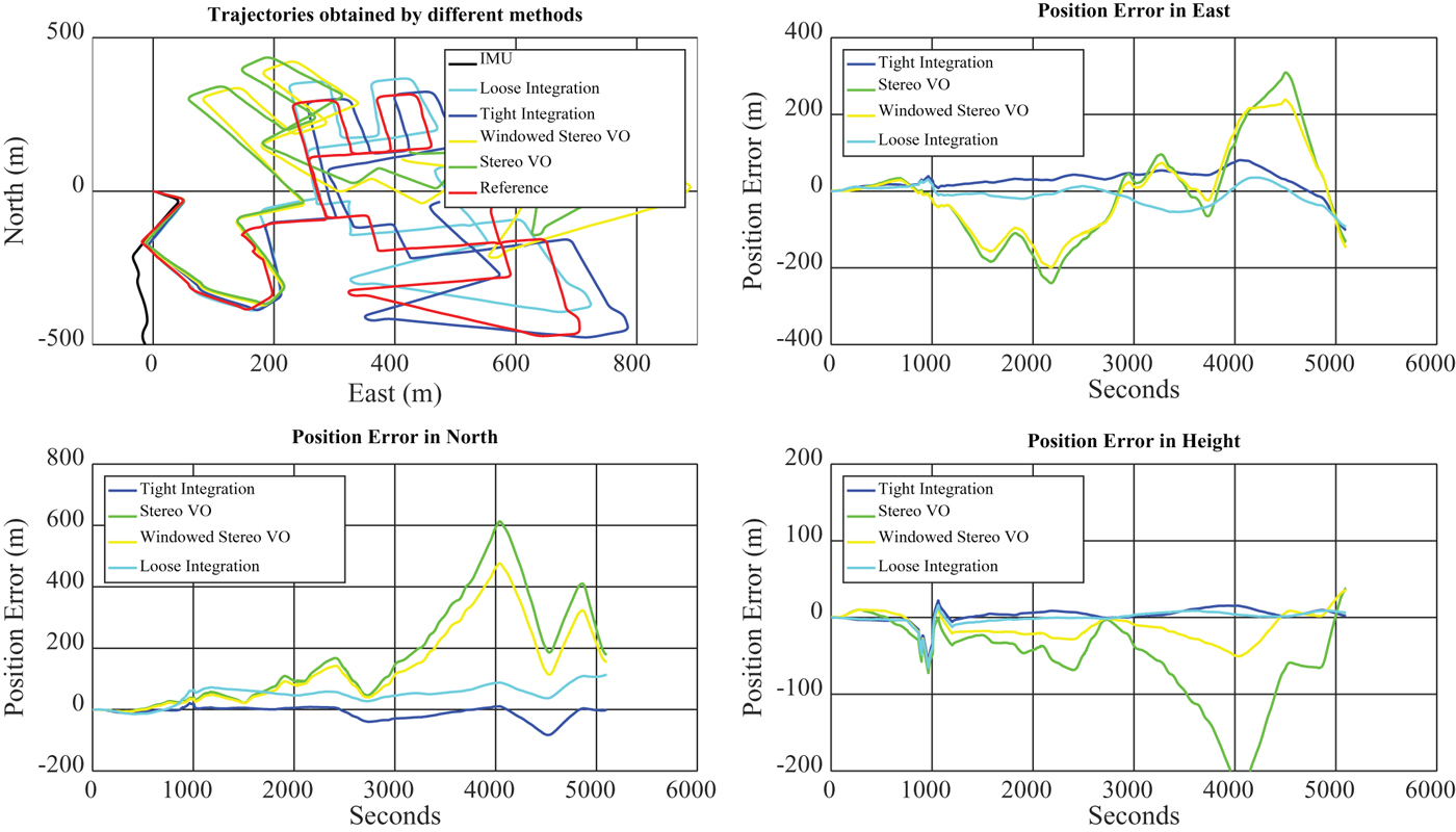
The first dataset contains 1,200 epochs (two minutes), and was collected in a residential area with several manoeuvres in the City of Karlsruhe in Germany (Figure 3). The distance travelled by car for the first dataset is approximately 940 metres. The trajectories obtained by different methods and the position errors in east, north and height are plotted in Figure 4.
First experiment environment.

Trajectories and position errors of each solution for the first dataset.

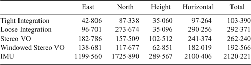
The upper left subplot of Figure 4 shows the trajectories obtained by each solution. All trajectories obtained by the different methods start at (0, 0). The reference solution as well as the solutions from tight integration, loose integration, stereo VO, stereo VO with windowed bundle adjustment and IMU mechanisation are given with different colours. As shown in Figure 4, tight integration outperforms the other methods. The stereo VO adopts the same feature detection and matching strategies as in the integrated solution. However, it can be seen that the result obtained by stereo VO drifts quickly, compared with the integrated solutions. Even with windowed bundle adjustment applied, the stereo VO cannot achieve the same accuracy as the integrated solutions. The loose integration also improves the solution accuracy of the individual sensor, but is still worse than the proposed tight integration method. To see the position accuracy clearly, the position errors of each solution are plotted in the remaining three subplots in Figure 4. The IMU mechanisation result is the worst and its position errors in each direction are not plotted. It is obvious that the tight integration of INS/Stereo VO has the smallest errors in three directions, which is less than 15 metres most of the time. The Root-Mean-Square Error (RMSE) for different solutions is shown in Table 1. From Table 1, it can be seen that the stereo VO and IMU mechanisation results generate large RMSEs while the integration methods largely reduce the drift with the smallest RMSE in every direction. Compared with loose integration, the proposed tight integration is better in every direction and the total RMSE is only half of the loosely coupled integration. This is mainly because the tightly coupled integration takes full advantage of the measurements of each individual sensor.
Position RMSE of each solution for the first dataset (Unit: metre).

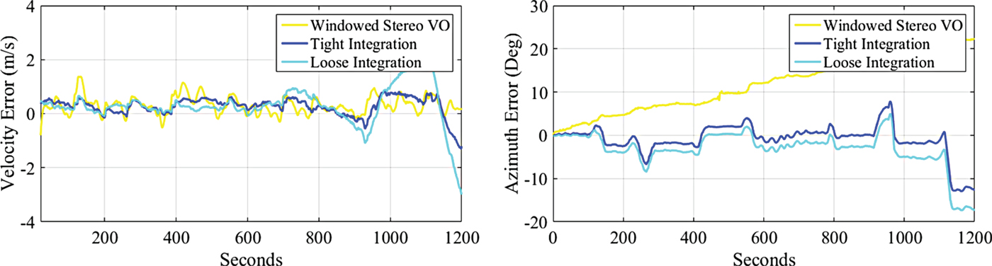
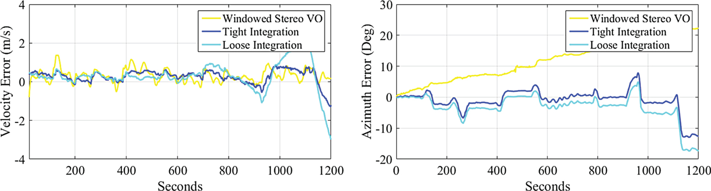
Another advantage of the tightly coupled integration method is that the velocity can be obtained directly instead of using position to calculate the velocity in stereo VO which can generate an unstable output with large noise. Usually, the velocity of the stereo VO has to be processed (filtering out spikes and smoothing) before being used in other applications. The left figure in Figure 5 shows the forward velocity errors obtained directly from the proposed method and the post-processed result of stereo visual odometry. A slight improvement in the forward velocity can be achieved. The RMSE of the forward velocity error obtained by the proposed method is 0.438 m/s while the RMSE of stereo VO with windowed bundle adjustment applied is
 $0{\cdot}449\,\hbox{m/s}$
. The azimuth obtained by the proposed method is much improved, which is shown in the right figure in Figure 5. Compared with the loose integration result, the velocity estimation of the tightly coupled integration is more accurate. The azimuth accuracy of the loose integration is greatly improved compared with the windowed stereo VO, which is less than 10° most of the time. The proposed method outputs more accurate azimuth (RMSE:
 $3{\cdot}68^{\circ}$
), compared with loose integration (RMSE:
 $5{\cdot}20^{\circ}$
). Although the pixel measurements are directly related to the position and attitude, the velocity can be corrected since it is closely coupled with the position and attitude solutions. Therefore, the tight integration improves not only the position results, better velocity and azimuth estimation can be achieved.
Forward velocity errors and azimuth errors of INS/Stereo VO with windowed bundle adjustment for the first dataset.

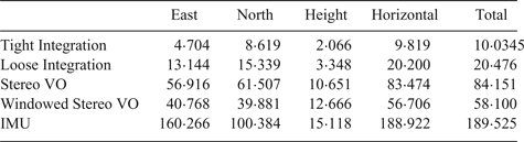
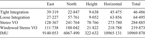
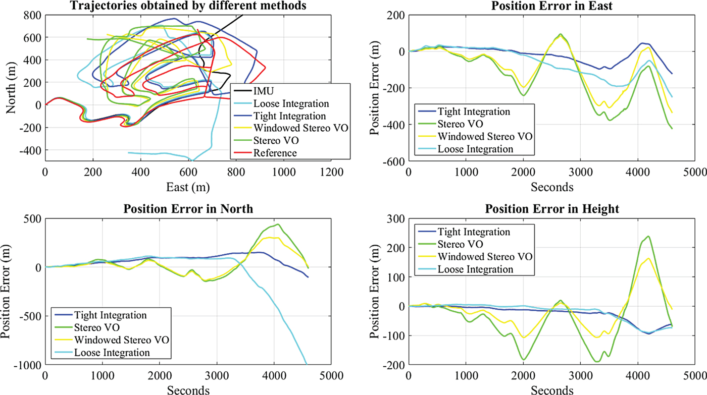
To test the performance of the proposed method over a longer period, a second dataset with 5,100 epochs (8·5 minutes) is applied. Similar to the first dataset, the lever arm is measured before data acquisition and the stereo images are rectified and calibrated. The scenario of the second dataset is similar to the first one, which can be seen from Figure 6. The total distance of the second trajectory is approximately 4,105 metres. The trajectories and position errors of each method are shown in Figure 7. It can be seen that the drift of the proposed method is the smallest one, compared to the other methods. From Table 2, it can be seen that the position accuracy of tightly coupled integration is the best in each direction. The RMSE of the proposed method is only 20% of the stereo VO in the horizontal plane and 71% of the loose integration. Due to a much longer period, the IMU mechanisation errors accumulate up to thousands of metres. The RMSE of the forward velocity estimated by the tight integration is similar to the stereo VO
 $(0{\cdot}74\,\hbox{m/s})$
, which is better than the loose integration
 $(1{\cdot}07\,\hbox{m/s})$
. However, for the azimuth estimation, loose integration outperforms the tight integration. The RMSEs for loose integration and tight integration are
 $6{\cdot}22^{\circ}$
and
 $8{\cdot}61^{\circ}$
respectively.
Second experiment environment.

Trajectories and position errors of each solution for the second dataset.

Forward velocity errors and azimuth errors of INS/Stereo VO with windowed bundle adjustment for the second dataset.

Position RMSE of each solution for the second dataset (Unit: metre).

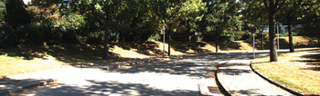
The results from both datasets demonstrate better performance using the proposed algorithm in residential areas. One more dataset collected in a suburban area is also tested. This dataset was collected on a road with trees on both sides, which is shown in Figure 9. The distance of this dataset is about 4,980 metres. The trajectories and position errors are plotted in Figure 10. This time, the position accuracy of the tight integration solution is worse than the results with the previous two datasets. However, the drift is still within half of the stereo VO with bundle adjustment applied in the horizontal plane, which can be seen from the RMSE given in Table 3. The loose integration starts to drift quickly after 3,000 epochs, which makes the overall horizontal RMSE worse than the stereo VO. The performance of the loose integration is not as stable as the proposed tightly coupled integration.
Third experiment environment.

Trajectories and position errors of each solution for the third dataset.

Relative horizontal position error of each method using three datasets.

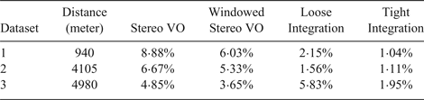
To see the horizontal position accuracy more clearly, the relative horizontal position error for each test is provided in Table 4. It can be seen that the relative horizontal position error for all three datasets using the proposed method is less than 2%, which is much better than the stereo VO.
Relative horizontal position error of each method using three datasets.

5. CONCLUSIONS
The implementation of tightly coupled integration of inertial sensors and stereo cameras is explored in detail. The integration method effectively limits the quick drift of inertial sensors and has a more stable performance than stereo VO and loose integration. The error model is based on the conventional IMU model in the local-level frame. With the system dynamic information provided by the IMU mechanisation and the coordinates of features obtained by triangulation of stereo cameras, the pixel coordinates of features can be predicted by re-projection. The difference between the predicted pixel coordinates and the actually obtained pixel coordinates is applied to correct the system errors. Since the proposed method is based on the most commonly applied inertial error model in the local level frame, one advantage is that the integrated system can be easily augmented with other sensors (e.g. GNSS receiver) by expanding the measurement vector and the state vector to accommodate new measurements.
The datasets collected by a land vehicle confirms the effectiveness of the tightly coupled INS/Stereo VO. The GPS/INS results are used as the reference to calculate the output errors of each method. The results show that not only the position error is reduced by fusing the inertial and visual datasets, but also the velocity and azimuth estimation can be improved as well. The proposed tight integration method outperforms the loose integration in terms of accuracy and stability. Compared to the stereo VO, which cannot provide the velocity directly, the tight integration solution provides velocity of the land vehicle with less noise. Capable of providing velocity and azimuth, the integrated system can be used for other applications (e.g. map matching). Bundle adjustment is not applied in the proposed integration method. Compared with stereo VO without bundle adjustment, the improvement of relative horizontal position error can be more than twice as good. The fact that the position errors could be kept within an acceptable range over a longer period without external absolute positioning information such as GNSS signals is a great benefit for navigation in GNSS-denied environments.
ACKNOWLEDGMENTS
Karlsruhe Institute of Technology (KIT) and Toyota Technological Institute is acknowledged for providing stereo vision and GPS/IMU data for public use on their website. China Scholarship Council (CSC) and the Alberta Doctoral Awards for Chinese Students (ADACS) program are acknowledged for financially supporting the research.