


Introduction
In 1992, the MacSharry reform of the Common Agricultural Policy (CAP) introduced the agri-environmental measures (AEMs) that provide payments to farmers who voluntarily commit to environmental measures related to the preservation of the environment and maintaining the countryside. Since the Agenda 2000 reform of the CAP, the application of agri-environmental programs was made compulsory for Member States within the Rural Development Plans (RDPs).
One of the aims of agri-environmental programs is to provide public goods via measures designed to increase positive externalities through agriculture. The conversion and maintenance of organic production is one of the main AEMs in terms of resources supplied by the European Union (EU; European Commission, 2010). Almost all AEMs contain payments in favor of the introduction or maintenance of organic farming (Sanders et al., Reference Sanders, Stolze and Padel2011). Therefore it is logical to conclude that organic farming support is one of the key strategies aimed at maintaining viable rural areas through the provision of environmental benefits and with quality of life improvements (Silva et al., Reference Silva2014).
During the 2000s, the importance of increasing organic farming support in the agricultural policies became a key strategy in rural development policy in many member countries. Organic farming combines environmental benefits through the reduction of chemical inputs and economic benefits through the diversification of economic activities (Peigné et al., Reference Peigné2015), potentially increasing farmers’ income (Kleemann and Abdulai, Reference Kleemann and Abdulai2013; Boncinelli and Casini, Reference Boncinelli and Casini2014). Organic farming practices’ environmental benefits are numerous, i.e., soil conservation, increased biodiversity as well as reduced soil and aquifer pollution. In addition, consumers are more willing to pay a premium price for food produced less intensively with chemicals, perceived as a healthy and ethical choice (Michaud et al., Reference Michaud, Llerena and Joly2012). The environmental benefits justify the public support. However, the ability to combine it with positive private outcomes has involved the strong engagement of the EU. Public support is indispensable since organic farming entails greater risks than conventional agriculture, and conversion costs from conventional to organic can be an entrance barrier (Gardebroek et al., Reference Gardebroek, Chavez and Lansink2010).
Measure 214-sub-measure A1 (hereafter Measure 214) is the main policy instrument in the EU to incentivize organic farming diffusion (Sanders et al., Reference Sanders, Stolze and Padel2011). Measure 214 provides payments to cover additional costs or income foregone as well as transaction costs (EC Reg. 1257/06). Farmers receive payments for conversion to or maintenance of organic farming in order to compensate them for voluntarily entering into the multi-year prescriptions.
Although Measure 214 is mandatory in the EU, the diffusion and the weight of organic products in total agricultural production today differs substantially among European territories. This is due to differences in climate, soil conditions, farm structures, the institutional environment, market forces and economic policies (Schmidtner et al., Reference Schmidtner2012). The spatial variation of these factors is reflected in a spatial heterogeneity of the diffusion of organic production.
Schmidtner et al. (Reference Schmidtner2012) found evidence of economies of agglomeration in organic farming, which are economies of scale external to the farm (Venables, Reference Venables2009), creating regional agglomerations of organic farms. External economies of scale occur when cost per unit of output depends on the size of the industry in a certain area. The existence of external economies of scale is used to explain the existence of specialized areas (Krugman, Reference Krugman1991).
The factors that produce the spatial agglomeration in organic farming could play a key role in the spatial structure of the rate of farm participation in RDP plans dedicated to fostering organic farming. Indeed, the spatial distribution of the quality (Baumgart-Getz et al., Reference Baumgart-Getz, Prokopy and Floress2012) and the quantity (Wilson and Hart, Reference Wilson and Hart2000) of institutions and extension services entails a non-homogeneous distribution of participation in AESs, including organic farming support. In other words, the areas with a certain rate of farm participation in Measure 214 may be likely to be near other areas with a similar rate of participation.
The role of ‘space’ is relevant for the study of crucial economic and social phenomena. From the so-called first law of economic geography formulated by Tobler (Reference Tobler1970, p. 236), which states, ‘Everything is related to everything else, but near things are more related than distant things’, numerous statistical econometrics models (see Fischer and Getis, Reference Fischer and Getis2009) have been proposed to analyze the spatial effects of economic and social events. These quantitative tools test the influence of social norms, the effects of production externalities, the localization pattern and the behavior of social groups (Ward and Gleditsch, Reference Ward and Gleditsch2008; LeSage and Pace, Reference LeSage and Pace2009). In general, a set of similar social norms could be shared within a social group and become relevant for collective behaviors. However, as noted by Alló et al. (Reference Alló, Loureiro and Iglesias2015), the influences of the social groups can have different patterns, and in the case of agri-environment schemes their influence can be greater than that of the social norms.
An investigation into the spatial interactions between agents provides an interpretation of collective behaviors, Marshallian externalities, agglomeration economies and the spillover of local economies. Including spatial interactions in the economic analysis, helps to relax the classical hypothesis of the atomistic agent who makes decisions irrespective of the effects of decisions taken by other agents.
This paper aims to investigate the spatial distribution of farms’ participation in Measure 214. Spatial indicators and a spatial econometrics model are deployed in order to identify the influence of common factors and agglomeration effects on the distribution of participation in organic farms, using Tuscany (central Italy) as our case study.
Tuscany can be considered a suitable case study for several reasons. In Italy, the policies developed by the Rural Development Program under the FEADER fund for the period 2007–2013 are implemented in Italy at regional level, that is, the NUTS 2 Eurostat classification to which Tuscany belongs. In addition, Tuscany shows a very high variability of geographical, climatic and altitude conditions, which determine strong heterogeneity in product specializations. Tuscany also shows relevant differences in socio-economic conditions among its areas. The combination of socio-economic and territorial factors results in a considerable and variegated set of farming systems (i.e., from extensive commodity production to high-value cultivation such as wine grapes and plant nurseries). Altogether, these factors may determine different propensities to enroll in organic measures among the regions and areas. Finally, the high variability of all these factors means the results are less strongly linked to specific situations and facilitates the generalization of the conclusions.
To investigate the spatial effects is crucial for a better understanding of the causes and patterns that determine the spatial concentration of organic farm support. In turn, this is useful for improving the design of policies. As noted by Wollni and Andersson (Reference Wollni and Andersson2014), studying the spatial pattern of the observed outcomes is crucial for policy planners, because it separates the individual determinants from the contextual determinants of farms’ participation in rural development measures. Indeed, whether the influence of neighborhood networks exists and to overcome the entrance barriers to adopting organic production, the policy can be developed at community level. All these results help to identify potential criteria to improve the design of better policies to foster the diffusion of organic farming and promote less intensive agriculture.
This paper is organized as follows: the section ‘Literature review’ reviews the literature. The sections ‘Empirical strategies’ and ‘Empirical results’ present the estimation method and the empirical findings on the spatial association of participation rates in Measure 214 in Tuscany. The section ‘Conclusion’ concludes the paper.
Literature review
The determinants of organic adoption have been extensively investigated in the agricultural economics literature. Several authors (such as Läpple and Van Rensburg, Reference Läpple and Van Rensburg2011; Mzoughi, Reference Mzoughi2011; Läpple, Reference Läpple2013; Läpple and Kelley, Reference Läpple and Kelley2013) have highlighted how organic farming is more likely to be found in larger farms, located closer to urban areas, and carried out by younger and more educated farmers, concerned about environmental issues.
In addition, contextual factors for going organic can be determined. The list includes the influence of local institutions (Genius et al., Reference Genius, Pantzios and Tzouvelekas2006; Morone et al., Reference Morone, Sisto and Taylor2006; Padel et al., Reference Padel, Roecklinsberg and Schmid2009; Blanc and Kledal, Reference Blanc and Kledal2012) and the geographical framework in which farmers operate (Kostandini et al., Reference Kostandini, Mykerezi and Tanellari2011).
However, few studies have focused on the role of neighborhood effects in organic production. The hypothesis that the location and distances are central factors for economic activities and market structure is consistently recognized by economic theory, in particular economic geography and regional economy, which have formalized concepts such as spatial interactions, diffusion processes and hierarchies of places. Schmidtner et al. (Reference Schmidtner2012) stressed that agriculture, which is strongly linked to land as the main production factor, should seem less influenced by the agglomeration effects emphasized by the new economic geography (Krugman, Reference Krugman1991; Fujita et al., Reference Fujita, Krugman and Venables2001), yet organic farming seems to show agglomeration patterns due to external factors (Yang et al., Reference Yang2014).
Whether or not organic farming is seen as an innovation, a spatial structure in organic agriculture can be produced by the diffusion model of innovation in the primary sector. Rogers (Reference Rogers1995) demonstrated that the diffusion of innovation in the agriculture process is performed by innovative farmers, and is then transmitted to others by an imitation process or through networks (peers to peers; mass media; or extension service networks). In the case of participation in RDP measures, neighborhood networks, uneven distribution of extensions in service quality and policy design parameters may determine a spatial agglomeration. The neighborhood networks produce effects through imitation and may then cause agglomeration by imitation (Case, Reference Case1992; Bandiera and Rasul, Reference Bandiera and Rasul2006; Conley and Udry, Reference Conley and Udry2010) and peer experience (Hübler et al., Reference Hübler2012; Goulet, Reference Goulet2013). The quality of extension services may cause high cost of information, influencing transaction costs for participation (Mettepenningen et al., Reference Mettepenningen, Verspecht and Van Huylenbroeck2009) and policy parameters such as targeting and priorities may determine the higher probability of receiving payments or higher payment levels, in turn offering higher profitability (Raggi et al., Reference Raggi2015).
Doring and Schnellenbach (Reference Doring and Schnellenbach2006) demonstrated the existence of a direct relationship between innovation spillovers and local economies. A spatial spillover is a situation in which the dynamics in a certain area directly or indirectly influence the pattern of neighboring local economies. In practice, if the diffusion of innovation is geographically determined, it is possible to find a spatial relationship in the levels of agricultural value-added. Again, Doring and Schnellenbach (Reference Doring and Schnellenbach2006) stress that the spillover effects of innovation and knowledge can explain the formation of geographical clusters where there are areas with the same economic structure, sectorial specialization, income levels and growth patterns, as well as similar and complementary technologies.
The previous studies highlight the spatial clustering of organic farming (Parker and Munroe, Reference Parker and Munroe2007; Schmidtner et al., Reference Schmidtner2012) where regions with high proportions of organic farming tend to be close to other regions with high shares of organically farmed land. Others (Lewis et al., Reference Lewis, Barham and Robinson2011; Läpple and Kelley, Reference Läpple and Kelley2015; Alló et al., Reference Alló, Loureiro and Iglesias2015) have reported that there is a spatial agglomeration even at the individual level, i.e., farmers are likely to adopt organic production if their neighborhoods adopt organic production. Wollni and Andersson (Reference Wollni and Andersson2014) and Läpple and Kelley (Reference Läpple and Kelley2015) found that social conformity is the main factor in spatial clustering, i.e., the tendency of the individual to behave in compliance with the individual's social group. In general, the previous studies stress how external economies of scale, norms, neighborhood networks and communities play a key role in the decision of farmers to adopt or maintain organic farms.
However, the spatial effects of rural development policy have not been sufficiently investigated. Bartolini et al. (Reference Bartolini, Raggi and Viaggi2012) and Yang et al. (Reference Yang2014) investigated the spatial regime (association or heterogeneity) of participation in Measure 121 in Emilia-Romagna (Italy) and the habitat management, bird conservation and water habitats in Scotland (UK). They underline the importance of spatial analysis in improving the predictability of participation in rural development measures, taking into account agglomeration effects and spatial dependencies.
The present paper aims to combine the analysis of the spatial pattern of the adoption of organic farming with the rate of participation in Measure 214. The underlying hypothesis is that the same factors that affect the agglomeration of organically farmed land play a key role in a farmer's decision to participate in Measure 214. This hypothesis is studied with the calculation of spatial statistics and is assessed by applying an econometric model that, by explicitly incorporating the spatial structure of participation in Measure 214, returns a more robust analysis of determinants.
Empirical strategies
A growing body of literature deals with understanding the spatial pattern of economics and social phenomena. A flourishing literature in the field of agricultural economics has applied spatial analysis to improve the model's ability to understand innovation diffusion, policy impacts and land use changes (Bell and Dalton, Reference Bell and Dalton2007; Brady and Irwin, Reference Brady and Irwin2011). Several studies include space and location as a proxy for the difference in demand for environmental services (see, e.g., van Leeuwen and Dekkers, Reference van Leeuwen and Dekkers2013) or for participation costs, while only a few papers have refined the estimation to include the effects of spatial spillover (see Schmidtner et al., Reference Schmidtner2012).
Methodology
The spatial agglomeration of participation rates in Tuscany was analyzed in two steps. First, the spatial correlation of the participation rate in support for organic farming was estimated using Moran's I index, which is used to test spatial correlation against the null hypothesis of no spatial correlation. It was calculated as:
 $$\qquad I = \displaystyle{n \over {\sum\nolimits_{i = 1}^n {w_{ij}}}} \cdot {\textstyle{{\sum\nolimits_{i = 1}^n {\sum\nolimits_{\,j = 1}^n {(x_i - \bar x)(x_i - \bar x)w_{ij}}}} \over {\sum\nolimits_{i = 1}^n {(x_i - \bar x)^2}}}}, $$
where w ij is the spatial weight obtained by a spatial function between area i and j; and x i and x j are the outcomes in the area i and j, respectively. For each geographical unit a weight w ij = 1 is assigned if the geographical units i and j are spatially contiguous; w ij = 0 otherwise. The definition of contiguity is that two geographical units share a part of their border. The spatial statistics are performed in order to test whether the observations are spatially dependent.
Moran's I indicator is the global measure of spatial autocorrelation which provides an indication of the spatial pattern of the phenomena. The global measure helps to understand the overall spatial nature of the distribution of the participation rate by summarizing different spatial relationships in the data.
However, the global indicators do not contain information for a particular local spatial unit. Therefore, Anselin (Reference Anselin1995) proposed the Local Indicator of Spatial Association (LISA), which identifies more effective observations and spatial clustering by decomposing Moran's I to identify and test the regions that most contribute to Global Moran's I. The Local Moran statistic also identifies a specific location of the spatial clustering.
In order to estimate the spatial dependence and control participation factors, a spatial econometric model is applied. The spatial econometric modeling can incorporate the spatial structure in regression models detected by the spatial correlation statistics.
The model specification for spatial econometrics relates to the identification of the casual effects between space and economic factors and the selection of the relation among spatial units. The spatial econometrics literature identifies three main models to simulate the causality of space in explaining economic factors: spatial lag models, spatial error modes and spatial Durbin model. The spatial lag and spatial error models assume that the dependent variable is the one affected by the space, while in the spatial Durbin model it affects one or more of the independent variables (Mur, Reference Mur2013). The spatial lag corrects effects, assuming a spatial relation within the dependent variable; meanwhile, the spatial error coefficient corrects heteroscedasticity due to spatial dependence in the error term and unobserved variables. Interactions among spatial units are generally hypothesized as derived by neighborhood or by distance, whereby the strength and direction of interactions between spatial units is captured by a spatial weighting matrix. Hence in the first approach, weight matrices are assumed to be those spatial units that share part of the border, while in the second approach spatial units are interrelated based on distance or on diffusion function (see Mur, Reference Mur2013). The paper's research goal is to investigate the direct influence of participation rate in contiguous areas; therefore, a spatial lag model using a first-order contiguity matrix is applied.
This model was been chosen on the basis of several considerations. The models mentioned previously are not nested, and thus it is difficult to discriminate among the models purely on statistical grounds (Ward and Gleditsch, Reference Ward and Gleditsch2008). Therefore, the selection of the model is made relative to the goals of the paper's research questions. Since it seems very plausible that the spatial relation is due to direct effects rather than a systematic non-observed component that induces spatial correlation in the errors of the model, the spatial error model is not appropriate for testing the paper's hypothesis. This is also the case for the Durbin model, because the focus of the investigation is the endogenous area factors that induce farms to participate in Measure 214.
Following Anselin (Reference Anselin1988, Reference Anselin and Baltagi2001) and LeSage and Pace (Reference LeSage and Pace2009), the spatial lag model has the following form:
 $$\qquad \eqalign{& y\, =\, \rho {\rm \bf W}y \,+ \,{\rm \bf X}\beta\,+\,{\rm \varepsilon} \cr & {\rm \varepsilon}\,\sim\,N(0,\sigma ^2 {\rm \bf I}_{\rm \bf n} );} $$
where y and X are the dependent variable and the matrix of independent variables, respectively; ρ is the coefficient of spatial association; W is the matrix of spatial weight built as a function of the contiguity of municipalities (i.e., local geographical administrative areas); ε is the error term with spherical disturbance distributed normally; and I n is an identity matrix. The term W y is called the spatial lag. The application of (2) implies the fundamental hypothesis that the realization of y in the ith region is determined/conditioned by the realization in the contiguity region of j, while ρ measures the intensity of this connection. Moreover, the spatial lag model is designed to detect evidence of neighborhood effects and, again, ρ measures the intensity of this effect (Ward and Gleditsch, Reference Ward and Gleditsch2008). As mentioned in the model specification, the spatial effects are estimated taking into account neighborhood influence among municipalities. Hence, matrix W is a symmetric matrix with zeroes on the main diagonal and cells that contain zeroes when two spatial units are non-contiguous, while their value is one at the opposite point. The parameters ρ and β are estimated by maximizing the log likelihood function that contains the contiguity matrix W and the parameter ρ:
 $$\eqalign{{\rm Ln}\,L(\beta, \sigma ^2, \rho )\, =\, &\ {\rm ln} \vert {\rm \bf I} - \rho {\rm \bf W} \vert - N/2{\rm ln}\,(2\pi ) - N/2{\rm ln} (2\sigma ^2 ) \cr & - {\rm} (y - \rho {\rm \bf W} - {\rm \bf X}\beta )^{\prime}{\rm} (y - \rho {\rm \bf W} - {\rm \bf X}\beta )/2\sigma ^2.} $$
On the assumption that the essential determinants to participate in Measure 214 are sustained at an aggregated level, the empirical model estimates the share of participants in this measure at the municipality level. Therefore, the unit of analysis is the municipality, which is the LAU 2 in Italy according to Eurostat territorial units’ classification. The use of the municipality level is for several reasons. As noted by Getis (Reference Getis2009), the spatial structure must be exogenous to the models and must be based on preconceived spatial structures such as administrative boundaries; otherwise, results will be biased. In addition, measurement at local level allows one to consider factors exogenous to the models’ unobserved variables such as farm soil condition, and farmers’ risk behavior.
Data
The variables on the structural features of municipalities are calculated using the data from the sixth Italian agricultural census (2010). Information on the RDP comes from the administrative data of the ARTEA (Regional Rural Payments Agency).
The covariates are classified into four categories. The first category is related to the territorial characteristics. A first variable is related to the share of Nature 2000 areas within each municipality. Then, the classification of the areas is described with dummy variables to check for an altitude effect. Finally, a factor variable is added using the municipalities’ classification in terms of RDP design. The area of the region was classified into five categories, based on inhabitants’ density and the share of agricultural labor in the total labor. Location variables are crucial in the model's geographical rendering of the region, managing different demands on the environmental services. Moreover, locations in different geographical areas may encounter different opportunity costs when shifting productions towards organic farming due to the availability of alternative crop mixes or differences in climate and soil characteristics (Espinosa-Goded et al., Reference Espinosa-Goded, Barreiro-Hurlé and Dupraz2013).
The second group concerns the farmers’ characteristics: the share of farms with male owners, farmers aged below 40, farmers with an agricultural background or a degree and the proportion of part-time farmers. These variables are widely used by the agricultural economics literature to model farmers’ behavior in terms of innovation and farmers’ attitudes towards environmentally friendly practices (Läpple and Van Rensburg, Reference Läpple and Van Rensburg2011). Several authors show that young and highly educated farmers are more likely to participate in agri-environmental schemes due to the low transaction costs to apply the measure (Falconer, Reference Falconer2000).
The third category of variables describes farm structures: the number of cooperatives, the share of individual farms, the share of farms with a potential successor, farms that use only household labor, average Utilised Agricultural Area (UAA) of farms, ratio of UAA and total land and average number of plots in each municipality. Inclusion of those variables in covariates may be done for different reasons. First, a fixed cost of participation may reduce the likelihood of observing participation among small farms (Ducos et al., Reference Ducos, Dupraz and Bonnieux2009), while the plots’ fragmentation increases operative costs and may have positive effects in explaining participation (Bartolini and Brunori, Reference Bartolini and Brunori2014). The involvement in cooperatives or networking may produce differences in the quality of information held by farmers and may reduce the transactions costs (Defrancesco et al., Reference Defrancesco2008).
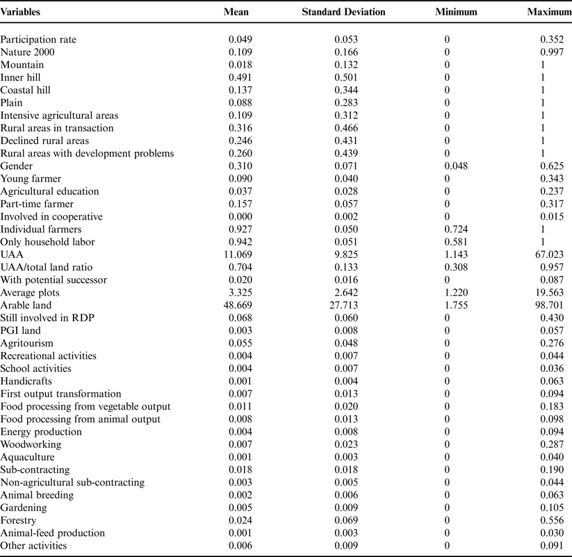
The fourth category is related to the farming system: the number of farms with arable crops, the number of farms with RDP support (other than 214) and with Protected Designation of Origin (PDO) production, and the number of farms involved in other activities such as agritourism, recreational activities, school activities, handicrafts, food processing, energy production, woodworking, aquaculture, agricultural and non-agricultural services, animal breeding, gardening, forestry and animal-feed production, and other activities. This category of variables is included since almost all the papers previously cited included in their analysis variables related to farm systems. In addition, including these variables in the model is relevant for two reasons: a theoretical and a statistical reason. First, inserting these variables in the model makes it possible to detect whether a particular specialization increases the probability of participating in Measure 21. In addition, the variables in other categories are correlated with the variables relating to farm systems. Therefore, endogeneity concerns could arise in the case farm systems variables would be excluded. Table 1 shows the descriptive statistics for all the covariates.
Descriptive statistics.

Empirical results
A total of 5% of farmers in Tuscany participated in Measure 214. The land under Measure 214 accounted for over 10% of the total regional UAA. Figure 1 shows the distribution of the share of beneficiaries across the municipalities in Tuscany.
Spatial distribution of the share of farms participating in organic farming.

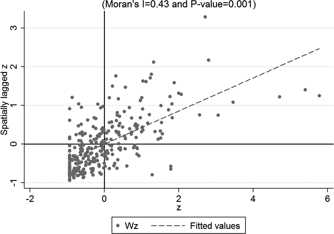
The municipalities of central Tuscany and the northeast had higher participation rates. Lower rates of beneficiaries were found in the northwest. The municipalities with a similar level of participation tended to be grouped in the same areas. The spatial distribution shown in Figure 1 seems to highlight various spatial patterns underlying participation in Measure 214, thus providing evidence of spatial dependence. However, to establish a relation between participation and location, it is necessary to measure the spatial correlation. Figure 2 presents the Moran scatter plot, which provides a graphical interpretation of the spatial association among municipalities.
Moran scatter plot for the share of farm participation in organic farming.

Global Moran's I of 0.43 indicates a positive, significant and relatively high spatial correlation. The significance is tested against the null hypothesis of no spatial correlation, that is to say the randomness of the cases. Therefore, Global Moran's I indicates a stronger geographical clustering; that is, the values of the participation rate in Measure 214 for neighboring municipalities are similar to one another. The z is the standardized variable and Wz is the geographically weighted standardized variable. The slope of the fitted line is equal to Moran's I. In the first quadrant, the points represent the municipalities with high participation rates that are contiguous to other municipalities with high rates. The third quadrant shows municipalities with low participation rates together with neighboring municipalities with low rates. Spatial outliers are in the third and fourth quadrants, i.e., neighboring municipalities with different participation rates.
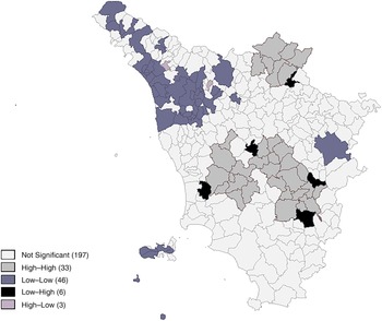
For each municipality the Local Moran is computed and tested for significance by randomization. Figure 3 shows the distribution of Local Moran's I values for each municipality in Tuscany (Local Indicator of Spatial Association, LISA).
LISA of participation rates in organic farming.

The hot and cold spots have the highest values indicating the areas with the strongest association pattern. These municipalities, therefore, are the main ‘contributors’ to the positive and significant global measure of spatial autocorrelation with the rate of participation in Measure 214.
Significant local clusters and spatial outliers are shown in grayscale. The municipalities with the darker color show the ‘hot spots’ or ‘cold spots’, which highlight the spatial clusters. In the hot spots (high–high) the positive spatial association arises from each unit and neighboring units with high participation rates. In the cold spots (low–low) the positive spatial autocorrelation emerges from each unit and the neighboring low values of the variable. The hot spots of participation are located in central and northeast areas, cold spots in the northwest. In addition, Figure 3 highlights that the hot and cold spots in Tuscany are particularly concentrated in geographically distinct areas. This result suggests evidence of the location pattern of participation rates in Measure 214.
The areas with negative Local Moran coefficients originating from significant high and low surrounding values, and areas with negative Local Moran coefficients resulting from low and high surrounding values are sources of spatial non-stationarity. A noteworthy point in Figure 3 is that negative values are only found on a small part of the total area of Tuscany. One may conclude that participation in Measure 214 exhibits elements of strong spatial concentration.
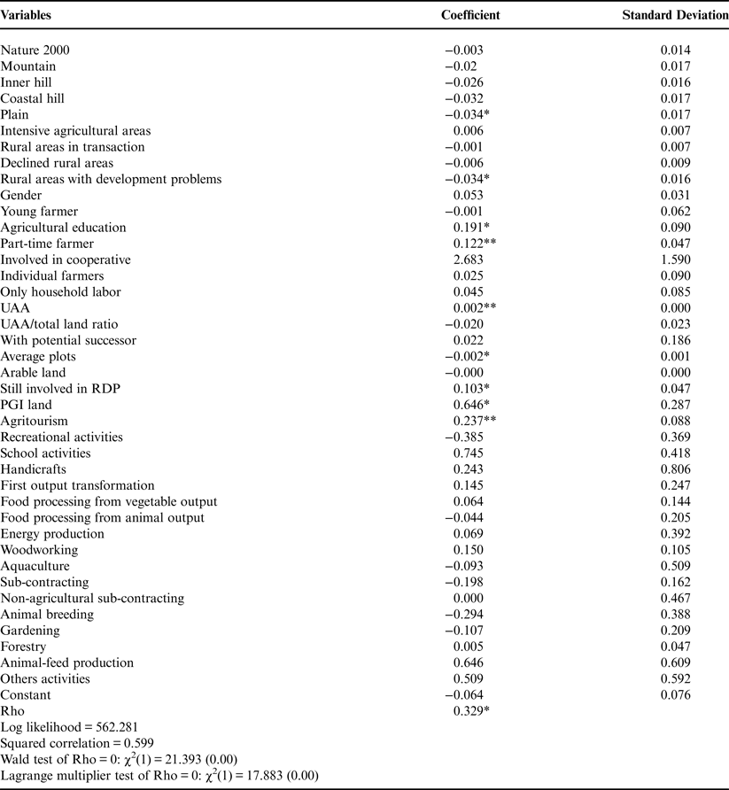
Table 2 shows results of the spatial lag model. The spatial autoregressive coefficient (Rho) has an important influence on the distribution of the farms that apply for funding through Measure 214, thus suggesting the existence of agglomeration effects between areas. If, all other things being equal, the share of participants in a municipality increases by 1%, then the estimated share of participants in the neighboring municipalities increases by 0.329%.
Results of spatial lag model.

Note: *P < 0.05, **P < 0.01.
With regard to the other significant variables included in the model, we can note that the zoning used to design the RDP plan and altitude are significant, but with a weak effect on participation. The location in plain and marginal areas negatively affects the rate of participation in organic farming. Therefore, extreme operating contexts (the best and the worst) have the same effects in predicting the participation rate in Measure 214. The lower participation rate in plain areas could be due by the higher opportunity costs for converting to organic (Alló et al., Reference Alló, Loureiro and Iglesias2015) and thus participating in Measure 214. However, the same hypothesis does not hold in the case of the marginal areas where the opportunity costs are substantially lower than in the plain areas. Thus lower likelihood of participation in Measure 214 seems to be related to the predominance of the transaction costs, since Khaledi et al. (Reference Khaledi2010) stressed that the lack of infrastructures and services increases these kinds of cost and discourages participation in organic farming.
The farm typology within the municipality does not affect the rate of participation, since the only significant variables are the education rate of farmers and the proportion of full-time farmers. Areas with highly educated and full-time farmers are most likely to participate in Measure 214. The results confirm previous literature findings on the role of education in reducing transaction costs associated with the measure's application. Moreover, other social studies have found that well-educated farmers show a strong pro-environmental orientation (Henning et al., Reference Henning, Zhong and Cardona2004). In addition, large farms and those involved in farm holidays or PDO production are also more likely to participate in organic measures. This result seems to indicate that zones oriented to traditional production have some positive interaction factors with organic production. Probably the compliance with PDO rules is in many cases similar to organic standard. This can induce farmers to participate in organic farming measures due to the lower costs of compliance with organic production methods. These results confirm the existence of second-order effects of diversification activity on the creation of areas with higher environment quality (Bartolini and Brunori, Reference Bartolini and Brunori2014).
Finally, a positive factor is the number of farmers who are already participating in other RDP measures. This may be explained by the cost involved in obtaining information or the transaction costs of participating in RDP measures as suggested by Rørstad et al. (Reference Rørstad, Vatn and Kvakkestad2007).
Conclusions
This paper aimed to investigate the determinants of participation rates in Measure 214 taking into account spatial patterns. The results highlight an important spatial dependence in the participation rate highlighted by the significant and positive Rho coefficient in the spatial lag model. This implies that neighborhood effects exist. In addition, if the results of LISA are considered, it is possible to conclude that the spatial association is evident. Hence, the application of a spatial econometrics model is a viable tool to detect the diffusion of agri-environmental schemes.
The results confirm the literature regarding the spatial dependency of participation in AEMs (Yang et al., Reference Yang2014). The latter study found that spatial agglomeration can depend on heterogeneity in agricultural systems due to the effects of climate regimes, and on the farms’ specializations. It can also depend on the different quality of support for RDP applications and the networking of farmers regarding the related regulations.
The areas with a high share of farms that receive support for organic farming are more likely to have neighboring municipalities with high rates. By contrast, areas with low public support are likely to be close to areas with low rates of farms receiving support.
The results of the econometric analysis are similar to the findings of Bartolini et al. (Reference Bartolini, Raggi and Viaggi2012) for Measure 121. Therefore, we make generalizations stressing that the RDP participants are not randomly distributed, but are spatially clustered. The general economic literature calls the specialized areas ‘districts’, and studies their distinctive features. However, this definition does not seem correct in agriculture, where it is better to refer to a cluster. Indeed, the determinants that play a role in the formation of a district are more related to endogenous factors. On the other hand, in agriculture the determinants for the creation of clusters are exogenous factors. This matter is demonstrated based on the model results where none of the farm system variables are significant. Thus, any particular specialization influences the spatial pattern of participation in Measure 214.
The factors that explain spatial participation patterns are the same as those that have been previously discussed in the literature (Schmidtner et al., Reference Schmidtner2012; Alló et al., Reference Alló, Loureiro and Iglesias2015; Läpple and Kelley, Reference Läpple and Kelley2015). However, the main underlying determinants seem to be the information spillovers and economies of scale economies external to the farm which enable farmers to reduce the information and transaction costs of participating in RDPs measures. Less important is the social conformity discussed by several authors (Alló et al., Reference Alló, Loureiro and Iglesias2015; Läpple and Kelley, Reference Läpple and Kelley2015); on the other hand imitation may play a role (Renting et al., Reference Renting, Marsden and Banks2003) as well as knowledge shared by peers (Goulet, Reference Goulet2013).
These conclusions are drawn because the economic literature tries to explain the spatial relations between areas as main factors of the agglomeration effects: information spillover, the external economies of scale, imitation processes and the social conformity. Since none of the previous studies have detected the existence of social norms that drive the willingness to participate in AEMs, a logical deduction is that the main factors that partake in the agglomeration effect are the external economies and the information spillover.
The key role of the neighborhood networks in reducing information and transaction costs for the farmers’ participation suggests that extension services aimed at specific areas may be effective as individually addressed services, as noted by Wollni and Andersson (Reference Wollni and Andersson2014). The results show that policy participation in other measures affects the participation rate in Measure 214 and demonstrate the existence of transaction costs and entrance barriers to participating in RDP measures. Therefore, policy makers need to design eligibility criteria in order to minimize these kinds of costs. If they do not, they will jeopardize the diffusion of organic farming and limit the environmental benefits of this method of production.
The policy implications of the findings are important. The benefits of organic farming, especially the environmental benefits, are localized. Whether or not the policy makers’ goals include the diffusion of organic farming, the existence of significant cold spots and hot spots reveals the existence of areas where participation in Measure 212 is less than ideal. Theoretically, the spatial diffusion of participation should be as homogenous as possible. The policy maker should improve the geographical targeting and design policy tools to eliminate the territorial constraints on participation in RDP measures. In particular, the territorial impact of the role of social groups, the quality of the extension service and the information and transaction costs should receive particular attention during the policy design otherwise the public resources could exacerbate the territorial disparity.
Finally, it must be pointed out that the literature has stressed the importance of the food value chain as a determinant of farms’ behavior (Renting et al., Reference Renting, Marsden and Banks2003). However, this dimension could not be included in the empirical model of the present paper. This is due to several issues. The paper studies the determinants of participation in a policy designed to foster farmers’ maintenance of or engagement in organic farming. The farmers that sell certified organic foods are just a part, even if an important one, of the organic producers. The decision to participate in this measure can be made independent of the influence of the food chain. In other words, organic farming does not necessarily imply organic certification, and thus organic sales. The farmer can be motivated to participate due to personal environmental concerns (Mzoughi, Reference Mzoughi2011); unfortunately these are unobservable. Moreover, a farmer might base the decision to participate purely on cost-benefit considerations, i.e., the farmer expected that the received funds would be greater than the costs of complying with organic regulations, but not enough to cover the cost of organic sale.
One aspect that has not been sufficiently addressed, due to the lack of data, is the analysis of individual farms and farmers’ characteristics and attitudes to participation in Measure 214. The use of secondary data at the LAU 2 level with mean values for each municipality does not take into account the heterogeneity of farms present in the locality.
Acknowledgements
An earlier version of this paper was presented during the XXV ESRS Congress “Rural resilience and vulnerability: the rural as locus of solidarity and conflict in times of crisis” in Florence, Italy 2013 July 29 – August 1. The authors wish to thank the anonymous referees and the Associated Editor for their useful suggestions and comments on an earlier version of the paper.